The essential synergy of MD simulation and NMR in understanding amorphous drug forms

Abstract

Molecular dynamics (MD) simulations and chemical shifts from machine learning are used to predict ¹⁵N, ¹³C and ¹H chemical shifts for the amorphous form of the drug irbesartan. The local environments are observed to be highly dynamic well below the glass transition, and averaging over the dynamics is essential to understanding the observed NMR shifts. Predicted linewidths are about 2 ppm narrower than observed experimentally, which is hypothesised to largely result from susceptibility effects. Previously observed differences in the ¹³C shifts associated with the two tetrazole tautomers can be rationalised in terms of differing conformational dynamics associated with the presence of an intramolecular interaction in one tautomer. ¹H shifts associated with hydrogen bonding can also be rationalised in terms of differing average frequencies of transient hydrogen bonding interactions.

---

1 Introduction

Poorly water soluble drugs are increasingly encountered in drug development pipelines, especially amongst so-called “beyond rule of 5” molecules that do not fit the classical rules for well-behaved small molecule drugs.^1,2 The use of amorphous forms, either by explicit amorphisation of otherwise crystalline phases, or because the molecules are difficult to crystallise, provides a potential solution, since amorphous materials have intrinsically higher solubility than their crystalline counterparts.^3–6

The lack of long-range ordering in amorphous materials creates significant challenges for their characterisation, since diffraction-based techniques are of limited value; the absence of long-range ordering means that there are no Bragg diffraction peaks. Total scattering methods can provide overall pair distribution functions for amorphous materials, but these are of limited value for structural determination since the short-range behaviour is dominated by the immediate bonding environments, and long-range information is missing due to the lack of order.⁷ In contrast, the site-specific nature of NMR allows the local chemical environment around individual sites to be probed. Even if the overall spectra cannot be directly linked to structure, individual spectral features can often be interpreted in terms of local structure and dynamics. In recent work on amorphous forms of the sartan drugs valsartan and irbesartan, for example, we have shown how NMR can be used to connect specific molecular conformers of valsartan to its lack of crystallinity,⁸ and how NMR relaxation reveals distinct molecular dynamics in different parts of the irbesartan molecule that can be linked to the glass transition.⁹ In contrast, however, to current trends in “NMR crystallography” of molecular solids,^10,11 such work relies on largely qualitative interpretations of the NMR data, since it is not feasible to calculate chemical shifts etc. in amorphous materials using first principles methods.

A more subtle challenge in characterising amorphous materials than the absence of long range order is their intrinsic metastability with respect to more ordered structures. In isolated cases, such as the semi-crystalline form of valsartan above, the disordered material may be kinetically trapped, but typical amorphous small drug materials are kinetically unstable.¹² As we show below, such materials are continuously evolving at ambient temperatures, which means that any characterisation is inevitably observing some form of average behaviour.

Molecular dynamics (MD) simulation can be used to model the physical behaviour and properties of chemical systems, including chemical structure, mobility, intermolecular interactions, solubility, nucleation and crystal growth, across both solid and liquid samples. Excluding work on multi-component systems, MD simulations have been employed previously to construct models of amorphous drug systems. Bama et al.¹³ performed MD simulations on pure terfenadine (TFD) and TFD/water mixtures, analysing the simulations to show the presence of strongly hydrogen-bonded water molecules in pockets between the TFD molecules. Similarly, Xiang et al.¹⁴ studied amorphous indomethacin using MD, with a focus on studying hydrogen bonding distributions and interactions of water with the drug molecules. Ngono et al.¹⁵ used a mixture of MD simulations, polarised neutron scattering and scanning electron microscopy to probe the morphological and structural properties of amorphous disaccharide lactulose obtained via different amorphisation methods. MD simulations of single tautomers or different tautomeric concentrations allowed the impact on the structure factor, S(Q), to be assessed. MD simulations were used by Gerges et al.¹⁶ to study the crystallisation tendency of two polymorphs of indomethacin in the undercooled melt, with good agreement observed between predicted and experimental parameters. Schahl et al.¹⁷ paired MD with density functional theory (DFT) calculations of ¹³C NMR parameters to relate the NMR spectrum of the double-helical form of the amylose B-polymorph to its 3D structure and atomic arrangements in a highly ordered crystalline lattice. MD in combination with ²H NMR has also been used to probe solvent dynamics in pharmaceutical solvates.¹⁸

Calculating chemical shifts for all the atoms in an MD simulation box using DFT is not a practical proposition. There are now, however, successful machine learning (ML)-based predictors of magnetic shieldings that can handle arbitrarily large systems with very modest computational resources. The original ShiftML model¹⁹ was trained on a set of 2000 structures from the Cambridge Structural Database (CSD), with the shieldings calculated via the Gauge Including Projected Augmented Wave (GIPAW) method.²⁰ A newer version of this model, ShiftML2, has been recently developed,²¹ which offers an expanded repertoire of nuclei (H, C, N, O, S, F, P, Cl, Na, Ca, Mg and K), as well as being trained on over 14 000 structures, yielding an improved precision of shift prediction. This model was used recently in conjunction with MD to provide insight into local structures in an amorphous drug;²² the 1% of local structures generated from MD that were in best agreement with the NMR data were argued to be most representative of the actual local structures in the material.

In this paper, we use MD simulation to generate model amorphous drug materials, combined with ML-based prediction of chemical shifts to connect the features observed in NMR spectra to molecular behaviour. In contrast to the work above,²² we emphasise the role of dynamics in interpreting the NMR data. Even below the glass transition temperature, the local environments are observed to be highly dynamic, with individual molecules showing significant diffusive motion, both translation and rotation, on the 10s of ns timescale. Averaged over the dynamics, the predicted NMR spectra allow features of ¹³C, ¹⁵N and ¹H spectra to be interpreted, which is not possible without the combined use of MD simulation and ML-predicted shifts.

2 Methods

2.1 Generation of amorphous models from molecular dynamics simulation

Models of amorphous irbesartan were generated from atomistic molecular dynamics (MD) simulation. The 1H and 2H tautomers, Scheme 1, were first built in SCIGRESS (Fujitsu Ltd) and MD simulations were performed with the GROMACS 2016.4 suite^23,24 using the GAFF force field²⁵ obtained from the AmberTools 22 package with the AM1-BCC charge model.²⁶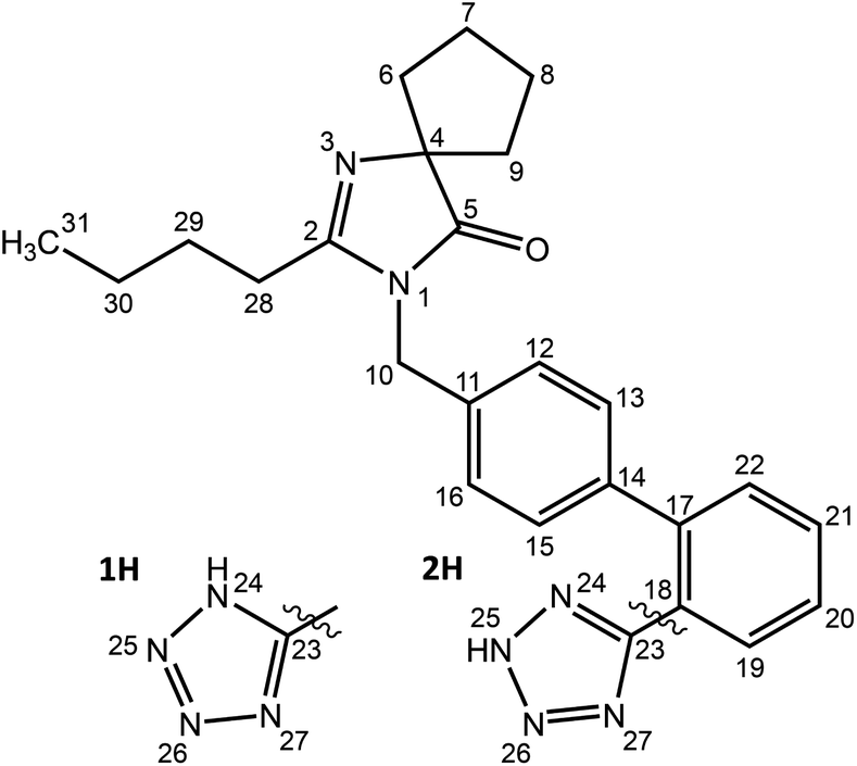

Scheme 1 Structure of irbesartan (IRB). There are two distinct tautomers of the tetrazole ring, labelled 1H and 2H.

Up to 5 independent simulation boxes were generated using random positions and orientations of either 100 1H or 2H molecules at low density (box dimension 6.5 × 6.5 × 6.5 nm³). Mixed simulations boxes (denoted IRB-1H2H) containing 50 1H and 50 2H molecules chosen randomly were also generated. High energy contacts were removed by steepest descent energy minimisation. This was followed by a pre-equilibration run in the constant-NVT ensemble for 500 ps, at 300 K and 1 bar. The simulation boxes were then compressed by applying relatively high temperature and pressure (500 K, 1000 bar) for 1 ns, without including long-range electrostatics, reducing the box dimension to ∼4 × 4 × 4 nm³. The systems were then equilibrated for 300 K and 1 bar for 10 ns in the constant-NPT ensemble with the long-range electrostatics included. Finally, data was acquired on the equilibrated systems during 200 ns production runs. Snapshots were taken every 400 ps, corresponding to 501 snapshots over each production run. See Fig. S1 of the ESI† for a schematic illustration of this process. Unless otherwise indicated, results are shown for the first model glass system.

Periodic boundary conditions were employed in three dimensions, and the equations of motion were integrated with a timestep of 2 fs for a total simulation time of 200 ns. Bonds to H atoms were constrained with the P-LINCS algorithm,^27,28 and the cutoff for electrostatic and van der Waals interactions was 1.2 nm. The Nosé–Hoover thermostat^29,30 and Parrinello–Rahman barostat^31,32 were used with coupling constants of 1.0 and 2.0 ps respectively, and a reference pressure of 1 bar (using isotropic pressure scaling).

The dependence of molecular diffusion on temperature was evaluated on IRB-1H (glass 1 model) by heating and then cooling from 250 K to 450 K and back, in intervals of 25 K. Two simulations were run for 200 ns at each temperature, the former for equilibration and the latter for data collection, with the simulation box at the end of each run used as the input for the next simulation. The same procedure was followed for a smaller number of simulations of IRB-2H and IRB-1H2H, where the systems were heated from 300–400 K in 50 K steps.

2.2 Prediction of NMR chemical shifts and spectra

Python scripts were used to pass the 501 snapshots from the MD simulation production runs to ShiftML2, and the H, C and N isotropic shieldings predicted together with their associated uncertainties. Shieldings, σ, were converted to chemical shifts, δ, ignoring any deviation of the referencing gradient from −1, i.e. δ = σ_ref − σ, using references values of 170.5, 31 and −168 ppm for ¹³C, ¹H and ¹⁵N respectively, in order to qualitatively align experimental and simulated spectra. (More quantitative referencing is difficult due to the distributions of shifts for a given site in both calculated and experimental data.) The chemical shifts for the 100 molecules were averaged over the snapshots, and synthetic spectra created by convolution with Gaussian or Lorentzian lineshape functions.

2.3 Analysis of MD simulations: molecular motion

The diffusivity of molecules in the simulation box, represented by the diffusion coefficient, D, is calculated from the mean-squared displacement (MSD) via the Einstein relation³³where r_i(t) are the atomic positions of a reference atom in the molecule. Provided that measurements are recorded over a sufficiently long time, D can be obtained from the gradient of the MSD with respect to time. As illustrated in Fig. S2 of the ESI,† plots of the MSD of the C11 atom vs. t are generally linear, with deviations at short time (when the motion is ballistic rather than diffusive) and at longer times (associated to the sliding time window used for data smoothing). Hence D was estimated from the gradient of the MSD between 10–175 ns.

The local reorientation of molecular segments was evaluated via the correlation function, C(t), of characteristic unit vectors in different parts of the molecule, including the butyl chain, and benzene and tetrazole rings. These were defined by vectors normal to the plane spanned by a set of three atoms (e.g. C28, C29 and C30 for the butyl chain). The decay of the resulting correlation functions can be characterised by an effective correlation time, τ_c,eff:

All the correlation functions corresponded to suggest unrestricted diffusion, i.e. the limiting value of C(∞) was taken to be zero, and the integration in eqn (2) was approximated numerically with Simpson’s rule. At lower temperatures, some correlation functions were truncated, cf. Fig. 1b, which would lead to minor underestimation of τ_c,eff.

2.4 Analysis of MD simulations: hydrogen bonding

Hydrogen bonds are typically characterised into broad categories of ‘strong’, ‘moderate’, and ‘weak’,^34,35 based on donor–acceptor distance, r_DA, and angle, θ_DHA. Jeffrey,³⁴ for example, proposes r_DA < 2.5 Å, θ_DHA > 175° for strong hydrogen bonds and 2.5 Å < r_DA < 3.2 Å, θ_DHA > 130° for moderately strong bonds. The GAFF force field used here represents hydrogen bonding through electrostatic terms, relying on AM1-BCC partial charges that have been fitted to a quantum chemical electrostatic potential. While the partial charge distribution will favour the linearity of hydrogen bonds at shorter distances, this purely electrostatic description is likely to be more effective for moderate and weaker strength H-bonds and less accurate for strong H-bonds.

Different cutoff parameters have been used in the limited literature on MD of amorphous drug materials. For example, the distance cutoff, r_HA (i.e. hydrogen acceptor distance, which will be ∼1 Å shorter than r_DA), chosen has varied between 2.45 Å,^36,37 2.5 Å,²² up to 3.5 Å.¹⁴ The choice of θ_DHA has been similarly varied, between a restrictive minimum angle of 145° used by Chelli et al.,^36,37 130°²² and down to 120°.^14,38

Here we have optimised the cutoff parameters directly on the predicted ¹H shift data for the tetrazole H. Python scripting was used to identify the hydrogen bonding environments in all the snapshots of a simulation using a given pair of r_HA and θ_DHA cutoff parameters. Simultaneously ShiftML2 was used to the predict the chemical shifts, giving rise to an overall distribution of shift values (total data in Fig. S12 of the ESI†). The two data sets were correlated, allowing the shift values to be separated into a distribution classed as hydrogen bonded and a distribution classed as non-H-bonded. As illustrated in Fig. S12,† a θ_DHA of about 130° neatly partitions the overall distribution into two roughly Gaussian distributions. Looser or tighter angular cutoffs clearly over-emphasise or under-emphasise the hydrogen bonded contribution respectively. The two distributions were fitted independently to Gaussian functions and χ² calculated between the sum of the two Gaussians and the total distribution. As shown in Fig. S13 of the ESI,† r_HA and θ_DHA were scanned in steps of 0.25 Å and 10° respectively in order to minimise χ². From this analysis, the cutoffs used below were θ_DHA ≥ 125° and r_HA ≤ 3.5 Å.

2.5 Experimental NMR

Crystalline irbesartan form A was obtained from Sigma-Aldrich. Amorphous samples were produced by heating the sample at ∼186 °C in an oven for 10 minutes, before immediate cooling in a refrigerator.

The ¹³C spectrum of amorphous IRB was obtained using a 400 MHz Bruker Avance III HD spectrometer and a 4.0 mm (rotor o.d.) magic-angle spinning (MAS) probe, at a MAS rate of 10 kHz. 2048 scans were acquired using ¹H cross-polarisation using a ramped 5 ms contact pulse and a recycle delay of 3 s. Proton excitation and decoupling used a nutation rate of 71.5 kHz. The spectrum obtained was indistinguishable from that of previous literature results,⁹ confirming that the amorphous form of this material is well defined.

The ¹H spectrum of amorphous IRB was obtained at 1 GHz (National Solid-State NMR Research Facility) at a MAS rate of 60 kHz. 4 scans were acquired and a recycle delay of 3 seconds was used. Proton excitation and decoupling used a nutation rate of 100 kHz.

3 Results

3.1 Analysis of molecular motion

Fig. 1 summarises molecular mobility in the simulation results as a function of temperature in terms of (a) molecular diffusion coefficients, D, and (b) rotational correlation functions for vectors in the molecular core and on the flexible butyl chain. There is a smooth evolution in D as the temperature increases, with a clear acceleration of this change above the glass transition temperature. Taken together with the excellent reproducibility of the results over heating and cooling, this strongly suggests that the initial models are good representations of an amorphous molecular solid; although the location of T_g is not clear cut, the overall transition from a glassy to a more dynamic material is being captured by the force field used. The relative “softness” of T_g is consistent with previous NMR relaxation data,⁹ which showed a smooth evolution of the relaxation times through the glass transition. As shown in Fig. S3 of the ESI,† the molecular diffusion in the mixed simulations lies between that of pure components.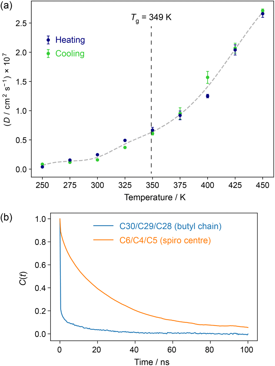

Fig. 1 (a) Mean diffusion coefficients averaged over all C11 atoms in IRB-1H simulations as a function of temperature. The total size of the “error bars” corresponds to the difference between values of D fitted from the first and second halves of time period used for analysis (10–175 ns). See Fig. S2 of the ESI† for the raw data. The grey dashed line is a spline fit to the mean of heating and cooling data points as a guide to the eye, and the vertical dashed line indicates the experimental value of T_g observed at a 10 °C min⁻¹ heating rate.³⁹ (b) Rotational autocorrelation functions of a characteristic vector in the butyl chain (blue) and the spiro carbon ring (orange) in IRB-1H simulations at 300 K (heating). The atom numbering used is in Scheme 1.

Analysis of correlation functions for vectors corresponding to different parts of the molecule, Fig. 1b, shows two broad behaviours; very fast dynamics in the butyl chain, and slower dynamics in the rest of the molecule; see Fig. S5 of the ESI† for further analysis of reorientational correlation times. Again, this is consistent with previous experimental relaxation data, which showed faster dynamics for the butyl chain than the aromatic core.⁹

The distance moved by molecules (illustrated in Fig. S4 of the ESI†) helps to contextualise the extent of motion. For example, even at 300 K (i.e. 50 K below T_g), the median molecular displacement over the course of the 200 ns simulation of IRB-1H is 13 Å (heating run). Although the overall distributions are highly reproducible, there is considerable range in the extent of translation in individual molecules, especially at higher temperatures, e.g. some molecules move less than 10 Å over 200 ns at 400 K, while others move over 60 Å. This heterogeneity is somewhat arguably obscured by the highly averaged data shown in Fig. 1. As previously, the dynamics changes only in extent either side of the glass transition, meaning that we cannot consider the disorder in the glassy solid as static, and it will be necessary to average over the MD trajectory to make meaningful comparisons with experimental NMR data.

3.2 ¹⁵N NMR

The importance of averaging over molecular motion of amorphous solids molecules solids at ambient temperature can be seen in Fig. 2. The range of chemical shifts spanned by a particular N site, shown as histograms in Fig. 2a for IRB-1H, are clearly far too broad to match the experimental spectrum, (d). Note that N–H bond lengths were fixed in the MD simulations, and so this variation is not simply a reflection of fast vibrational motion leading to unreasonable shift values. Averaging the shielding/shift for a given site over the snapshots of the simulation gives considerably narrower distributions, Fig. 2b and c for pure IRB-1H and IRB-2H respectively. As illustrated in Fig. S6 of the ESI,† these resulting synthetic spectra are highly reproducible between independent glass models. Given that the uncertainties on the ShiftML2 predictions, see Table S2 of the ESI,† are 10–15 ppm, there is reasonable agreement between positions of the peaks in the synthetic spectra and the experimental ¹⁵N spectrum of amorphous IRB. This is practically significant, because it was previously not possible to predict chemical shifts in the amorphous material using conventional NMR crystallography tools. The synthetic spectra show that the previous somewhat tentative assignment, based on shift values in other crystalline sartan materials, was reasonable.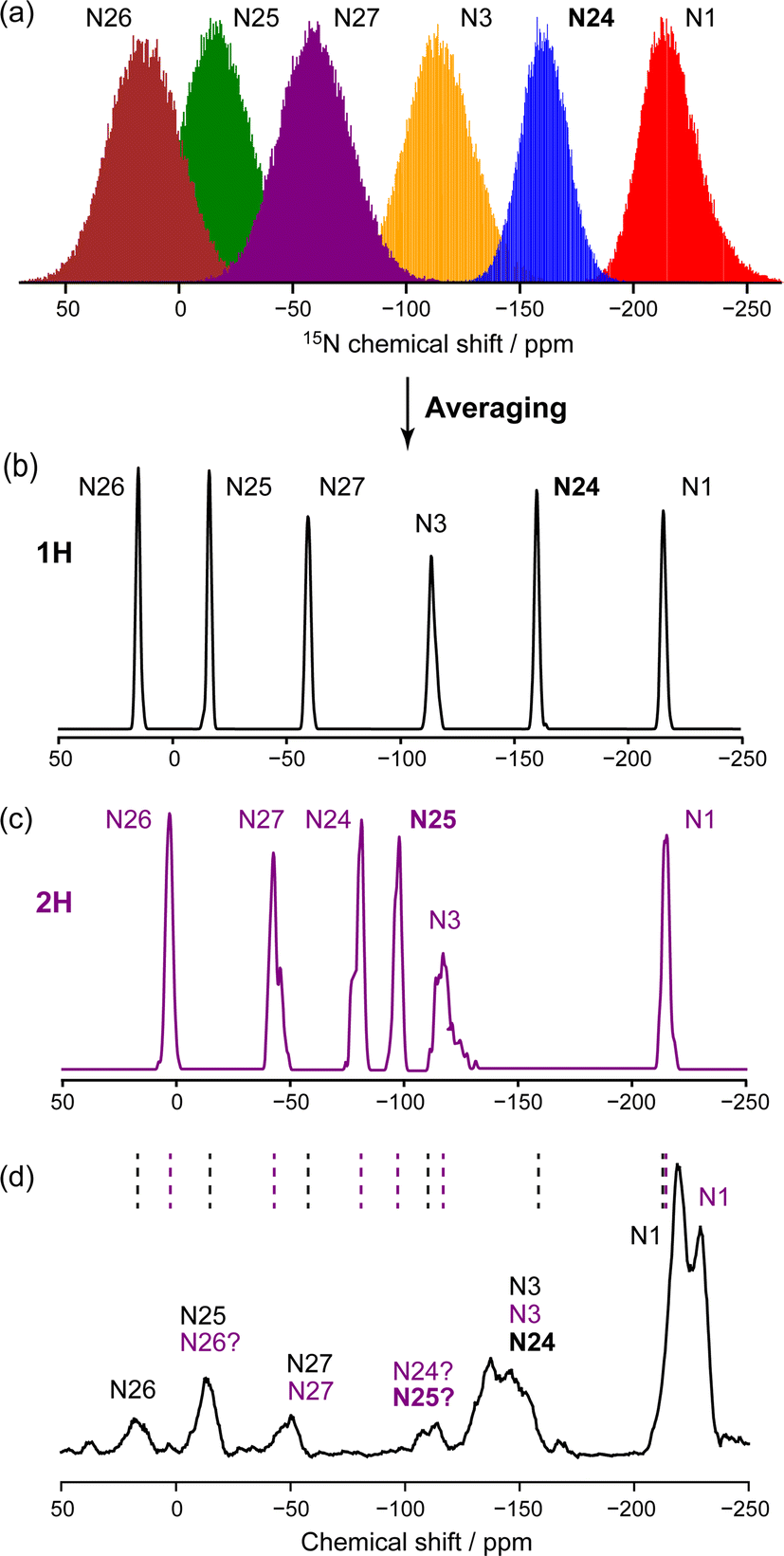

Fig. 2 (a) Raw distributions of the ¹⁵N chemical shifts for all 100 molecules and all 501 snapshots of an MD simulation of IRB-1H. Synthetic ¹⁵N spectra for (b) IRB-1H and (c) IRB-2H simulations after averaging the shift for each site over the snapshots, and using a 0.5 ppm Gaussian intrinsic lineshape. (d) Experimental ¹⁵N spectrum of amorphous IRB, adapted from data originally published in ref. 9. The dashed black and purple lines indicate the positions of the peak maxima in (b) and (c) respectively. The protonated nitrogens (N24 and N25 for 1H and 2H tautomers respectively) are highlighted in bold.

3.3 ¹³C NMR

Fig. 3 compares two approaches to predicting the spectrum of the amorphous IRB. Summing the spectra obtained from simulations of the pure tautomers gives a result that is indistinguishable from that of a simulation of a 50 : 50 mixture, especially after applying a realistic line-broadening. As well as confirming the reproducibility of the results, this confirms the appropriateness of characterising the behaviour of the pure tautomers

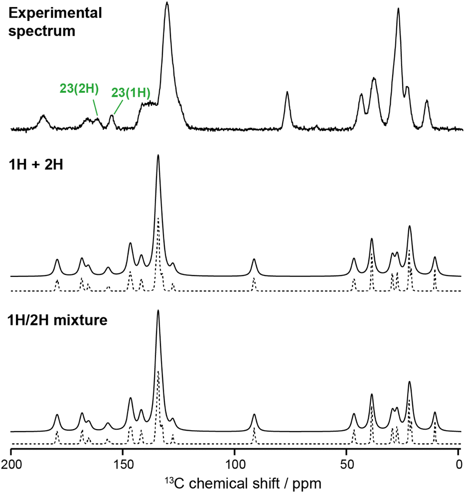Fig. 3 (Top) Experimental ¹³C spectrum of amorphous IRB and simulated ¹³C spectra obtained by (middle) adding results from separate MD simulations for 1H and 2H IRB tautomers and (bottom) from a simulation of a 50 : 50 1H : 2H mixed unit cell. The averaged shift values are convoluted with Lorentzian peaks with two different line widths: FWHM of 2 ppm (solid line), for visual matching with the experimental spectrum, and 0.2 ppm (dotted) to highlight the underlying lineshapes due to disorder. The labels highlight the C23 resonance, which differs significantly between the tautomers.

The predicted shift for the C4 site is about 10 ppm higher than observed in experiment. The average ShiftML2 uncertainty for the site (about 8.3 ppm) is the highest of the C sites (presumably reflecting the atypical azaspiro functionality). On the other hand, the ShiftML predictions agree well with DFT for a crystalline form (Fig. S8 of the ESI†), and this apparent discrepancy may reflect the simple approach to ¹³C referencing adopted; it would be typical in crystalline systems to establish referencing using a linear regression in which the shift-shielding gradient can deviate from −1.

The uniform 2 ppm Lorentzian line-broadening in Fig. 3 used to obtain a reasonable visual match with the experimental spectrum appears somewhat arbitrary. The intrinsic homogeneous linewidths were estimated using measurements of ¹³C , that is the decay of the ¹³C signal using a spin-echo to refocus inhomogeneous broadenings.⁴⁰ As shown in Fig. S9 of the ESI,† however, the values in the amorphous material were comparable to those in the crystalline material, implying little significant broadening by dynamic effects. (The dynamics observed in simulation are too fast to influence .) Overall we find that the simulations under-predict the linewidths seen experimentally by about 2 ppm for all the nuclei considered. As discussed below, magnetic susceptibility effects provide a possible explanation for such a uniform inhomogeneous broadening.

The MD simulations allow the molecular origin of difference in the C23 chemical shift between tautomeric forms to be probed. Fig. 4 shows the correlation between the ML-predicted shift for C23 and the torsion angle between the tetrazole and C23-containing rings. The plot for the 2H tautomer is unremarkable; the planar conformations of the two rings (0° and 180°) are avoided, with favourable twisted conformations at approximately ±50° and ±130°. The conformational behaviour of the 1H tautomer is strikingly different; the ±50° conformations are strongly preferred over ±130°, and a planar conformation of the rings is now strongly favoured. The avoidance of the ±130° conformations is due to a steric clash between the N24 and C15 hydrogens, and does not affect the average chemical shift (indicated by horizontal lines). In contrast, the planar conformation observed in 1H has a low chemical shift of about 150 ppm. Combined with a small electronic effect—the features ±50° and ±130° being on average ∼5 ppm lower for 1H—this explains the much lower average chemical shift for C23 observed in the 1H tautomer.

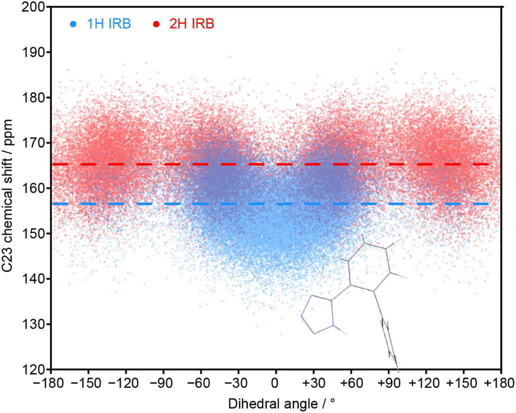Fig. 4 Relationship between the C23 chemical shift of IRB with the torsion angle of the tetrazole and the C23-containing ring (N24–C23–C18–C17 torsion) for every molecule and snapshot of the MD simulations for pure 1H and 2H tautomers. The average chemical shifts (averaged over time and all molecules) for each tautomer (dashed lines) matches the splitting of the C23 peaks in the amorphous ¹³C spectrum. The inset structure illustrates the favourable conformation associated with a zero dihedral angle (see Fig. S11 of the ESI† for the complete structure).

The unusual conformational distribution in the 1H tautomer suggests that there is an additional intramolecular interaction. The planar relative conformation of the tetrazole and adjacent aromatic ring (N24–C23–C18–C17) is correlated with a preferred conformation of the following key torsion angle (C18–C17–C14–C15) of approximately ±105° (see Fig. S10 of the ESI†). This corresponds to an overall conformation in which the tetrazole is directed towards the central aromatic ring (see Fig. S11†). This conformational preference has been confirmed by energetic profiling of gas phase molecules using DFT (see Fig. S19†).

3.4 ¹H NMR and analysis of hydrogen bonding

Fig. 5 also shows that there is negligible difference between ¹H spectra obtained by summing simulations or by simulating mixture. This is less obvious for ¹H given the significance of intermolecular interactions, especially hydrogen bonding, for ¹H spectra. The experimental spectrum, even at fast MAS and ultra-high magnetic field is relatively uninformative. Despite the high field, the resolution is unimproved compared to previous results at 499.7 MHz.⁹ In particular, the signal from the tetrazole H is extremely broad and featureless, highlighting the challenges of obtaining structural insight from the NMR data alone. But, having validated the MD simulations using dilute spin NMR, we can have some confidence in predicting the underlying behaviour of the ¹H shifts from the MD simulations.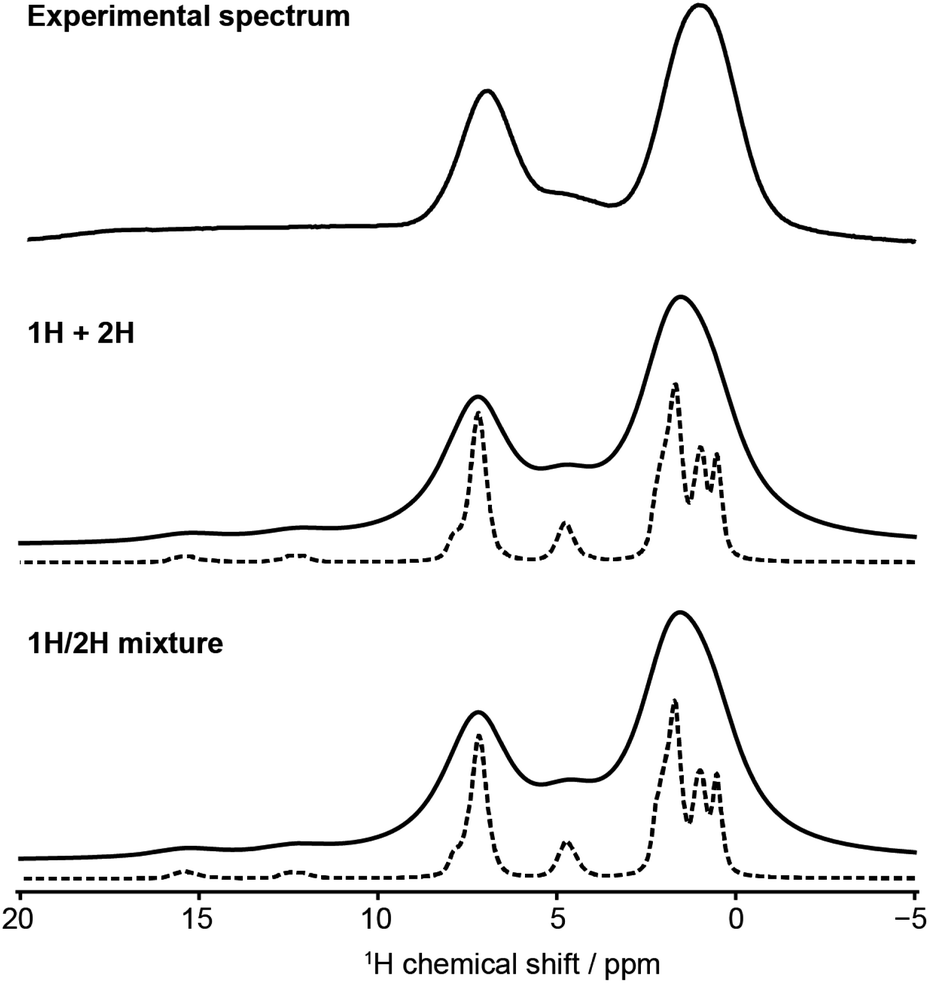

Fig. 5 (Top) Experimental ¹H spectrum of amorphous IRB obtained at 1 GHz and 60 kHz MAS spin rate, and simulated ¹H spectra obtained by (middle) adding results from separate MD simulations for 1H and 2H IRB tautomers and (bottom) from a simulation of a 50 : 50 1H : 2H mixed unit cell. The averaged shift values are convoluted with Lorentzian peaks with two different line widths: FWHM of 2 ppm (solid line), for visual matching with the experimental spectrum, and 0.2 ppm (dotted) to highlight the underlying lineshapes due to disorder.

Fig. 6 shows histograms of unaveraged ML-predicted shifts for the key tetrazole hydrogen (H24 or H25) for all snapshots and all molecules. The overall histograms (grey) are clearly bimodal, with two approximately Gaussian distributions corresponding to H-bonded vs. non-H-bonded hydrogens. There is a striking difference in the distributions for the two tautomers, with a significantly greater fraction of H-bonding in the 2H tautomer. Note, however, that the distributions overlap, i.e. if a site has a chemical shift of say 14 ppm, we cannot assign it to a hydrogen bonded or non-hydrogen bonded environment purely on the basis of chemical shift, not least because there are different distributions for the two tautomers. Given geometrical criteria for identifying hydrogen bonded sites, we can, however, determine whether a given H24/H25 can be classified as hydrogen bonded, and correlate these predicted shifts against hydrogen bond geometry. Hence we can tune the cutoff parameters directly on these distributions, using the methodology discussed in Section 2.4. Although there is no objective reason why the distribution should divide cleanly into two Gaussians, it is clear that the optimised angular cutoff θ_DHA ≥ 125° gives an excellent split of the overall distribution, and provides an objective NMR-driven route to classifying which tetrazole H atoms should be treated as H-bonded.

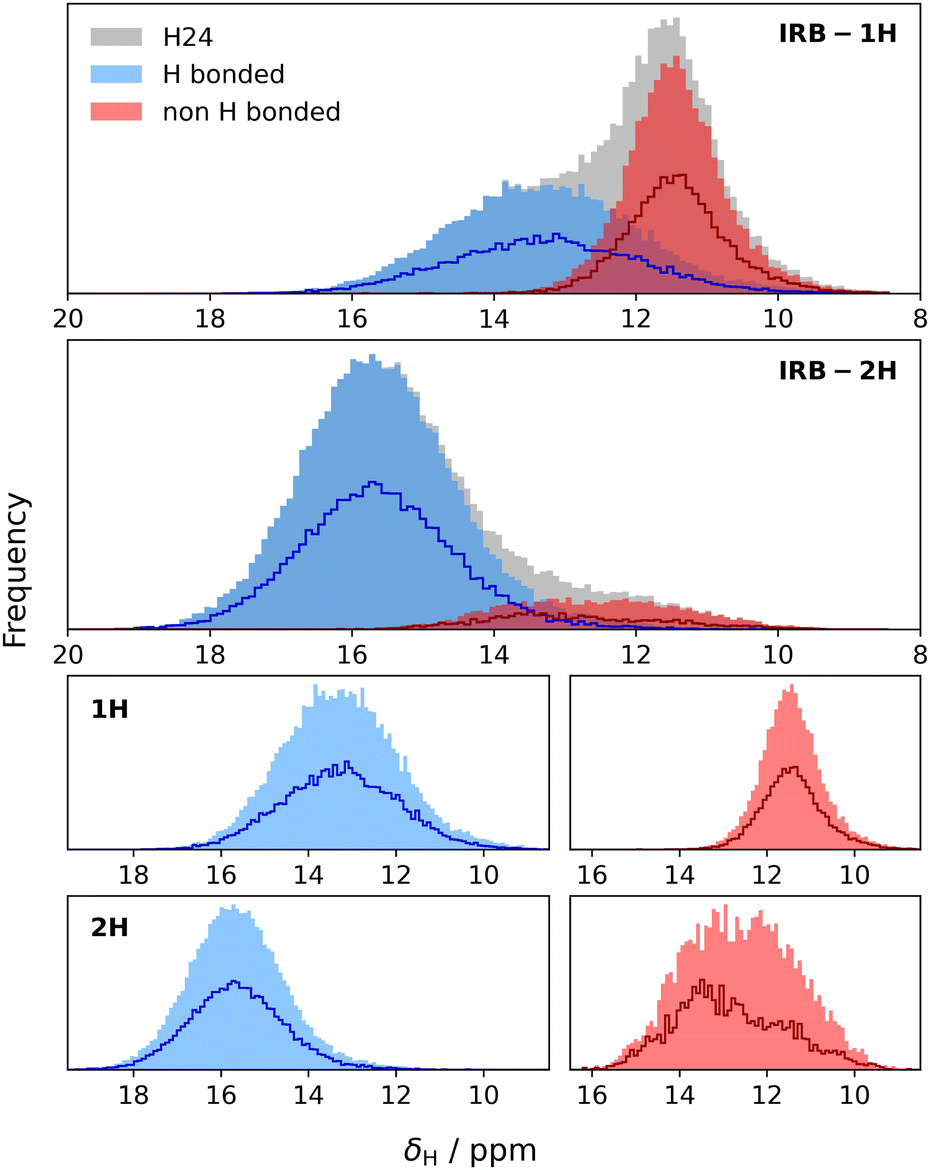Fig. 6 ShiftML2-predicted chemical shifts of all tetrazole H atoms for IRB-1H and IRB-2H from 501 frames of MD simulations at 300 K. The H atoms are classified into hydrogen-bonded (blue) vs. non-hydrogen bonded (red) based on an angular cutoff of 125° and distance cutoff of 3.5 Å. Darker outlines show the distribution of the chemical shifts for the corresponding components in the IRB-1H2H mixture. The four lower plots show each histogram separately for clarity.

As observed previously, there is little difference in the behaviour of a given tautomer depending on whether it is in its pure state or in a mixture. Indeed, the frequency distributions for the sites classified as hydrogen bonded (blue curves in Fig. 6) in the 50 : 50 mixture are simply half those of the pure material. There is a noticeable difference in the distributions of the non-H-bonded sites (red curves). This is consistent with the picture that the tetrazole H in 1H is largely involved with an intermolecular non-H-bonding interaction, while the tetrazole H in 2H is exposed to a wider variety of local environments (noting the greater range in shift values), and these differ between the pure material and the mixture.

Fig. 7 shows an analysis of the bonding environment of the key tetrazole hydrogen using these cutoff criteria for pure 1H, 2H and mixture simulations. As expected from the results in Fig. 6, the 2H tautomer has a much greater fraction of H-bonding. Given the relatively wide angular cut-off for hydrogen bonding, it is unsurprising that we find a number of cases where H24/H25 is hydrogen bonded to more than one acceptor atom (typically N), see Table S3 of the ESI† for some statistics, while Fig. S14–S18† examine how the ¹H shift depends on the geometry of the hydrogen bond and correlations between H bond angles and bond lengths. Such correlations are well known in the literature, as is the fact the overall chemical shift will reflect a combination of geometrical and electronic factors (there is an overall shift of about 2 ppm between the distributions of the two tautomers, Fig. S15†).

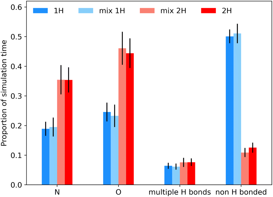Fig. 7 Proportion of simulation time spent by the tetrazole hydrogen in different hydrogen bonding environments, based on 501 snapshots, and averaged over all molecules in IRB-1H, IRB-2H and 50 : 50 mixture simulations at 300 K. The “mix 1H” and “mix 2H” columns refer to 1H and 2H molecules respectively in the mixed system. The H24/H25 environment at a given time is categorised into hydrogen bonded to N or O, not hydrogen bonded or hydrogen bonded to more than one acceptor (typically N), using the geometrical cutoffs for an H-bonded site of r_DA ≤ 3.5 Å and angle θ_DHA ≥ 125°. Error bars indicate ±2 standard errors from the averaging over 100 molecules.

4 Discussion and conclusions

The combination of ML-predicted chemical shifts and trajectories from MD simulations allows the chemical shifts in an amorphous drug material to be efficiently derived. The simulations show that there is significant dynamics, including at temperatures well below the glass transition, and averaging over multiple snapshots of MD trajectories is essential. Simulations over 200 ns were required for the orientational correlation functions, Fig. 1b, to decay to close to zero at 300 K. Under these conditions, the results from independent simulation boxes were highly reproducible. The systems are observed to behave as supercooled liquids, with the average spectra and hydrogen bonding frequencies for a given molecule/tautomer being largely independent of whether the simulation contained a single tautomer or a mixture.

The simulated spectra are narrower than experimental spectra by about 2 ppm. This will partly reflect residual effects of dipolar coupling (especially for ¹H). This additional linewidth is essentially inhomogeneous, rather than resulting from dynamic broadening. A plausible origin of the remaining difference in linewidth is bulk magnetic susceptibility (BMS) effects, i.e. the variation of bulk magnetic susceptibility, and hence the effective B₀, on the orientation with respect to the magnetic field. Magic-angle spinning partially averages this anisotropic effect, but additional linewidths of 1 ppm are typically encountered for materials that contain aromatic rings. Moreover, the average BMS shift at different locations in an amorphous material is likely to vary (in contrast to crystalline materials). Hence it is plausible that a large fraction of the difference between predicted and experimental linewidths can be explained by these effects.

Despite the intrinsic broadness of the experimental spectra, it is still possible to relate spectra and predictions. For the ¹⁵N spectra, the predictions help to validate the assignment of the experimental amorphous spectrum, which previously could only be tentatively made based on pooled shift values from crystalline materials. The predicted amorphous spectra allow assignments to be made without need for data from crystalline analogues.

A significant difference in ¹³C shift between tautomeric forms had been observed in the amorphous spectrum of IRB, but its physical origin could not be deduced from NMR. The MD simulations show that the tetrazole ring adopts significantly different conformations in the two tautomers; there is a favourable intramolecular interaction in the 1H tautomer that is not possible in the 2H tautomer. This difference in average molecular shape is also likely to explain the difference in molecular diffusivities of the two tautomers (see Fig. S3 of the ESI†). Understanding the origin of this behaviour would not be possible with “classical” approaches to NMR crystallography involving DFT calculations of a limited number of crystalline forms. Indeed, conformations observed in crystalline forms may not be representative of the distribution of conformational space occupied in amorphous materials—it is quite common for relatively high energy molecular conformations to be stabilised in individual polymorphs.^8,41,42 The combination of MD simulation to generate model amorphous glasses and ML-based shift prediction allows the connection between the NMR data and molecular behaviour to be explored in a thorough and unbiased fashion.

A similar pattern is observed from the ¹H NMR. Here the high frequency region of the ¹H NMR spectrum is sensitive to hydrogen bonding behaviour. Consistent with the degree of overall molecular mobility, the hydrogen bonding patterns are observed to be highly dynamic, and averaging over the MD trajectory is essential to make comparisons with experimental behaviour. Although difficult to observe experimentally, the average shift for the tetrazole hydrogen is directly linked to the fraction of time spent in hydrogen bonds, with the lower shift for the 1H tautomer reflecting the significant fraction of time spent in the conformation stabilised by a non-hydrogen bonding intramolecular interaction.

It is important to recognise that the correlations between NMR chemical shifts and molecular behaviour are being obtained through different approximations. The predicted shifts are obtained from an ML model trained on DFT predictions (themselves approximations). Hence the correlations between NMR observables and geometrical parameters (Fig. S15 and S16 of the ESI†) are “only” effectively read outs from the ML model. But given the effectiveness of the ML model in predicting experimental shifts,²¹ and the results presented here, the ability to probe the dependence of chemical shift on local geometry is extremely valuable, especially if MD is being used to generate an ensemble of plausible local environments. The fact that we can efficiently predict chemical shifts for a large numbers of sites allowed us to derive, for example, system-specific cutoffs for hydrogen bonded vs. non-hydrogen sites, in a way that is not possible by pooling results from crystalline forms.

NMR provides a uniquely powerful probe of local environments, with ¹³C shifts being particularly sensitive to molecular conformation, and ¹H shifts to inter/intramolecular interactions. But the degree of molecular mobility in amorphous forms of small molecular drugs, makes it difficult to rationalise the experimental data in the absence of simulation. The fact that the experimental results can be rationalised by simulation helps in turn to validate the simulation methodology, establishing the synergy between experiment and computation.

Data availability

Data for this article is available at Durham Collections at https://doi.org/10.15128/r2m900nt43g.

Author contributions

Jamie L. Guest: investigation, visualisation, writing – review & editing. Esther A. E. Bourne: investigation, visualisation, writing – review & editing. Martin A. Screen: software. Mark R. Wilson: methodology, writing – review & editing. Tran N. Pham: funding acquisition, supervision. Paul Hodgkinson: funding acquisition, conceptualisation, supervision, writing – original draft.

Conflicts of interest

There are no conflicts to declare.

Acknowledgements

JLG is co-funded by an EPSRC Industrial CASE award and GSK. MS thanks the Engineering and Physical Sciences Research Council and AstraZeneca for studentship funding via the Soft Matter and Functional Interfaces Centre for Doctoral Training (EP/S023631/1). This work directly benefitted from networking/training activities run by the Collaborative Computing Project for NMR Crystallography, funded by EPSRC grant EP/T026642/1. The authors wish to thank Durham University for computer time on its high performance computer, hamilton8. The UK High-Field Solid-State NMR Facility used in this research was funded by EPSRC and BBSRC (EP/T015063/1), as well as, for the 1 GHz instrument, EP/R029946/1.

Notes and references

1. C. A. Lipinski, F. Lombardo, B. W. Dominy and P. J. Feeney, Adv. Drug Delivery Rev., 1997, 23, 3–25.
2. C. A. Lipinski, J. Pharmacol. Toxicol. Methods, 2000, 44, 235–249.
3. Disordered pharmaceutical materials, ed. M. Descamps, Wiley-VCH, Weinheim, 2016.
4. R. Laitinen, K. Löbmann, C. J. Strachan, H. Grohganz and T. Rades, Int. J. Pharm., 2013, 453, 65–79.
5. B. C. Hancock and M. Parks, Pharm. Res., 2000, 17, 397–404.
6. L. Yu, Adv. Drug Delivery Rev., 2001, 48, 27–42.
7. S. Thakral, M. W. Terban, N. K. Thakral and R. Suryanarayanan, Adv. Drug Delivery Rev., 2016, 100, 183–193.
8. M. Skotnicki, D. C. Apperley, J. A. Aguilar, B. Milanowski, M. Pyda and P. Hodgkinson, Mol. Pharmaceutics, 2016, 13, 211–222.
9. M. Skotnicki and P. Hodgkinson, Solid State Nucl. Magn. Reson., 2022, 118, 101783.
10. NMR Crystallography, ed. R. K. Harris, R. E. Wasylishen and M. J. Duer, John Wiley & Sons, Incorporated, Hoboken, 2nd edn, 2012.
11. P. Hodgkinson, Prog. Nucl. Magn. Reson. Spectrosc., 2020, 118–119, 10–53.
12. M. Descamps and J.-F. Willart, in Disordered pharmaceutical materials, ed. M. Descamps, Wiley-VCH, Weinheim, 2016, ch. 1, pp. 1–56.
13. J. A. Bama, E. Dudognon and F. Affouard, J. Phys. Chem. B, 2021, 125, 11292–11307.
14. T.-X. Xiang and B. D. Anderson, Mol. Pharmaceutics, 2013, 10, 102–114.
15. F. Ngono, G. J. Cuello, M. Jiménez-Ruiz, J. F. Willart, M. Guerain, A. R. Wildes, A. Stunault, C. M. Hamoudi-Ben Yelles and F. Affouard, Mol. Pharmaceutics, 2020, 17, 10–20.
16. J. Gerges and F. Affouard, J. Pharm. Sci., 2020, 109, 1086–1095.
17. A. Schahl, I. C. Gerber, V. Réat and F. Jolibois, J. Phys. Chem. B, 2021, 125, 158–168.
18. V. Erastova, I. R. Evans, W. N. Glossop, S. Guryel, P. Hodgkinson, H. E. Kerr, V. S. Oganesyan, L. K. Softley, H. M. Wickins and M. R. Wilson, J. Am. Chem. Soc., 2024, 146, 18360–18369.
19. F. M. Paruzzo, A. Hofstetter, F. Musil, S. De, M. Ceriotti and L. Emsley, Nat. Commun., 2018, 9, 4501.
20. C. J. Pickard and F. Mauri, Phys. Rev. B, 2001, 63, 245101.
21. M. Cordova, E. A. Engel, A. Stefaniuk, F. Paruzzo, A. Hofstetter, M. Ceriotti and L. Emsley, J. Phys. Chem. C, 2022, 126, 16710–16720.
22. M. Cordova, P. Moutzouri, S. O. Nilsson Lill, A. Cousen, M. Kearns, S. T. Norberg, A. Svensk Ankarberg, J. McCabe, A. C. Pinon, S. Schantz and L. Emsley, Nat. Commun., 2023, 14, 5138.
23. D. Van Der Spoel, E. Lindahl, B. Hess, G. Groenhof, A. E. Mark and H. J.C. Berendsen, J. Comput. Chem., 2005, 26, 1701–1718.
24. M. J. Abraham, T. Murtola, R. Schulz, S. Páll, J. C. Smith, B. Hess and E. Lindahl, SoftwareX, 2015, 1–2, 19–25.
25. J. Wang, R. M. Wolf, J. W. Caldwell, P. A. Kollman and D. A. Case, J. Comput. Chem., 2004, 25, 1157–1174.
26. A. Jakalian, D. B. Jack and C. I. Bayly, J. Comput. Chem., 2002, 23, 1623–1641.
27. B. Hess, H. Bekker, H. J. C. Berendsen and J. G. E. M. Fraaije, J. Comput. Chem., 1997, 18, 1463–1472.
28. B. Hess, J. Chem. Theory Comput., 2008, 4, 116–122.
29. S. Nosé, Mol. Phys., 1984, 52, 255–268.
30. W. G. Hoover, Phys. Rev. A, 1985, 31, 1695–1697.
31. M. Parrinello and A. Rahman, J. Appl. Phys., 1981, 52, 7182–7190.
32. S. Nosé and M. Klein, Mol. Phys., 1983, 50, 1055–1076.
33. M. P. Allen and D. J. Tildesley, in Computer simulation of liquids, Oxford University Press, Oxford, 2nd edn, 2017, ch. 2, pp. 74–75.
34. G. A. Jeffrey, An Introduction to Hydrogen Bonding, Oxford University Press, New York, 1997, pp. 11–14.
35. T. Steiner, Angew. Chem., Int. Ed., 2002, 41, 48–76.
36. R. Chelli, P. Procacci, G. Cardini, R. G. Della Valle and S. Califano, Phys. Chem. Chem. Phys., 1999, 1, 871–877.
37. R. Chelli, P. Procacci, G. Cardini and S. Califano, Phys. Chem. Chem. Phys., 1999, 1, 879–885.
38. K. Mazeau and L. Heux, J. Phys. Chem. B, 2003, 107, 2394–2403.
39. M. Skotnicki, B. Jadach, A. Skotnicka, B. Milanowski, L. Tajber, M. Pyda and J. Kujawski, Pharmaceutics, 2021, 13, 118.
40. G. De Paëpe, A. Lesage and L. Emsley, J. Chem. Phys., 2003, 119, 4833–4841.
41. A. J. Cruz-Cabeza and J. Bernstein, Chem. Rev., 2014, 114, 2170–2191.
42. A. J. Cruz-Cabeza, S. M. Reutzel-Edens and J. Bernstein, Chem. Soc. Rev., 2015, 44, 8619–8635.

---

Footnote

† Electronic supplementary information (ESI) available. See DOI: https://doi.org/10.1039/d4fd00097h

---