Robust regression: An introduction

Abstract

Analytical scientists use regression methods in two main areas. Calibration graphs are used with the results of instrumental analyses to obtain concentrations from test samples. Graphical methods are used to evaluate the results obtained when two methods, often a novel one and a reference one, are compared by applying them to the same set of test materials. In either case outliers or suspect results may occur, and exert big effects on the plotted regression line and the results derived from it. Robust methods are well suited to tackling such situations. Here some of the underlying ideas are summarised: later briefs will describe some more of the many approaches available.

---

Calibrations and comparisons

There are several big differences between these two applications of regression. A calibration experiment uses a modest number of calibrators (standards, ∼6–10 of them), their concentrations spread evenly across the range of interest. One y-value (i.e. the experimental signal) is plotted for each standard x-value (concentration). It is often assumed that only y-direction errors are present, and that such errors are normally distributed and are similar at all values of x. These assumptions are not essential (see Technical Briefs 10 and 27), but they simplify the calculation of the regression line.

In a comparison or validation experiment there may be a large number of test samples, especially in clinical chemistry where many specimens are often available and validation is crucial. There might thus be more than one y-value for a given x-value. Both x- and y-values will clearly have variation between samples and experimental errors: these may not be uniform over the concentration range studied, or have a normal distribution. These differences, highlighted in the example in Table 1, must affect the ways in which the results of the two types of experiment are evaluated statistically.

An example

Table 1 Results from a calibration experiment

x	0	2	4	6	8	10	12	14	16	18
y	0.03	0.21	0.40	0.58	0.84	1.01	1.20	1.57	1.63	1.80

---

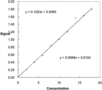
Point (14, 1.57) seems suspect, especially when the results are plotted (Fig. 1). The conventional least squares method gives the equation for the line through all the points as y = 0.1023x + 0.0065. This line looks inappropriate, as the effect of the suspect point is that almost all the other points lie below the fitted line. If we omit the suspect point, the least squares equation is y = 0.0999x + 0.0124. This line provides a better fit to all the points except for (14, 1.57). Using the two lines to find the concentration of a test sample giving a signal (y-value) of 1.40 units, the concentrations obtained are 13.62 units when all 10 points are used, and 13.89 units when the suspect value is omitted.

Fig. 1 Regression lines plotted with (continuous line) and without (dotted line) the inclusion of a suspect point.

This 2% difference is probably not very concerning to many analysts: but the standard deviations of the concentrations (see Technical Brief 22) are found to be 0.57 when all ten points are included, and only 0.22 if just nine points are used. So the choice of the best line makes a real difference to the estimated quality of the result.

This presents us with a dilemma. Common sense and wishful thinking suggest that the suspect point should be omitted. But probability theory shows that results very different from the expected ones must occur occasionally. So if there is no evidence of gross errors maybe the suspect measurement should be retained. Just as when suspect values occur in sets of replicate measurements, robust methods are of substantial value in regression applications.

Tackling the problem

One solution to such dilemmas lies in the use of median-based methods. The median of a data set is resistant (i.e. robust) towards the extreme values of the set, and Theil's Incomplete Method uses the median to plot regression lines. In our example the points on the graph are numbered 1, 2, etc in order of increasing x-value, and the slopes of the lines joining the pairs of points 1 and 6, 2 and 7, etc are calculated. (With an odd number of points the middle one is ignored). There are thus five slope estimates, and their median is taken as the slope of the line. This slope, used with the coordinates of each point, provides ten estimates of the intercept, and their median is taken as the true intercept. This method gives the equation of the line as y = 0.099x + 0.019, a result very similar to the one obtained when the least squares method is applied after rejection of the suspect point. Theil's Incomplete Method is simple and does not assume any particular distribution of measurement errors (i.e. it is non-parametric) or that all the errors lie in the y-direction. Despite these merits the method has not been much used in analytical chemistry though in the UK, the Department of Environment, Food and Rural Affairs recommends it for plotting the levels of critical atmospheric pollutants against time.

One obvious question is – how many suspect points can a given regression method tolerate before the slope and intercept of the calculated line are changed? The fraction of the n points that can be tolerated as outliers is known as the breakdown point of the method. Common sense and theory show that its maximum possible value is 0.5 (50%). Least squares results are affected by even one suspect point, so its breakdown point is (strictly) 1/n but effectively zero. Simulations show that the Theil Incomplete Method can tolerate one outlier if n ≥ 6, and 2 outliers if n ≥ 10. This would be adequate for many analytical calibration graphs.

The more complex Theil Complete Method uses all n(n − 1)/2 possible pairwise slopes of the lines from the n points to find the median slope, and the related method due to Passing and Bablok is very widely used in method comparison studies in clinical chemistry. It again uses all the pair-wise slopes to provide the median slope estimate, but with two refinements. It takes into account that when many specimens are studied using two methods, two or more of them may have the same x-values, thus giving pairwise slopes of ±∞. Moreover if suspect points arise on the graph there may be some negative slope values from individual pairs. The method takes this into account in a way which means that the x- and y-values, both subject to variation, can be interchanged without affecting the result. Normally distributed data in the x- or y-direction are not assumed, nor is it necessary that the experimental variations are similar at different analyte levels, though the ratio of the x- and y-variances should be about the same at all concentrations. It is assumed that there is a linear relationship between x and y, a condition that may not always arise in analytical work. These median based methods can be extended to give confidence limits for the slope and intercept of the regression line. In method comparison studies this allows the detection of significant differences from the ideal values of 1 and 0, respectively.

Available software

Application of these methods requires reliable statistical software. Several established programs provide Passing–Bablok calculations. Other commercially-available programs provide similar facilities as Microsoft Excel® add-ins. Theil's Incomplete Method is also very readily executed using Excel functions.

Further reading

The best-known text is Robust Regression and Outlier Detection by PJ Rousseuw and AM Leroy (John Wiley, 1987) but it is not easy reading, and is somewhat outdated. The Passing–Bablok method is summarised by its two originators in Journal of Automatic Chemistry, vol. 7, 1985, pp 74–79.

This Technical Brief was prepared by Professor James N Miller for the Statistical Sub-Committee of the Analytical Methods Committee.

---