Comparison of principal components regression, partial least squares regression, multi-block partial least squares regression, and serial partial least squares regression algorithms for the analysis of Fe in iron ore using LIBS

Abstract

The objective of the current research was to compare different data-driven multivariate statistical predictive algorithms for the quantitative analysis of Fe content in iron ore measured using Laser-Induced Breakdown Spectroscopy (LIBS). The algorithms investigated were Principal Components Regression (PCR), Partial Least Squares Regression (PLS), Multi-Block Partial Least Squares (MB-PLS), and Serial Partial Least Squares Regression (S-PLS). Particular emphasis was placed on the issues of the selection and combination of atomic spectral data available from two separate spectrometers covering 208–222 nm and 300–855 nm ranges, which include many of the spectral features of interest. Standard PLS and PCR models produced similar prediction accuracy, although in the case of PLS there were notably less latent variables in use by the model. It was further shown that MB-PLS and S-PLS algorithms which both treated available UV and VIS data blocks separately, demonstrated inferior performance in comparison with both PCR and PLS.

---

1. Introduction

Laser-Induced Breakdown Spectroscopy (LIBS) is a well-established analytical technique used for the quantitative analysis of a wide range of materials in many industrial and scientific applications. Examples may be found in some recent review articles.^1–3

The use of multivariate data analysis algorithms to interpret LIBS data sets has recently received a great deal of attention. In particular, such techniques as Principal Components Analysis (PCA) have been applied to material classification and identification,^4–6 while Principal Components Regression (PCR)^7,8 and Partial Least Squares Regression (PLS)^5,6,9 have proven successful in quantitative analysis. As LIBS data normally spans a spectral range of tens or hundreds of nanometres recorded with the use of a Czerny–Turner or an Echelle spectrometer, it is logical to seek a data-driven analysis algorithm that optimally utilises all the available spectral bandwidth to establish the strongest possible correlations between the spectral data and elemental composition. This is generally done by formulating a predictive model based on reducing the dimensionality of a data set of input raw spectral variables to a limited number of latent variables (or principal components in the case of PCR) in a spectral matrix X in such a way that they robustly correlate with the known concentrations y of the species analysed. It has been demonstrated that the use of data-driven multivariate statistical analysis techniques makes possible robust quantitative elemental analysis of species which LIBS normally struggles with, such as phosphorous,⁸ and even the prediction of material physical parameters which are not directly related to single species' elemental composition, for example, loss on ignition.¹⁰

The question of selecting the most suitable data-driven multivariate statistical analysis algorithm from a number of available options remains. Generally PLS is expected to perform slightly better than PCR, as the former is able to better cope with the problem which arises when significant changes in the analyte concentration give rise to only small variations in X, and also if there is a high degree of spectral interferences in the data. In an extreme case some important information can be interpreted by PCR as noise¹¹ and discarded. Further it is not necessarily clear which method should be chosen if there is data available from multiple spectrometers, especially if the spectra differ by dimensions, resolution and recorded intensity levels. It is expected that if two datasets (based on measurements of the same material with different spectrometers) are available for analysis, it is best to add them together to form an extended spectral matrix X, than, for example, use a multi-block regression analysis.¹² However, there is no guarantee that a combined block will provide better results compared to one of the single original blocks. For instance, the improvement can be compromised by the increased noise coming from the additional X matrix (block), or there simply may not be much useful information contained in it relative to the analyte. Also, it has been recently demonstrated that S-PLS, a multi-block analysis technique, is nevertheless capable of achieving the same or better results as PLS when analysing a combination of MIR and NIR spectra.^13,14

The LIBS data used in this study consisted of two blocks, which are referred to as UV (covering the range from 208 nm to 222 nm) and VIS (covering the range from 300nm to 855nm), which were collected using a Czerny–Turner spectrometer and an Echelle spectrometer respectively. Both spectrometers were fitted with intensified multichannel detectors. As PCR and PLS both use a single X block, three different analysis options were investigated. In the first case the data available from two spectrometers were put together to form a single extended X matrix. In other two cases the X matrix contained the data originating from only one of the spectrometers, taking either the UV or the VIS data as the X matrix.

MB-PLS is an extension of the standard PLS method and it is similar to PLS except that MB-PLS contains all measured variables into several blocks according to some predetermined criterion or a priori knowledge of the measurement or process.^15–17 Unlike the standard PLS, the MB-PLS operates with super scores and super weights obtained from multiple blocks and uses those for modelling and subsequent prediction. With S-PLS the data is treated as multiple X blocks separately in a serial mode, allowing the use of a different number of latent variables for modelling each data block.¹⁸

The aim of this present study was to compare the accuracy of analysis for Fe content in an iron ore matrix by applying the PCR, PLS, MB-PLS, and S-PLS algorithms to LIBS data sets. The emphasis is made on finding the optimal analytical strategy for the case when the spectral data is available is numerous blocks, which may or may not come from separate spectrometers. While the first two algorithms have been extensively used in LIBS for elemental analysis of a range of species, to our knowledge there are no reports of the use of the S-PLS or MB-PLS to analyse atomic spectral data. As the PCR, PLS, MB-PLS and S-PLS multivariate statistical algorithms have already been successfully applied to the analysis of NIR and MIR spectra, it seemed useful to investigate whether MB-PLS and S-PLS are useful for analysis of LIBS data

2. Theory

2.1 Principal components regression

PCR decomposes the predictor block X (n × p), using a selected number of principal components, so that important features of X are retained in a truncated matrix T:

X = TP^T + E (1)

In this case n is the number of samples measured and p is the number of pixels corresponding to the LIBS spectra. E is the matrix of residuals, the columns of matrix T are the scores and the columns of P are the loadings that linearly relate the principal components to the ‘raw’ spectral data. The scores and loadings are subsequently used to compute regression coefficients b for prediction of the unknown response vector ŷ (n × 1), in this case being the predicted concentration of the species of interest in each sample:

ŷ = Xb (2)

A training data set is used to generate the model in a calibration phase and a separate validation data set is used to evaluate the performance of the predictive model. Details of the implementation of PCR including the SVD factorisation and NIPALS algorithm are given by Jørgensen and Goegebeur.¹¹

2.2 Partial least squares regression

In contrast to PCR, PLS uses a selected number of latent variables to decompose both the predictor block X (n × p) and the response vector y (n × 1). This leads to two equations:

X = TP^T + E (3)

y = Tq^T + f (4)

Here q is the loading vector for y, and f is a vector of residuals for y. Predicted response vector ŷ is computed from the following linear equation, where b is an array of regression coefficients:

ŷ = Xb (5)

Separate training and validation data sets are used for calibration and evaluation of model predictive performance. Details on the implementation of the SIMPLS PLS algorithm used in this study are given by deJong.¹⁹

2.3 Multi-block partial least squares regression

MB-PLS is an extension to the standard PLS algorithm with the main difference being that (in our case) two predictor blocks X₁ (n × p₁) and X₂ (n × p₂) are used to model one response vector y (n × 1).

X₁=TP^T₁ + E₁ (6)

X₂=TP^T₂ + E₂ (7)

y = Tq^T + f (8)

Here p₁ and p₂ stand for the number of data points (pixels) in spectral blocks X₁ (UV) and X₂ (VIS), and T is a matrix of super scores, which contains the scores of predictor blocks X₁ and X₂.

Two variations of MB-PLS algorithms have been reported in literature. One version uses the block scores to calculate the loadings and residuals,¹⁵ while the second version uses the super-scores.¹⁷ The algorithm used in the present study was based on the latter version. In the calibration phase, block loadings and weights as well as super weights were computed from X₁, X₂, and y, and stored for prediction. The predicted response ŷ was estimated from the predictor data X₁ and X₂ corresponding to the unknown samples as well as the calibration loadings and weights, see Westerhuis et al.¹⁷ and Chong and Lee²⁰ for implementation details.

2.4 Serial partial least squares regression

In S-PLS, predictor blocks X₁, X₂, and response vector y are formed using the following relationships:

X₁=T₁P^T₁ + E₁ (9)

X₂=T₂P^T₂ + E₂ (10)

y = T₁q^T₁+T₂q^T₂ + f (11)

Here T_i and P_i are correspondingly the scores and the loadings for the predictor block X_i, and q_i is the loading vector for y. E_i and f are the residuals for X_i and y. Prediction was performed using the following linear model, where b₁ and b₂ are the regression coefficients for predictor blocks X₁ and X₂:

ŷ = X₁b₁ + X₂b₂ (12)

The major difference between the S-PLS and the MB-PLS algorithms is that in the former method decomposition of the predictor blocks (reduction of data dimension) is performed in a serial mode, and it is thus possible to use a different number of latent variables for blocks X₁ and X₂. Details on the implementation of the S-PLS algorithm used in this study are given by Felicio et al.¹³ and Berglund and Wold.¹⁸

3. Experimental

3.1 Laboratory setup

Fig. 1 shows a schematic diagram of the experimental setup used in this study. The fundamental output of a Q-switched Nd:YAG laser (Quanta-Ray INDI, Spectra Physics), pulse duration 5–8 ns, operating at 20 Hz was directed using steering mirrors and focused onto the sample surface with a 200 mm FL plano-convex lens. The beam was attenuated using the combination of a Brewster plate polariser and a half-wave plate. A constant laser-pulse energy of 40 mJ was used for this study.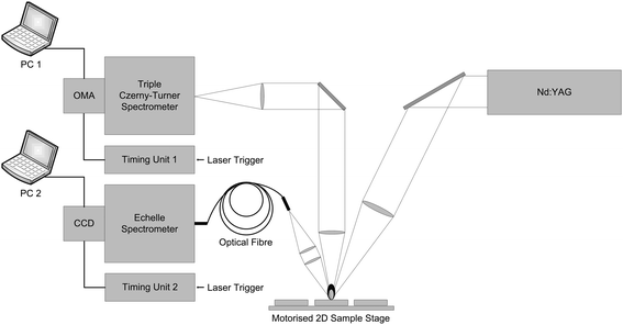

Fig. 1 Schematic diagram of the experimental setup.

The UV and VIS components of the LIBS plasma emission were collected by two sets of imaging optics and delivered to two separate spectrometers. A combination of two fused silica 100 mm FL, 25 mm diameter plano-convex lenses was used to collect, collimate and deliver UV emission to the triple Czerny–Turner spectrometer (Spex 1877C). This spectrometer was tuned to cover the 208 nm to 222 nm spectral range. The Spex spectrometer was equipped with a gated and intensified linear photodiode array detector (PDA, 1024 pixels long) which was controlled using an optical multi-channel analyser (OMA, Princeton Instruments ST-120 controller) and a PG-200 gate pulse generator.

A 100 mm FL plano-convex lens of 25 mm diameter sampled and collimated the VIS LIBS plasma emission and a second similar lens was used to focus the light into a 200 μm core optical fibre. The fibre was connected to the Echelle spectrometer (Spectra Pro HRE Echelle, Princeton Instruments) equipped with gated intensified CCD detector (1024 × 1024 pixel array, PI-MAX Princeton Instruments). The spectrometer nominally covers the 200–1000 nm range; however, due to the limitations of the optical components used in the experiment reported, the interval from 300 nm to 855 nm was used for the analysis. Both the PDA and ICCD detectors were externally triggered by the laser and set to 0.8 μs gate width and 2 μs gate delay between the laser Q-switch and acquisition start. The data has been collected simultaneously with the two detector systems. The detectors were triggered independently and not synchronised with each other.

3.2 Samples

The sample set used in this study has been previously described by Yaroshchyk et al.¹⁰ The sample set consisted of ring-milled and mechanically pressed iron ore pellets. The raw material was obtained from five different iron ore bodies. A total of 63 original samples with Fe ranging from 12.6 to 67.9% were used for model calibration, while another 60 original samples with Fe ranging from 14.2 to 67.9% were available for model validation. Their sub-samples were sent for XRF elemental analysis, with the results used as reference concentration values. All of the original samples were split in two resulting in a calibration set of 126 and validation set of 120 sub-samples. The splitting has been done mainly in order to double the size of the datasets, and it also provided easy means of monitoring the precision of measurements. A motorised sample-stage accommodating up to 105 pressed pellets was used to position the samples under the laser beam. A pair of stepper motors moved the stage in the orbital pattern under the control of a National Instruments MID-7604 controller operated using LabView software.

3.3 Data pre-treatment

Our previous work had shown the initial data pre-treatment to have a significant effect on the performance of the multivariate statistical analysis algorithms when applied to LIBS data.¹⁰ For every sub-sample used in this study a total of 50 spectra were collected. Each of those spectra was an average spectrum recorded with 40 and 50 laser shots for the OMA and PI-MAX detectors respectively. The UV and VIS data blocks were treated separately. Firstly a dark-noise background spectrum was subtracted from each of the laser-shot averaged data. Then an automatic filtering routine was employed to remove outlying spectra based on the integrated total energy of the spectral data (TE_i). Spectra with TE greater that 2 standard deviations from the mean for those 50 spectra were excluded from the spectral data set to be analysed. Here TE_i is defined as:Where I_ji was the counts in energy channelj for spectrumi. Each of the retained spectra were subsequently normalised to its total integrated energy TE_i. Depending on the analysis algorithm employed, the spectral data was collated into a single predictor block X or used as separate predictor blocks, X₁ and X₂. The X blocks have not been separately scaled prior to the concatenation. The MATLAB software equipped with the Statistics Toolbox has been used for all computations reported in this study.

4. Results and discussion

4.1 Calibration

For all methods reported in this study, a global sample dataset, y, comprising of 126 sub-samples originating from the five different ore bodies was used for model calibration. Separate global dataset, y^val, consisted of 120 sub-samples. The number of latent variables (or principal components in case of PCR) was chosen by performing the 10-fold cross-validation based on the metric of minimal mean squared error of cross-validation (MSECV):

The remaining subset y^val was used to provide an independent validation of the model with the metric of validation being the estimated root mean squared error of prediction (RMSEP):

4.2 Analysis

The PCR, PLS, S-PLS, and MB-PLS algorithms were used to predict the Fe content in the iron ore matrix from the measured LIBS data.

4.2.1 PCR Analysis. Three data combinations of the spectral data were used to construct the X dataset as used for PCR analysis:

1) UV data → X

2) VIS data → X

3) Concatenated UV and VIS data → X

For each of the three cases, the optimal number of principal components was found using the procedure described in section 4.1 and was equal to 8 (UV), 18 (VIS), and 13 (UV and VIS combined) respectively, see Table 1 for details. It was demonstrated that all three combinations of spectral data are capable of providing adequate calibration with goodness-of-fit R² in the range of 0.96–0.99. However, the use of concatenated UV and VIS data for the X block resulted in the best prediction. Fig. 2 exhibits the MSECV plot for the UV and VIS data→ X case as a function of number of principal components. Generally there is a danger of over-fitting the data by taking a large number of principal components however, as may be seen in the figure, MSECV comes to a minimum with the choice of 13 PCs. Fig. 2 also shows the corresponding calibration and validation plots.

Table 1 Summary of results obtained with PCR and PLS-based algorithms

Algorithm	Data set	Opt. Num. of LV (PC)	Calibration R^2	Validation R^2	RMSEP/wt (%)
PCR	UV	8	0.96	0.94	3.1
	VIS	18	0.99	0.90	3.8
	UV and VIS	13	0.99	0.97	2.2
PLS	UV	6	0.96	0.94	3.0
	VIS	11	0.99	0.90	3.9
	UV and VIS	6	0.99	0.97	2.2
MB-PLS	UV(X1) and VIS(X2)	3	0.96	0.94	3.1
S-PLS	UV (X1) and VIS(X2)	3 and 1	0.89	0.83	5.1
	VIS(X1) and UV (X2)	5 and 5	0.95	0.87	4.5

---

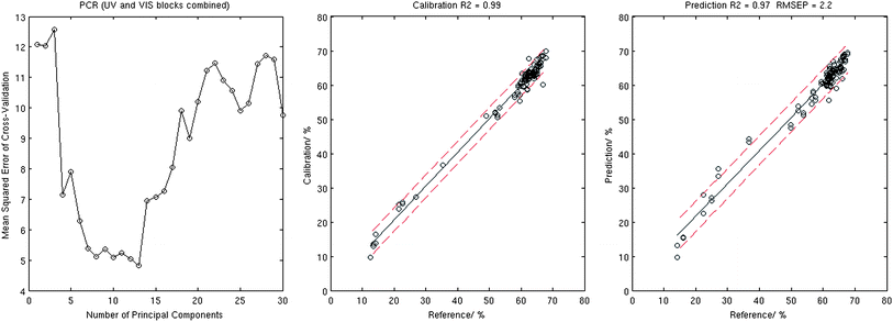Fig. 2 Results of the PCR analysis: MSECV corresponding to the 10-fold cross-validation (left), calibration plot (centre), and validation plot (right).

4.2.2 PLS analysis. The same three data combinations were used in the PLS analysis. Again, the optimal number of latent variables differed significantly between the three cases and was equal to 6 (UV), 11 (VIS), and 6 (UV and VIS combined). As generally expected, PLS provided similar prediction accuracy with a lesser number of latent variables as compared to PCR (see Table 1). The best validation results were R² = 0.97 and RMSEP = 2.2%. In common with the PCR analysis this was achieved using the UV and VIS data combined as the X block. Fig. 3 shows the corresponding MSECV plot for the UV and VIS data as a function of a number of latent variables, as well as calibration and validation plots.

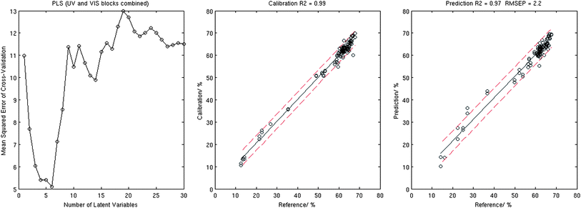Fig. 3 Results of the PLS analysis: MSECV corresponding to the 10-fold cross-validation (left), calibration plot (centre), and validation plot (right).

4.2.3 MB-PLS analysis. A total of 3 latent variables were found to be optimal for the MB-PLS algorithm applied to this dataset. The associated goodness-of-fit parameters for calibration and validation were R²_Cal = 0.96 and R²_Val = 0.94 respectively with RMSEP = 3.1%. The UV and VIS LIBS data were applied as the X₁ and X₂ blocks. Swapping X₁ for X₂ did not have an effect on the outcome of the analysis. This reflects the robustness of the MB-PLS approach. See Fig. 4 for the MSECV, calibration, and prediction plots.

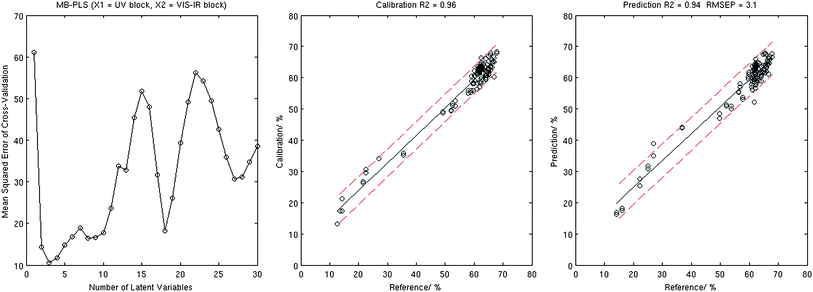Fig. 4 Results of the MB-PLS analysis: MSECV corresponding to the 10-fold cross-validation (left), calibration plot (centre), and validation plot (right).

4.2.4 S-PLS analysis. In contrast to MB-PLS, the S-PLS algorithm is sensitive to the choice of the order of the X blocks used for analysis.¹⁴ Both combinations were considered in the application of S-PLS to the available LIBS data:

1) UV → X₁; VIS → X₂

2) VIS → X₁; UV → X₂

The calibration procedures described in section 4.1 were applied for both cases above acknowledging that the optimal number of latent variables, LV₁, used to decompose X₁ and y is not necessarily equal to the optimal number of latent variables, LV₂, used to decompose X₂ and y.

Indeed the number of latent variables found to be optimal for combination one differed quite significantly for those required for combination two, see Table 1. Taking into account that the UV data block resulted in better performance when used by the standard PLS method, it was somewhat surprising that the X₁ = VIS and X₂ = UV combination demonstrated better prediction results compared to the alternative as the serial nature of the analysis would see the UV X₂ block fine tuning the VIS X₁ PLS outcome. We also note that S-PLS demonstrated much stronger dependency on the number of LVs used for cross-validation computations, which resulted in significantly higher errors achieved for models that used a far from optimal number of LVs. Fig. 5 and Table 1 show that the S-PLS with VIS data in block 1 provides better Fe abundance prediction results with calibration R² = 0.95, validation R² = 0.87, and RMSEP = 4.5%.

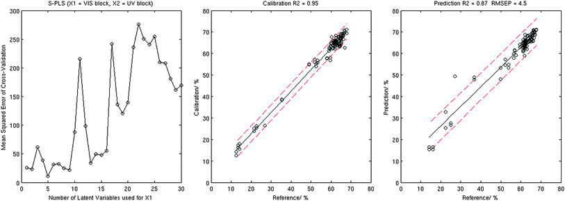Fig. 5 Results of the S-PLS analysis: MSECV corresponding to the 10-fold cross-validation (left), calibration plot (centre), and validation plot (right).

The regression coefficients corresponding to the best performing S-PLS (bottom) and PLS (top) models are demonstrated in Fig. 6. When comparing the two, it is seen that the VIS components have a range of common features, however the values corresponding to the S-PLS case are generally up to a factor of 5 larger. The most noticeable difference is perhaps seen in the UV channel. In contrast to the PLS, for which some of the stronger correlating peaks are located in the UV region, the values of the same coefficients calculated using the S-PLS are relatively small. This difference seems fair considering that these coefficients correspond to the calibration case when the UV spectra were used in a secondary data block. The regression coefficients as such are not used for prediction in the case of the MB-PLS calibration, and therefore not shown in the manuscript. The regression coefficients obtained for the PCR model are very similar to the ones demonstrated in Fig. 6 (top).

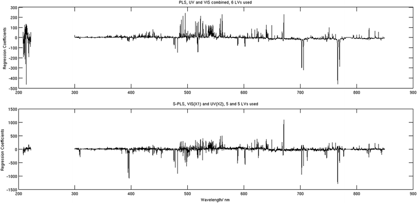Fig. 6 Regression coefficients corresponding to the PLS analysis (top) and to the S-PLS analysis (bottom).

5. Conclusion

PCR, PLS, MB-PLS, and S-PLS algorithms have been applied to and compared for the analysis of Fe in iron ore matrices using laser induced breakdown spectroscopy. To our knowledge, neither MB-PLS nor S-PLS have been used in this way for the quantitative estimation of elemental concentrations from atomic spectroscopy even though they have been used successfully for the analysis of molecular spectra previously.

Two data blocks recorded using the Czerny–Turner and Echelle spectrometers fitted with gated and intensified detectors and covering spectral ranges from 208 nm to 222 nm and 300 nm to 855 nm respectively were analysed. When the combination of UV and VIS data was used for analysis, PCR and PLS provided superior performance for Fe determination with validation R² of 0.97 and RMSEP of 2.2%.

The sole use of the VIS or UV data was found less precise in predicting iron content with validation in the range of R² = 0.90–0.94 and RMSEP in the range of 3.0–3.9% for PCR and PLS. As expected, PLS required significantly less latent variables for calibration compared to PCR.

Results produced by the MB-PLS algorithm which treats the two spectral data blocks separately in a parallel mode were third best, with validation R² = 0.94, and RMSEP = 3.1%. S-PLS algorithm which treats the two data blocks in a serial mode, demonstrated relatively weak performance with validation R² = 0.87 and RMSEP = 4.5%. In both cases these results did not compare favourably with the outcome of the standard PLS and PCR analysis on combined data sets.

The present study shows that in general multivariate data analysis techniques are very well suited for quantitative elemental analysis in iron ore using LIBS spectra. With a range of commercial instruments available for LIBS comprising several compact spectrometers, it seems reasonable to put all available spectral data into a single X block and consider PLS and PCR as first candidates to be used for calibration.

References

1. J. P. Singh and S. N. Thakur, Laser-induced breakdown spectroscopy, Elsevier, Amsterdam, Oxford. 2007.
2. D. A. Cremers and L. J. Radziemski, Handbook of laser-induced breakdown spectroscopy, John Wiley, Chichester. 2006.
3. L. J. Radziemski, Spectrochim. Acta, Part B, 2002, 57, 1109–1113.
4. M. Z. Martin, N. Labbe, T. G. Rials and S. D. Wullschleger, Spectrochim. Acta, Part B, 2005, 60, 1179–1185.
5. N. Labbé, I. M. Swamidoss, N. André, M. Z. Martin, T. M. Young and T. G. Rials, Appl. Opt., 2008, 47, G158–G165.
6. F. C. J. De Lucia, J. L. Gottfried, C. A. Munson and A. W. Miziolek, Appl. Opt., 2008, 47, G112–G121.
7. D. L. Death, A. P. Cunningham and L. J. Pollard, Spectrochim. Acta, Part B, 2008, 63, 763–769.
8. D. L. Death, A. P. Cunningham and L. J. Pollard, Spectrochim. Acta Part B, 2009, 64, 1048–1058.
9. S. M. Clegg, E. Sklute, M. D. Dyar, J. E. Barefield and R. C. Wiens, Spectrochim. Acta, Part B, 2009, 64, 79–88.
10. P. Yaroshchyk, D. L. Death and S. J. Spencer, Appl. Spectrosc., 2010, 64, 1335–1341.
11. B. Jørgensen and Y. Goegebeur, http://statmaster.sdu.dk/courses/ST02/index.html, 2007.
12. P. Geladi, J. Chemom., 1988, 2, 231–246.
13. C. C. Felicio, L. P. Bras, J. A. Lopes, L. Cabrita and J. C. Menezes, Chemom. Intell. Lab. Syst., 2005, 78, 74–80.
14. L. P. Bras, S. A. Bernardino, J. A. Lopes and J. C. Menezes, Chemom. Intell. Lab. Syst., 2005, 75, 91–99.
15. L. E. Wangen and B. R. Kowalski, J. Chemom., 1988, 3, 3–20.
16. J. A. Westerhuis and P. M. J. Coenegracht, J. Chemom., 1997, 11, 379–392.
17. J. A. Westerhuis, T. Kourti and J. F. Macgregor, J. Chemom., 1998, 12, 301–321.
18. A. Berglund and S. Wold, J. Chemom., 1999, 13, 461–471.
19. S. deJong, Chemom. Intell. Lab. Syst., 1993, 18, 251–263.
20. S. W. Chong and I. B. Lee, J. Process Control, 2005, 15, 295–306.

---