The ‘Horwitz ratio’—a study of the ratio between reproducibility and repeatability precisions in the analysis of foodstuffs

Abstract

This paper examines precision statistics from collaborative trials (interlaboratory method performance studies) reported between 1990 and 2000. The principal focus is on the ‘Horwitz ratio’ (s_R/s_r), the ratio of the estimated standard deviations of reproducibility (s_R) and repeatability (s_r) found for individual analytical procedures. A predictable ratio would be a valuable tool in assessing uncertainty and detection limit. While the median ratio observed was close to 2.0, a significant variation with a strong positive skew was observed, much of which could be attributed to particular types of analyte, test material, and analytical procedure.

---

Introduction

The study reported here is concerned mainly with the ‘Horwitz ratio’ s_R/s_r between estimates of standard deviations of reproducibility (s_R) and repeatability (s_r) in analytical procedures. In collaborative trials (interlaboratory method performance studies) in the food sector, it is recognised that the ratio is typically close to 2.0. A mean value of 2.05 was found in a comprehensive survey of the statistics up to 1990 and a value between 1.5 and 2.0 is often assumed by default.¹ In certain legislation² it is assumed that s_R/s_r = 1.5. A comparable relationship may hold in application sectors other than food analysis. Individual values of the ratio among trials must deviate to a degree from the typical value, because both statistics s_R and s_r are random variables based on small numbers of observations and have correspondingly wide confidence intervals. It is also likely that individual trials, each characterising a different analytical procedure (comprising an analyte, matrix, procedure, and measurement principle), have inherently different true ratios, although the existence and causes of this putative systematic effect have not been investigated hitherto.

The magnitude of the ratio, both within and among trials, is an important feature to characterise if it can be predicted reasonably accurately. A broadly constant average ratio would be a useful quantity because it would enable analysts to form a rough estimate of s_R from s_r in instances where information from a collaborative trial was unavailable (a value of s_r can be obtained during single laboratory validation). In turn, a good estimate of s_R is a valuable benchmark that can help analysts to avoid unrealistically small estimates of uncertainty. It is therefore of considerable interest to examine the variability of the Horwitz ratio to see whether it could be used reliably in this context.

The value of a Horwitz ratio may be relevant also to describing the detection capability of an analytical procedure. A detection limit is in effect a small multiple k (2 < k < 4) of the standard deviation of results replicated at or close to zero concentration. But what are the appropriate conditions of replication for estimating this standard deviation? This is a debated issue as a variety of conceivably relevant options are available, in particular instrumental, repeatability, and reproducibility conditions.³ But as reproducibility standard deviation provides the best approximation to uncertainty, the appropriate conditions for characterising detection capability in routine analysis might best be a reproducibility standard deviation estimated at zero concentration.

That statistic would be difficult, often impossible, to obtain directly. In principle, however, it could be estimated by extrapolation to zero concentration of standard deviations estimated at higher concentrations. It is therefore is of interest to determine whether the Horwitz ratios s_R/s_r found in individual collaborative trials is maintained at a constant level down to zero concentration. As repeatability-based detection limits are readily obtained, that information would assist analysts in avoiding unduly low estimates in analytical procedures where no collaborative trial had been conducted. There has been speculation that s_R/s_r → 1 as c → 0, which would greatly simplify matters if found to be true, and that conjecture also needs investigation.

(Note: the ratio s_R/s_r is difficult to determine directly at zero concentration. An authentic test material containing effectively zero concentration of analyte would be nearly always unobtainable. Moreover, organisers of collaborative trials tend to avoid low concentrations of the analyte because of problems in the statistical handling of the results. These problems are an outcome of common data recording practices, namely (a) recording too few significant figures for an adequate statistical analysis and (b) censoring results falling below zero concentration. Sub-zero results have no corresponding physical realisation, of course, but are important in forming unbiased estimates of location and dispersion).

The data

The primary dataset in this study comprised relevant statistics from all collaborative trials in the food sector that were reported between 1990 and 2000. To qualify for the present study, however, the trials had further to comply with the minimal IUPAC recommendation⁴ of eight participant laboratories and five different test materials. After elimination of the non-qualifying studies, the working dataset comprised 782 corresponding values of s_R, s_r, and concentration, derived from 95 collaborative trials relating to food analysis. The median size of the trials in the qualifying subset was 11 laboratories and 6 test materials.

Results and discussion

Variation of reproducibility standard deviation with mass fraction of analyte

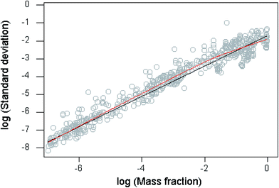
This dataset provides an interesting opportunity to compare moderately recent statistics with Horwitz's databases of collaborative trials dating back to the 1930s, on which the original Horwitz function was based. These were re-examined in detail in 1997 (ref. 1). Then it was found that the trend of the reproducibility statistics followed the Horwitz function closely at mass fractions (c) between 10⁻⁷ and 0.1. A closely similar observation applies over the same concentration range to the statistics in the current study (Fig. 1), where the trend of the data is modelled by a “lowess” function (locally weighted scatterplot smoother—a model-free description of the data⁵). The log-transformed s_R values seemed to be reasonably close to homoscedastic, so an unweighted regression fit was applied to those with mass fractions c falling between 10⁻⁷ and 10⁻¹. The outcome was as follows:

Fig. 1 Reproducibility standard deviation vs. mass fraction above 10⁻⁷, showing the present study data (circles), the original Horwitz function (black line), and a lowess fit (red line). Logarithms are base 10.

• the original Horwitz function; σ_H = 0.02c^0.8495;

• the 1997 study; s_R = 0.0166c^0.824;

• the present investigation: s_R = 0.039c^0.8891.

The recent trend shows a significantly higher s_R than either the original Horwitz function or the 1997 investigation over that part of the range, a trend visible in Fig. 1.

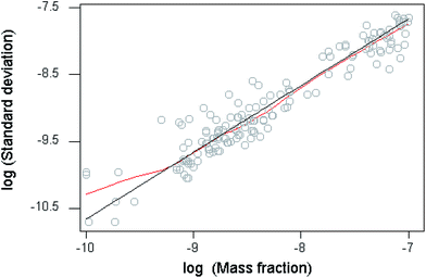
Below a mass fraction of 10⁻⁷ the trend of the precision statistics conforms closely to an underlying constant reproducibility relative standard deviation of 0.22 (Fig. 2), which is consistent with other findings, specifications for fitness for purpose, and constraints imposed by detection capability.⁶ The deviation of the lowess fit from constant relative standard deviation below 10^−9.2 in Fig. 2 is of no consequence given the sparseness of the data.

Fig. 2 Reproducibility standard deviation vs. mass fraction below 10⁻⁷, showing the data from the present study (circles), a constant relative standard deviation of 0.22 (black line), and a lowess fit (red line). Logarithms are base 10.

The Horwitz ratio – summary behaviour

A boxplot of the log-transformed Horwitz ratios (Fig. 3) shows a clearly visible variation among the individual collaborative trials. Log-transformation, as well as making a summary plot possible, serves to stabilise (to some extent) the variance of the ratio among trials. Despite the remaining heteroscedasticity, a one-way analysis of variance (ANOVA) on the whole transformed dataset, that is, between trials and within trials, shows a highly significant between-trial effect with a variance amounting to 40% of the total. This outcome shows immediately that there are real systematic variations among the ratios as well as random, in short, that the mean ratio depends on the particular analytical procedure. While no stronger inference is possible from this ANOVA, the outcome suggests that it would be worth searching for meaningful subsets of trials with overall differing properties, a possibility investigated below.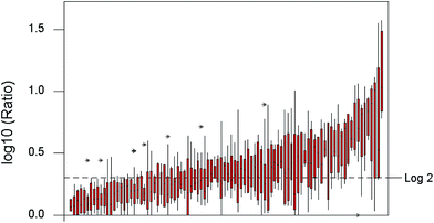

Fig. 3 Boxplot of log₁₀ Horwitz ratios. Boxes show ratios observed within individual trials, arranged in order of increasing mean ratio.

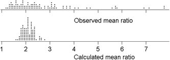
The within-trial mean ratios are summarised in Fig. 4. Some degree of positive skew would be expected, inter alia because the ratio is bounded at 1.0 on the low side, as σ_R ≥ σ_r. The long positive tail on the observed means cannot (as might be thought) be attributed to random deviations. Large simulations, from a model with 11 laboratories, a true ratio of σ_R/σ_r = 2 (bearing in mind that the two standard deviations are not independent), and the random normal assumption of measurement variation, show that the dispersion of s_R/s_r is indeed long tailed on the positive side. However, the distribution of the mean ratios (rather than individual values of the ratio) in median-sized trials, that is with six test materials, was only slightly skewed. Random variation therefore does not account for the observed dispersion of trial means.

Fig. 4 Observed mean ratios from the 95 qualifying trials (some outliers not shown), and 95 simulated mean ratios calculated for an assumed six laboratories under H₀: σ_R/σ_r = 2 and the assumption of the normal distribution of analytical error.

Another worthwhile observation is that the value of the mean ratio within-trial shows no apparent dependence on the mean mass fraction of the analyte (Fig. 5).

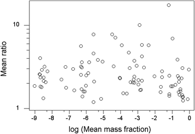Fig. 5 Plot of mean ratios found within trials vs. the mean mass fraction of the analyte. Each point represents a single trial.

Variation of the Horwitz ratio with mass fraction within individual trials

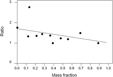
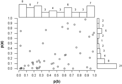
A further possibility is that the Horwitz ratio varies systematically with mass fraction within some individual trials. As a first step, the working dataset was further screened to exclude individual trials that were unsuitable for study by regression analysis. Grounds for this exclusion were as follows: (a) all of the concentrations were in a small range—in such instances regression would be meaningless; and (b) the ratios were very erratic or outlier-prone. From other trials, data from individual test materials were deleted before regression because they would have exerted unduly high leverage on the outcome or because they were obvious outliers as judged by a preliminary robust regression using Theil's complete method.⁷ In any event the regression coefficients were usually strongly correlated, largely because of the relatively large scatter of the dependent variable (that is, the observed ratios). An example dataset is shown in Fig. 6 (Note: the correlation arises because variation in the position of the fitted line affects the slope and intercept simultaneously).

Fig. 6 An example dataset from a single collaborative trial, ‘insoluble dietary fibre’ in animal feeding stuff, showing the Horwitz ratio vs. mass fraction of the analyte and the relationship (line) fitted by regression. Each point represents a different test material.

The outcomes individually were not of great information content because of the (statistically) small number of test materials within each trial. Taken together though, some worthwhile conclusions can be drawn. In the majority of instances (44/50 trials) the slope of the regression line was not significantly different from zero at 95% confidence, that is, there was no suggestion that the Horwitz ratio was linearly dependent on the concentration of the analyte. This outcome hardly differs from an overall null hypothesis (i.e., that there is never a variation with concentration), under which assumption we would on average expect between 47 and 48 instances from 50 trials to be non-significant. This is shown by the near-uniform distribution of the p-values derived from the slope coefficient (Fig. 7). The intercepts show a different pattern, with 16 instances (32%) significantly different from 2.0 (Note: strictly speaking, in instances like these, where there tends to be a strong correlation between the estimated regression coefficients, we should consider their joint confidence region rather than the individual confidence limits. Fig. 8 shows the example previously-used in Fig. 6, where the null hypotheses (β = 0, α = 2) fall within the individual 95% confidence limits of the estimates (b, a) but outside the 95% joint confidence region. This refinement would not affect the broad conclusions in this study).

Fig. 7 Marginal histogram plot of the probabilities (p(a), p(b)) associated with the estimates of intercept (a) and slope (b) of the regression line of ratio vs. concentration, in relation to the null hypotheses β = 0, α = 2. In the general absence of effects, independent random uniform distributions U(0,1) would be expected.

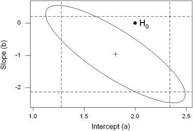Fig. 8 Strongly correlated regression coefficients (cross) showing the null hypotheses H₀: β = 0, α = 2 (solid circle), which in this instance falls outside the joint 95% confidence boundary (ellipse) of the coefficients but inside their individual 95% confidence limits (dashed lines). Same data as Fig. 6.

Among the 50 trials included in this part of the study, there was no suggestion of the ratios changing radically at concentrations approaching zero.

Dependence of the ratio on analyte type

Given that the distribution of intercepts shows a mode close to 2.0 but a strong positive skew, it is of interest to find whether the value depends on the analyte type, the test material type, or the physical principle on which the measurement procedure is based. Fig. 9 shows variation among the mean Horwitz ratios, each from a separate trial, classified by analyte type. It is clear that the majority of the types give ratios located near 2.0, but two types, trace elements and individual fatty acids, have much higher tendencies and account for the positive skew.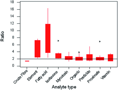

Fig. 9 Boxplot of mean Horwitz ratios from all 95 trials, classified by the type of analyte. The width of the boxes is proportional to the number of collaborative trials in each class.

It is interesting to consider the origin of these anomalously high ratios, which could result from either exceptionally low s_r or unusually high s_R. The former would be expected of a simple procedure involving say only a few high-precision measurements and no complex chemistry or skilful manipulations (loss on drying would be an example). The latter would be expected when environmental or organisational factors affecting the results might differ substantially between laboratories. In the present study we see both circumstances in play, as shown below in the following average values of the standard deviations for the two anomalous subsets relative to those of the other types.

Analyte type	s r	s R
Oil/fat	0.45	1.16
Element	0.78	1.44

Both analyte types show a lower-than-typical s_r, and a higher-than-typical s_R. In the former instance, as s_R is only slightly above average, no great problem exists for the quality of analysis, despite the high Horwitz ratio. For trace elements, however, the elevated value of s_R suggests that an investigation of the causes might lead to a useful improvement of quality in that area. In this instance the high values of s_R have been found often to be caused by contamination or variable recovery, while the within-laboratory variation is small because the procedures are largely instrumental. However, the reverse effect is noted when considering methods of analysis for crude fibre. Here the procedure is usually very manipulation-dependent so the within-laboratory results tend not to be very consistent. If the value of s_r is equal to s_R, as can occasionally happen by chance, then the ratio is set conventionally to unity. This is most likely to occur when very manipulation-dependent procedures are being considered.

This particular classification by analyte type correlates strongly with classification based on test material type and type of analytical method, as the fatty acids were determined exclusively in oily test materials by gas chromatography, but the individual elements were determined largely by atomic spectrometric methods after destruction of the organic matrix. In short, there is no further information to be gained by alternative classifications of the ratios by matrix or physical principles of analysis.

Conclusions

The following have been established in relation to the Horwitz ratio in the food analysis sector.

• In the great majority of procedures the ratio does not change significantly with the concentration of the analyte. In particular there was no evidence that the ratio changed abruptly at concentrations near zero, so that mean values (robustified if necessary) within a trial were valid estimates of the zero-point ratio in most instances. When, in the small proportion of instances, significant dependence between the ratio and concentration was observed, regression intercepts would be alternative valid estimates of the zero-point ratio.

• There was no evidence to support the idea that the ratio tended towards unity at concentrations near zero.

• The mode of the ratios was close to 2.0. The strong positive skew in the observed mean ratios was apparently due to special circumstances prevailing in specific types of analysis. In a majority of individual trials the mean ratio observed was not greatly different from 2.0. An assumption of a value of 2.0 for the purpose of gauging the value of s_R from s_r would be safe in most instances in food analysis, but not in the determination of trace elements or constituents of oils and fats.

• Whether the assumption of a ratio close to 2.0 would be valid in application sectors other than food is unknown, as the relevant statistics (that is, obtained from collaborative trials of specific procedures) are not currently produced in sufficient numbers to allow generalisation. Proficiency test statistics mostly cannot be considered as alternatives as they do not characterise procedures but the performance of participants free to use any measurement principle or procedure.

References

1. M. Thompson and P. J. Lowthian, J. AOAC Int., 1997, 80, 676–679.
2. Commission regulation (EC) no. 333/2007, Laying down the methods of sampling and analysis for the official control of the levels of lead, cadmium, mercury, inorganic tin, 3-MCPD and benzo(a)pyrene in foodstuffs OJ L88/29 of 29.3.2007.
3. M. Thompson, Anal. Methods, 2012, 4, 1598–1611.
4. W. Horwitz, Pure Appl. Chem., 1995, 67, 331–343.
5. W. S. Cleveland, J. Am. Stat. Assoc., 1979, 74, 829–836.
6. M. Thompson, Anal. Methods, 2013, 5, 4518–4519.
7. W. Bablok and H. Passing, J. Autom. Chem., 1985, 7, 74–79.

---