Sampling theory and sampling uncertainty
Analytical Methods Committee, AMCTB No. 71
First published on 24th November 2015
Abstract
We make a chemical measurement mostly to help make a rational decision about a ‘target’, a particular mass of material that is of interest in manufacturing, commerce, human health, or for cultural purposes. A target might comprise for example a shipment of a raw material, a batch of a manufactured product, the topsoil in a brown-field site, or a patient's blood. Chemical analysis, like all measurement, gives rise to an inevitable degree of uncertainty in the result. But you can seldom analyse a whole target—you have to work on a sample—and sampling introduces its own uncertainty. All of this uncertainty should be taken into account in decision making.
Samples, however carefully taken, always differ in composition from the target mean: randomly replicated samples from the same target always differ among themselves. These deviations determine the sampling uncertainty. To make a rational decision, then, this uncertainty derived from sampling has to be combined with that arising from analysis. After all, the customer needs to make a decision about the target, rather than about the sample, although this distinction is often overlooked. It is the combined uncertainty that helps make those rational decisions. One of the first things that we need to know is that this uncertainty is good enough, that is, fit for purpose.
Uncertainty of measurement arising from sampling (UfS) is usually non-negligible, especially so with raw materials and environmental materials where indeed UfS often exceeds the analytical contribution. So how should we cope with the uncertainty from sampling? There are two different schools of thought about that.
The ‘theory-of-sampling’ (TS) school of thought
The theory of sampling (TS) is a detailed itemisation of the mechanical structure and chemical variation within a target in relation to the procedure for obtaining a primary sample from it. Features of the target that are considered include the size range of the particles comprising the target, the shapes of the particles, the compositional variation of the particles and the degree and style of the heterogeneity of the target. Important features of the procedure are the method of extracting the primary sample, its mass, and its degree of comminution at various stages of the sampling operation. This detailed study identifies about ten separate types of ‘error’. (Note: the TS is not at present framed in VIM3-compliant terminology.) These ‘errors’ generally have to be eliminated, and that attention to detail defines a procedure (the sampling protocol) that delivers a sample regarded as ‘correct’.The intended interpretation of ‘correct’ is ‘unbiased’ so sampling bias (admittedly a tricky topic) is obviated by definition. This is a potential weakness in TS—anybody having a practical acquaintance with sampling will be well aware of sources of bias. An obvious example is sampler bias, how an individual sampler executes the protocol. Perhaps more importantly, an attribute sometimes incorrectly ascribed to a ‘correct’ sample is that any residual UfS makes a negligible contribution to the combined uncertainty. In short, the application of TS may be mistakenly taken to imply that you can ignore sampling uncertainty and take into account just the analytical uncertainty.
Strengths and limitations of the ‘theory-of-sampling’ approach
In reality TS is often poor at predicting UfS quantitatively, because the modelling required for a good prediction would be far too complicated and mathematically intractable. So a UfS estimated from a TS model would need to be validated experimentally before the sampling protocol could legitimately be accepted as appropriate. A further problem needs to be considered. Successive targets, especially of unprocessed materials, differ from each other in numerous ways, so a protocol that delivers a suitable sample from one target may do otherwise for the next one ostensibly of the same kind.It is difficult, however, to fault the TS as a qualitative method of arriving at what is prima facie a reasonable procedure, except perhaps on the grounds of the effort required. Much of the theory is commonsensical and, moreover, the process will be educational for trainee samplers. However, the sampling procedure thus arrived at will need validation (and possibly some amendment) before it can be accepted as fit for purpose. This is because it is difficult indeed and often very laborious to quantify many of the ‘errors’ (not to mention their interactions, which are usually ignored), so the ‘correctness’ cannot be taken for granted. Furthermore the aim of TS is less to make an explicit estimate of the uncertainty arising from the sampling than to provide a ‘representative’ sample that can be sent to a laboratory without contributing any apparent uncertainty.
The experimental school of thought
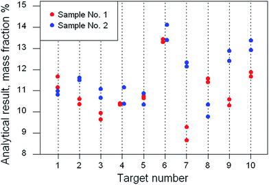
The alternative school of thought holds that, in a properly randomised experiment, simply replicating the application of any sampling protocol gives a useful estimate of the uncertainty of the resultant measurements arising from sampling. (That is why the strategy is sometimes confusingly called the ‘Measurement Uncertainty’ (MU) approach.) The protocol under test could be arrived at by any means: by tradition, by an evolutionary process, from TS, or simply by judgement based on experience. If properly conducted, the replication can encompass much of the potential uncertainty and lets us judge whether the protocol is fit for purpose. (The designs shown below, however, cannot incorporate uncertainty relating to operator/method bias.)A parsimonious experimental approach is to make randomised duplication a part of routine sampling (by using a provisional protocol) until the required amount of data is obtained. This ensures that the uncertainty estimate obtained represents real-life conditions rather than an artificial experimental situation. The design shown in Fig. 1 (or an even more economical unbalanced version) is appropriate. Results are collected until there are enough to allow a reasonably stable estimate of the between-sample variance by hierarchical ANOVA (analysis of variance). (After that, the occasional duplicate sampling of a target can be regarded as merging into internal quality control of sampling.) A set of results from such a test might resemble those depicted in Fig. 2.
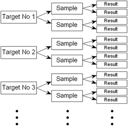 | ||
| Fig. 1 Design of a balanced duplicated sampling experiment. An unbalanced design reduces the analytical burden by 25% (see AMCTB no. 64). | ||
A careful visual examination of the data is an essential preliminary step, to ensure that a suitable statistical approach is employed. In Fig. 2 we see successive targets of similar composition apart from one possibly anomalous target (no. 6). However, a single anomalous target per se will not affect the nested ANOVA because the between-target dispersion is not relevant here. Between-sample variation is apparently greater than analytical variation. There is no suggestion of heteroscedasticity or that the first sample differs systemically from the second. Target no. 7 has the biggest difference between samples but it is not clear visually that the difference is outlying. Either way, a robust ANOVA can cope with this dataset, providing an estimate for the ‘typical’ value of the between-sample standard deviation. The statistics obtained were: grand mean, 11.1% mass fraction, between-target SD, 0.15; within-target/between-sample SD, 1.01; analytical (within-sample) SD 0.32.
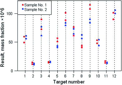
In instances where the results are heteroscedastic (that is, the analytical and/or sampling standard deviation varies with the concentration of the analyte) a more complex type of statistical analysis may be required. Fig. 3 shows such a dataset. It is evident there that the dispersion of both analytical and sample duplicates is greater at high than at low concentrations. A suitable treatment for this particular dataset might be log-transformation before ANOVA is attempted. That would tend to stabilise the variance, a requirement for a usable outcome of ANOVA. An examination of the residuals would show whether that strategy had been successful.
Limitations of the experimental approach
A clear shortcoming of replication is that, in the event of the protocol being rejected as being unfit for purpose, we have no immediate diagnostic information to locate and rectify the source of the problem. Further experiments would be required. In addition, we have already seen that the duplicate method fails to incorporate sampler bias and method bias, and for the present time we have perforce to accept that circumstance. It is not even clear whether these factors generate uncertainty of noteworthy size, except in the few instances that have been studied to date. A sampling analogue of the analytical proficiency test would be required to include those contributions, and such tests are not yet generally available. We must also note that the duplicate method provides an estimate of repeatability analytical standard deviation: a credible estimate of analytical uncertainty therefore has to be derived by other means.Afterthoughts
•The best that we can expect from a replication experiment on a succession of targets is an indication of a typical between-sample uncertainty. There is no guarantee that the next target won't be atypical in some way, perhaps more heterogeneous. Because of this, it is in principle possible that a sample obtained via a fit-for-purpose protocol may not itself be fit for purpose. Only diligence on the part of the sampler and internal quality control of sampling could help to guard against that.•The phrase ‘representative sample’ has been used by analytical chemists with a variety of nuances but mostly in an implicitly qualitative context. Perhaps, given this, we should replace the word ‘representative’ with a phrase like ‘optimally useful’. If ‘representative’ seems indispensable, however, it should be normatively defined in terms of ‘a suitably small uncertainty from sampling’.
Further reading
•Eurachem/CITAC Guide: Measurement uncertainty arising from sampling: a guide to methods and approaches.•K. H. Esbensen and C. Wagner, TrAC, Trends Anal. Chem., 2014, 57, 93–106.
•AMC Technical Briefs, no. 16A, 19, 31, 32, 42, 51, 58, 60, 64.
This Technical Brief was drafted by the Uncertainty from Sampling Subcommittee and approved by the Analytical Methods Committee on 13/11/15
.
| This journal is © The Royal Society of Chemistry 2015 |

