Black-box determination of temperature-dependent susceptibilities for crystalline organic radicals with complex magnetic topologies

Abstract

In all but the simplest crystal structures, the identification of all relevant interactions between magnetic sites as well as the setup of magnetic model spaces, which are necessary for modeling macroscopic magnetism, are tedious and error-prone tasks. Here, we present a procedure to generate magnetic susceptibility versus temperature curves using only a crystal structure as input. The procedure, which is based on the first-principles bottom-up approach [Deumal et al., J. Phys. Chem. A, 2002, 106, 1299], is designed in a way to require as little user interference as possible. We employ quantum chemical calculations to parametrize a Heisenberg Hamiltonian, which is set up and diagonalized for different magnetic model spaces to ensure convergence of the model. We apply the procedure to several 6-oxo-verdazyl radical structures, including newly synthesized compounds, and compare the results to data we obtained from magnetic susceptibility measurements as well as published data to further benchmark our procedure. Furthermore, the different impact of certain dominating coupling constants is systematically analyzed.

---

1 Introduction

Predicting the magnetic behavior of a substance directly from ab initio calculations is a tough challenge for quantum chemistry. Single molecule parameters like hyperfine coupling constants, which are relevant for the interpretation of electron paramagnetic resonance (EPR) experiments, can be obtained with a decent accuracy from wavefunction and hybrid density functional theory (DFT) calculations.¹ However, at least DFT methods are not able to reproduce highly accurate data for a direct prediction of a spectrum.

The situation is much worse for the prediction of the magnetic susceptibility, which stems from interactions between different magnetic units. This bulk property is sensitive to the packing of the substance in a crystal structure. Thus, quantum chemical calculations can only be performed for substances for which accurate crystal structures are available.

If all spin states are known, the magnetic susceptibility can be calculated from a Boltzmann distribution as a temperature-dependent quantity,²

where N is the Avogadro constant, g the gyromagnetic constant of an electron, μ_B is the Bohr magneton, k_B is the Boltzmann constant, μ₀ is the vacuum permeability, and the sum is taken over all spin states n, each of which is described by its spin S_n and energy E_n. S₀ and E₀ indicate the values for the ground state.

However, the number of possible spin states in a periodic structure is infinite. In their first-principles bottom-up approach Deumal et al.³ use a finite system to model the properties of the structure. According to their approach, one first needs to identify all relevant magnetic interactions and calculate the corresponding magnetic exchange coupling constants. With the gained information a magnetic motif can be identified, which can have a dimensionality of 0D (e.g. isolated dimers), 1D (e.g. spin chains or spin ladders), 2D (e.g. a net structure) or 3D (a network). Next, a so-called minimal magnetic model is set up which contains all information needed to represent the magnetic motif using as few magnetic sites as possible, where a magnetic site is a spin-bearing unit to which a local spin can be assigned. In the case of an organic radical structure a magnetic site typically corresponds to one molecule. The magnetic model can be represented by its Heisenberg Hamiltonian,

Here, the J_AB are the magnetic exchange coupling constants and Ŝ_X is the spin operator for a local spin on site X. In its matrix representation the Hamiltonian can be diagonalized to yield the spin states needed to solve eqn (1). Note that the Hamiltonian assumes isotropic, pairwise interactions only. To conclude the computational procedure, the magnetic model is extended until convergence is reached.

With this strategy the problem to solve with a quantum chemical method is reduced to the calculation of the magnetic exchange coupling constants J. For reviews concerning the parametrization of Heisenberg Hamiltonians see ref. 4 (with a focus on DFT calculations) and ref. 5 (with a focus on wavefunction methods). The coupling constants can be obtained from the energy differences of the different spin states of each unique pair of spin centers or magnetic sites. According to the Landé interval rule⁶ or with a spin–flip time-dependent DFT (SF-TD-DFT) approach^7–9 the calculation of a state with maximum spin and one low-spin state is sufficient.^10,11 While the maximum-spin state can be described qualitatively correctly with a single Slater determinant, this is not true for the relevant low-spin states. These low-spin states in a pair of magnetic units are open-shell states for which standard single-determinant methods like Hartree–Fock (HF) and DFT cannot be reliably applied. For small systems correlated wavefunction methods may yield excellent results, but they are too expensive for large systems. In these cases, methods like SF-TD-DFT or the broken symmetry (BS) approach¹² are typically used, although they are known to yield results which are usually not in quantitative agreement with experimental data. As is inherent to all single-determinant methods, these methods may lead to wrong results if static correlation is important beyond the magnetic orbitals, which can also be the case in organic systems.¹³

The approach to obtain spin states and magnetic susceptibilities by quantum chemical parametrization and diagonalization of the Heisenberg Hamiltonian is well-established.^2,13–17 At the same time, it can be observed that the majority of studies in this field still does not employ the complete first-principles bottom-up approach as introduced in ref. 3. In fact, many studies are restricted to the calculation of pairwise magnetic exchange coupling constants.^18,19 Other investigations use simplified expressions for the magnetic susceptibility and obtain coupling constants and susceptibility curves by fitting to experimental data.^20,21 Such fitting strategies need to be applied with caution. If a system cannot be described correctly with a simple model including a small number of fitted parameters, the results can quickly become ambiguous.⁴ As we will point out, a reason for this limited use of the first-principles bottom-up approach may be due to the difficulties in some of the crucial steps in the procedure, which require expertise and a lot of manual work. A reliable and simple software tool for automatizing these critical steps would thus be highly appreciated.

Despite the small number of families of persistent organic radicals, many magnetically active compounds have been realized so far. Here, we only want to point the reader to a few reviews in ref. 22–26. One class of stable radicals, which is getting increasing attention, is the family of verdazyl radicals.^21,27,28 They are common magnetic building blocks and are thus often used to create metal-free or hybrid metal–organic materials with magnetic properties.^22,23 The main reason for the stability of verdazyl radicals is the delocalization of the unpaired electron over the verdazyl ring itself, which is often further extended to aromatic substituents. Packed into a molecular structure many small magnetic interactions are thus possible between the molecules. As a result, a quite complex magnetic model space is needed to properly represent all relevant interactions between the molecules. The same situation can be expected also for other magnetically active molecular compounds.

Especially for such organic radicals with a complex packing of the molecules the identification of all relevant interaction pairs while respecting symmetry (to avoid multiple calculations of the same coupling) is a thankless task to be done manually. The same is true for the correct identification of the magnetic motif and the setup of the corresponding minimal magnetic model. As will be shown in Section 2.3.1, sticking with the crystallographic unit cell can lead to erroneous results.

Here, we present a procedure which wraps up the whole first-principles bottom-up approach to easily get from a crystal structure to a plot of a magnetic susceptibility vs. temperature curve. We automatized the identification of symmetry-unique pairs of magnetic units (see Section 2.1) and avoid the need for a manual interpretation of the coupling constants. Thus, instead of a user-specified magnetic motif, we construct a magnetic unit cell based on an internal set of rules defined in Section 2.3. This turns the magnetic motif from an input parameter into a result. In combination with a reliable quantum chemical method for the calculation of the exchange coupling constants and assistance in convergence checks and interpretation of the results, we provide a methodology which can be easily used by non-experts in the field and enable the first-principles bottom-up approach as a routine method to be carried out alongside with measurements of the magnetic susceptibility in complex organic radicals.

We apply the procedure to a variety of novel 6-oxo-verdazyl radical systems shown in Fig. 1. We reinvestigate molecule 1, for which magnetic susceptibility data is available in the literature,²¹ in order to benchmark our method. At the same time we provide detailed microscopic information based on quantum chemical calculations to back up the results which were obtained by fitting only in the original publication. As an additional literature example, we show results obtained with our approach for a thiooxo-verdazyl adduct²⁹ in the ESI.† Additionally, we analyze in detail the magnetic structures of molecules 2 to 5 which were synthesized and characterized in our collaborative research center. Ferromagnetic interactions in those kinds of verdazyl radicals are very uncommon. In order to achieve a ferromagnetic network similar to the situation in compound 1, we replaced the N-methyl with an N-phenyl-group in compound 5. The precursor compound, a TMS acetylene substituted radical 4, was also investigated in detail.

Fig. 1 The 6-oxo-verdazyl radicals investigated in this study: 1,5-dimethyl-3-(4-ethinyl)phenyl-6-oxo-verdazyl radical (1),²¹ 1,5-diphenyl-3-(anthracene-9-yl)-6-oxo-verdazyl radical (2),²⁸ 1,5-diphenyl-3-(4-(diphenylamino)phenyl)-6-oxo-verdazyl radical (3), 1,5-diphenyl-3-(4-(trimethylsilyl)ethinyl)phenyl-6-oxo-verdazyl radical (4), and 1,5-diphenyl-3-(4-ethinyl)phenyl-6-oxo-verdazyl radical (5).

2 Computational procedure

The input for the procedure is a sufficiently large cutout from the crystal structure (e.g. 3 by 3 by 3 unit cells, where all fragments should be completed) and the six lattice parameters, the lengths a, b, c of the cell vectors and the angles α, β, γ between them. The main part of the procedure is completely automatized and summarized here:

• The individual molecules are identified and it is tested whether they are inside the central unit cell

• Based on the smallest interatomic distance for every pair of molecules, possible interactions are identified

• Symmetry relations between the molecules and interactions are identified

• A symmetry-unique set of pairs is chosen and a mapping to other possible interactions is established

• Structure files for the radical pairs, for which non-negligible magnetic interactions are expected, and input files for BS calculations are written

• The results of the BS calculations are parsed to find extended (periodic) chains of relevant interactions, which can be responsible for macroscopic magnetic behavior

• Possible basis vectors for the magnetic unit cell are identified and an ideal set of such vectors is chosen (see Section 2.3)

• Magnetic models of different sizes are set up

• The Heisenberg Hamiltonian is set up and diagonalized for the different magnetic models

• The results are checked for convergence with respect to the size of the magnetic models

Several of the above points need a more detailed explanation given in the following. Further details are also given in the ESI.†

2.1 Identification of interacting pairs

Magnetic interactions are known to decay rapidly through space.³⁰ Thus, a distance-based criterion can safely be applied for the identification of possible interactions between the sites. We chose as a criterion the smallest distance between any two atoms of two molecules. If any interatomic distance is below a threshold of 4 Å, which is well above twice the van der Waals radii of the atoms of the first two periods,³¹ a possible interaction is taken into account. While this strategy is simple and robust, an experienced user still may exclude certain pairs, e.g. if the radical-bearing groups are far away from each other. However, especially in verdazyl radicals the unpaired electron is typically further delocalized over aromatic substituents at the nitrogen atoms. To be on the safe side it is advisable to skip such a manual preselection, having in mind that BS-DFT calculations are comparatively cheap.

To find all interactions within a unit cell without double counting any interactions, two cases need to be considered. An interaction belongs to the unit cell if either both interaction partners or just one interaction partner is inside the unit cell. In the latter case the interaction partner outside the unit cell has a translational equivalent inside the unit cell which must interact with a translational equivalent of the interaction partner inside the unit cell. These corresponding interactions must be identified and filtered to avoid double counting.

2.2 Broken symmetry calculations

Based on preliminary tests we chose the following setup for the quantum chemical calculations: ORCA³² was used for BS calculations with the PBE0 hybrid functional³³ and a minimally augmented polarized triple zeta basis set (ma-def2-TZVP).³⁴ Very tight convergence criteria were employed (10⁻⁹ Hartree energy difference, keyword “VERYTIGHTSCF”) and no density fitting³⁵ was used. This protocol can of course be easily exchanged by any other method which yields reliable pairwise magnetic exchange coupling constants.

2.3 Creation of a magnetic unit cell

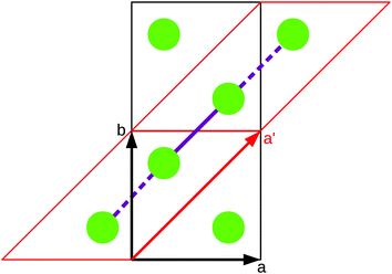
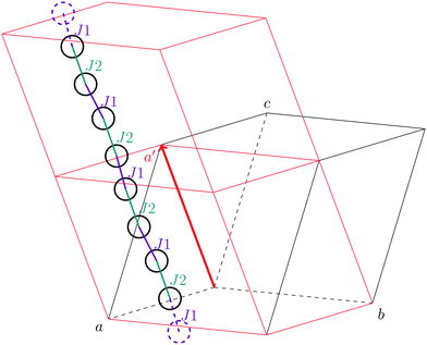
As stated in the original work by Deumal et al., the magnetic unit cell (corresponding to a certain magnetic motif) may be very different from the crystallographic cell (nuclear structure).³ Thus, finding an ideal magnetic unit cell in an automated fashion is a key aspect of this work. We will describe our strategy in detail in this section. However, before giving details about our implementation we will illustrate with a simple model example how severe the impact of a bad choice for the magnetic unit cell can be.

2.3.1 Relevance of a well-chosen magnetic unit cell. Let us assume a linear magnetic chain which contains, for the sake of simplicity, a single repetitive ferromagnetic coupling. Let us assume further that the interaction chain is oriented into the direction of one of the diagonals or the space diagonal of the crystal structure as depicted in Fig. 2. A situation similar to this model is present for molecule 4, if the weak interchain interaction is neglected. That particular system, which contains alternating ferromagnetic and antiferromagnetic couplings, is further discussed alongside with the results for the other substances in Section 4.4.

Fig. 2 A sample system consisting of two magnetic sites (green) coupled to a chain. The interaction chain (purple) passes through the ab diagonal of the unit cell (black). A differently shaped magnetic unit cell (red) with the cell vector a′ is a much better choice to set up magnetic models.

To obtain converged macroscopic data we have to increase the magnetic model starting from an isolated dimer until convergence is reached. Without choosing a proper magnetic cell one may be tempted to increase the model into the directions of the unit cell. Doing this, however, does not primarily increase the length of the interaction chain, but instead it increases the number of isolated dimers in the model. To obtain converged results for the model system shown in Fig. 2 with this strategy, the model has to be increased at least into two of the three axes (a and b directions) at the same time; if the interaction goes through the space diagonal of the unit cell even a simultaneous extention into all three directions is needed. In this way, the model size needed to arrive at converged results can quickly become much larger than what is treatable in terms of computational time and memory requirements. Consider for example a system with two magnetic sites inside one unit cell. Then, a magnetic model of 2 by 2 by 2 cells leads to a Hamiltonian matrix of dimension 2¹⁶ by 2¹⁶, which is close to the limit of what computers can handle nowadays. A model of 3 by 3 by 3 cells already leads to a matrix of dimension 2⁵⁴ by 2⁵⁴. Such a matrix could not even be stored if all the hard drive capacity in the world would be used.

Even worse, if the model is not increased in the correct fashion, the results may seem to be converged immediately as shown by the red, solid curve in Fig. 3. Clearly, this is because there are no interactions between the dimers. In fact, instead of a magnetic chain (1D) one obtains results for a system of isolated dimers (0D).

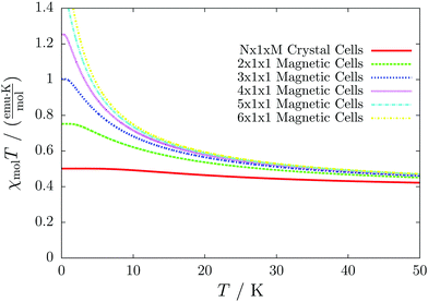Fig. 3 The temperature-dependent magnetic susceptibility, plotted as susceptibility times temperature, for different magnetic models of the model system shown in Fig. 2. The red, solid line is obtained from inappropriate models like the one containing only one unit cell or any model which is not extending the model along the direction a′.

If the model is instead enlarged along the space diagonal one can monitor convergence towards a clearly ferromagnetic system (see the other curves in Fig. 3).

2.3.2 Identification of periodic interaction chains. It is clear that any useful definition of a magnetic unit cell must be based on the magnetic interactions inside the system. Often, different interactions have to be combined to form interaction chains to leave the regime of isolated interactions. In the following we will use the term interaction chain equivalently to a vector connecting the magnetic sites at the beginning and the end of such chains.

To come up with a set of rules to determine the axes of an ideal magnetic unit cell we need to be clear about some properties of the cell and the magnetic interactions within. Although the unit cell and a well-chosen magnetic unit cell may be very different, they clearly share the same periodicity in certain regards. E.g., the volume of the magnetic unit cell must be an integral factor of the volume of the unit cell. (In special cases, however, all magnetic information of a system may already be present in a fraction of a unit cell. We describe our treatment of this case in the ESI.† An example will be discussed in the context of molecule 4 in Section 4.4.) Furthermore, an interaction chain cannot be periodic if it does not pass through the whole unit cell. If an interaction chain is not periodic, it is no candidate to indicate an axis of the magnetic unit cell. Note that this does not at all determine whether an interaction chain is relevant and whether it must be respected in the magnetic model. Another condition for an interaction chain to be periodic is that a translational equivalent of the magnetic site at which the interaction chain starts must be reached. In an equivalent formulation the former condition can be easily included, leading to the following condition for an interaction chain to become a candidate to form one of the axes of the magnetic unit cell:

An interaction chain can represent an axis of the magnetic unit cell if it passes through the unit cell an integral amount of times (including zero) into each direction and at least once into one of the directions.

2.3.3 Dimensionality of the magnetic system. If all periodic interaction chains have been found, the dimensionality of the magnetic interactions in the system is directly available. It equals the number of linearly independent periodic interaction chain vectors, which can naturally only be a number between zero and three. If there are less than three linearly independent directions the original unit cell vectors are used to form the other dimensions of the magnetic unit cell. In that case the magnetic models are never extended into these additional directions.

2.3.4 Ranking the interaction chains. Once a set of axes for the magnetic unit cell is determined an extension of the magnetic model along these axes is straightforward. However, often there are many linearly dependent periodic interaction chains among which a set of axes must be chosen. In principle, convergence has to be ensured into the directions of all periodic interaction chains at the same time. In practice, this is however not possible for most systems due to the exponential growth of computational effort with respect to the size of the magnetic model. Our strategy to solve this problem is to choose the axes for the magnetic unit cell by the expected relevance of interaction chains for the convergence of the magnetic model. Then, we separately test the model for convergence into these directions (see also Section 2.6).

Certainly, the strengths of the magnetic interactions, i.e. the absolute value of the magnetic exchange coupling constants J, must be considered for ranking the interaction chains. If a chain contains interactions with different strengths we only consider the weakest interaction in the chain. The reasoning is that in the limit of a vanishing coupling inside a chain the chain itself will not be periodic any more so that convergence does not have to be checked into that direction. Among chains with the same weakest coupling strength we prioritize shorter chains in terms of the number of couplings in the chain.

Although these rules still do not always lead to a unique solution we did not introduce additional rules because we consider all possible results of this procedure equally reasonable. Starting from the top of this list we use the first three linearly independent interaction chains as the cell vectors of the magnetic unit cell.

2.4 Construction of magnetic models

Our procedure does not require a user-defined magnetic motif as input. The magnetic models are constructed directly from the magnetic unit cell. In fact, the magnetic motif is resembled in the magnetic unit cell and its dimensionality. Thus, we use the magnetic unit cell as the minimal magnetic model. As it has been stated before, we construct larger magnetic models by repeating this cell into the direction of the cell vectors of the magnetic unit cell. There are, however, two possibilities to treat the boundary of the magnetic model. Either, the ends of the interaction chains are left open (corresponding to a finite approximation to the infinite structure), or, as the systems are periodic, interactions may be continued to the opposing side of the magnetic model, forming closed rings of interactions. As it has been shown in ref. 3, the results of both strategies are similar.

In an open model the results are in principle dependent on the choice of the origin of the magnetic model. Instead of working out a strategy to find an ideal origin and to test the effects of different choices, we chose to construct ring models only in order to avoid further complications.

2.5 Setup and solution of the Heisenberg Hamiltonian

Given a magnetic model and the coupling constants which represent the interaction between the magnetic sites in the model it is straightforward to calculate the elements of the Heisenberg Hamiltonian matrix. We currently perform a full diagonalization of the Hamiltonian matrix. This severely limits the number of magnetic sites which can be treated inside the magnetic model, because the dimension of the matrix is 2^N, where N is the number of magnetic sites in the model. Due to the rapid convergence of the data with increasing size of the magnetic model space this limitation is often not a problem in practice. In cases where no convergence is reached yet with feasible sizes of the magnetic models, one could make use of the sparsity of the Hamiltonian matrix. If one is only interested in the lowest energy states, Krylov subspace methods like the Davidson diagonalization³⁶ or a Lanczos algorithm³⁷ can be employed (see ref. 38 for an application to a Heisenberg Hamiltonian). However, the direct application of such methods is not sufficient to calculate temperature-dependent data, because the full eigenvalue spectrum is required for a reasonable Boltzmann distribution in the whole temperature range. If only the energetically lowest spin states are included in the calculation of the magnetic susceptibility, the error increases significantly with increasing temperature. In such cases the high temperature regions can be modeled much better by using Monte Carlo simulations.³⁹

2.6 Convergence check

Once a magnetic unit cell has been defined a magnetic model can be easily extended to check for convergence of the results. Although finally the results must be critically checked by the user and additional convergence checks might become necessary, we came up with a standard protocol which reasonably deals with this issue in many cases. Even if no full convergence is reached in this way, an excellent starting point is provided for additional manual convergence checks.

A user-defined parameter limits the number of allowed magnetic sites in the magnetic models. Our program then produces all possible magnetic models which do not exceed this number of magnetic sites by repeating the magnetic unit cell into all of the up to three axes of the magnetic unit cell which need to be checked for convergence. Extentions into different directions at the same time are also considered. For each of the magnetic models constructed in this way also a picture is generated which includes the magnetic model, the magnetic and the nuclear unit cell and all magnetic sites and interactions of the (sub)system. Several of these models are chosen as suitable candidates for a convergence check by a procedure described in detail in the ESI.† In that context also a reference model is chosen to which other (smaller) models are compared.

For each of the considered models the temperature-dependent magnetic susceptibility is calculated by solving the Heisenberg Hamiltonian and applying eqn (1). Finally, the average mean relative deviation of the different curves is calculated by

where χ₁(T) and χ₂(T) are the curves to compare, sampled at n different temperatures T ∈ [0 K, 300 K]. Of course, more advanced error criteria could be considered, which emphasize the importance of certain temperature regions by an additional weighting factor. We found, however, that our strategy offers a better balance between ferromagnetic and antiferromagnetic systems (see also the discussion in the ESI†).

The model we choose for interpretation and comparison with the experiment is, for a given set of relevant couplings, always the reference model as defined above, i.e. the largest model which can be constructed with the specified settings.

2.6.1 Relevance of individual couplings. The size limitations for the magnetic models can make convergence checks hard if many couplings need to be respected. In many systems, however, not all couplings have a relevant strength. To test this, we also perform convergence checks with respect to the number of included couplings. Starting by only considering the strongest coupling, we repeat the whole procedure for each additionally considered coupling. The convergence into this respect is also tested for as described above. The final model is thus chosen to be the largest possible model, limited by the specified settings, which respects all relevant couplings.

3 Experimental details

3.1 Synthesis

Verdazyl radicals 2²⁸ and 3 were prepared according to a known literature procedure.^27,28,40 In a one pot reaction, first 2,4-diphenylcarbohydrazide was reacted with an aldehyde in MeOH or EtOH to give the corresponding cyclic tetrazinan-3-one, which was subsequently oxidized with para-quinone to afford verdazyl radical 2 in 30% yield and verdazyl radical 3 in 33% yield. For verdazyl radical 4, the intermediate tetrazinan-3-one was isolated prior to oxidation by simple filtration of the methanolic reaction mixture. Cleaving of the silyl group in 4 was achieved with potassium fluoride to provide verdazyl radical 5 (for more information, see ESI†). The synthesis is summarized in Fig. 4.

Fig. 4 General synthesis sequence for the preparation of verdazyl radicals 2–4, for experimental details for the preparation of verdazyl radical 5, see ESI.†

All verdazyl radicals were characterized by mass spectrometry and infrared spectroscopy. Furthermore, the solid state structures were determined by single crystal X-ray crystallography. Suitable crystals for the analysis of substances 3–5 were obtained by slow evaporation of a solution of the sample in CHCl₃ or acetone [CCDC 1497165 (3), CCDC 1497166 (4), and CCDC 1497167 (5)]. The structures are briefly discussed in Section 4 in the context of the magnetic interactions.

3.2 Susceptibility measurements

Magnetic susceptibility measurements were performed using a Quantum Design magnetic property measurement system (MPMS)-XL superconducting quantum interference device (SQUID) magnetometer and the MPMS MultiVu Application software to process the data. For the characterization of verdazyl radical 4 the magnetic susceptibility was determined with a vibrating sample magnetometer (VSM), which is an option of the Quantum Design physical property measurement system (PPMS). The magnetic susceptibilities were measured in zero-field-cooled (ZFC) mode at an applied external field of 10 kOe in a temperature region ranging from 2–300 K (3–300 K for compound 4). The diamagnetic contributions of the compounds were corrected by modification of the χ·T vs. T plot to a linear behavior at high temperatures or by using Pascal's constants⁴¹ (compound 4). The raw data and linear fits to the Curie–Weiss law are given in the ESI.†

4 Results

The 6-oxo-verdazyl radicals 3 to 5 (see Fig. 1) have been synthesized and crystallized as described above. All of these and compound 2 have been characterized by susceptibility measurements. The following analysis of the magnetic structures has been performed by applying the computational procedure described in Section 2. We chose to limit the number of sites allowed in the magnetic models to 12. With such a setting the calculations can quickly be performed on a desktop computer. We neglect all couplings with an absolute strength of less than 0.05 cm⁻¹. Most of the results presented here can be obtained directly from the output of the procedure.

4.1 Compound 1: R = p-ethynylphenyl

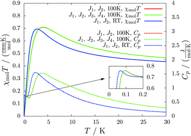
For molecule 1 Merhi et al.²¹ obtained a coupling constant of 1.6 cm⁻¹ by fitting the experimental data to a simple Heisenberg chain model including interchain interactions in an abstract, effective manner. However, the authors observed deviations from a theoretical investigation of that system.¹⁸ These discrepancies are mainly caused by geometrical differences, but are also rooted in the fact that the calculations considered only a single coupling and not a combination of interactions, which is present in the structure.

Our analysis yields a much more detailed picture. The BS calculations for the structure measured at 100 K reveal a larger coupling constant of J₁ = 5.4 cm⁻¹ than obtained by Merhi et al., which is countered by an antiferromagnetic interchain coupling of J₂ = −0.5 cm⁻¹. The latter coupling connects pairs of chains forming a 1D spin ladder. We found that further couplings (J₃ = 0.1 cm⁻¹, J₄ = −0.1 cm⁻¹) basically do not change the resulting magnetic susceptibility and magnetic heat capacity for this system, which is shown by the coinciding red and green lines in Fig. 5.

Fig. 5 The temperature-dependent magnetic susceptibility, plotted as molar susceptibility times temperature (solid curves), and magnetic heat capacity (dashed curves) for different magnetic models of system 1. Results for the structure measured at 100 K are compared to one obtained at room temperature (RT). The inset shows the heat capacity at tiny temperatures.

The results for the crystal structure obtained at room temperature are very similar to those for the low-temperature structure (blue lines in Fig. 5). Due to the larger distance between the molecules all coupling constants are weakened so that J₁ = 3.5 cm⁻¹ and J₂ = −0.3 cm⁻¹. All qualitative features stay the same. Because the couplings influence the data at low temperatures much more than at high temperatures we consider the data obtained for the low-temperature structure to be more reliable. However, working with a crystal structure measured at room temperature is still reasonable, because the ratio of different coupling constants and the overall magnetic structure are not severely affected.

According to our results, the description of the system at low temperatures is not complete if only the ferromagnetic interaction is considered. The small antiferromagnetic coupling leads to a decrease of the susceptibility at very low temperatures. Furthermore, a second maximum in the heat capacity curves indicates an antiferromagnetic phase at temperatures below 0.1 K.

Another literature example,²⁹ where our results agree with the experimental data, is discussed in the ESI.†

4.2 Compound 2: R = anthracenyl

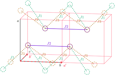
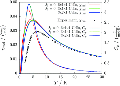
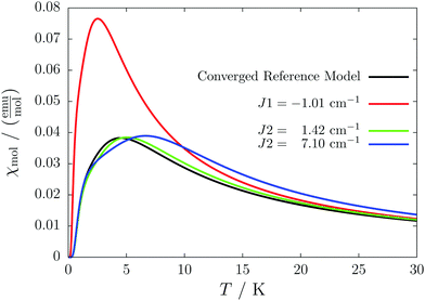
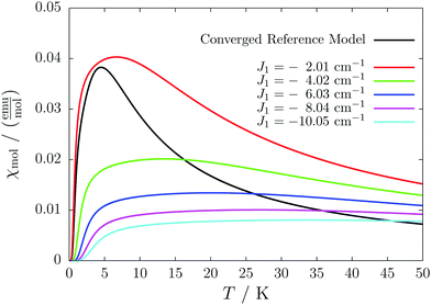
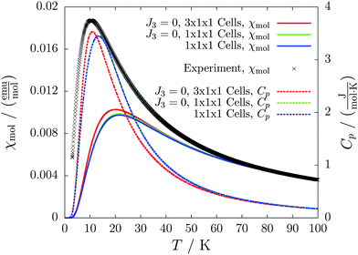
For the radical with an anthracenyl substituent (2 in Fig. 1) we obtained three different coupling constants: J₁ = −2.0 cm⁻¹, J₂ = 0.7 cm⁻¹ and J₃ = −0.1 cm⁻¹. The strongest coupling traverses the system in a zig-zag manner. J₂ is oriented into the same direction and connects the edges of the zig-zag chain formed by J₁ in a straight line. In combination these couplings form a magnetic structure similar to a spin ladder. The weaker antiferromagnetic coupling loosely connects different ladders in a zig-zag fashion promoting the dimensionality of the system from 1D to 2D. This magnetic structure is illustrated in Fig. 6. The ground state of this system is spin compensated. Although in the lowest-energy state each side of the ladder is a line of spins with the same orientation due to J₂, the rungs of the ladder (J₁) lead to opposing spins of the sides. As the convergence checks indicate, J₃ has an insignificant contribution to the magnetism of the system (see the blue and green lines in Fig. 7). If J₃ is respected, convergence has to be tested into two directions. If the model is instead enlarged only into the direction of J₁ and J₂ one can see that the chosen model respecting J₃ is not yet converged into that direction. By extending the model further into that direction (red curves) the error quickly drops below one percent. Still, already the smaller magnetic models show qualitative agreement with the experimentally measured curve. The predicted magnetic heat capacity (dashed lines) reveals a transition from the antiferromagnetic to the paramagnetic phase at about 3 K.

Fig. 6 The magnetic structure of compound 2. Additional to the magnetic unit cell (red) the original cell vectors a, b, and c are shown in black. The directions into which the magnetic model is extended (a′ and b′) coincide with these. Each circle denotes the center of mass of a molecule. Interactions shown by dashed lines are leaving the two depicted cells.

Fig. 7 The temperature-dependent molar magnetic susceptibility (solid lines) compared with the experimental data (black crosses), and the temperature-dependent magnetic heat capacity (dashed lines) for different magnetic models of compound 2.

This detailed analysis of the magnetic structure yields an increased understanding of the underlying processes which can be further exploited. We have seen that J₁ is the dominating coupling in this system as the overall magnetic behavior is antiferromagnetic. This is not only due to its strength, but also due to the way it is built into the magnetic structure. With a simple computer experiment we can confirm this observation. If we want to tune the system more towards ferromagnetism (or away from antiferromagnetism) by manipulating the coupling constants we could either reduce the strength of J₁ or raise the strength of J₂. From what we have learned about the system it is obvious that raising J₂ only has a minor effect. As long as the sides of the ladder have opposing spin it does not matter how strong the coupling within each of the sides is. The results shown in Fig. 8 clearly demonstrate that halving J₁ has a much stronger effect on the system than doubling J₂. Effectively, J₁ defines a temperature below which the system becomes antiferromagnetic irrespective of J₂. This can be emphasized by a rather extreme example. We set J₂ to a very high value of 1000 cm⁻¹. One may expect a coupling strength of about 10 cm⁻¹ to be negligible in the presence of such a strong coupling. In contrast to this expectation, Fig. 9 shows that J₁ still dominates the susceptibility curve up to a temperature which depends only on J₁ and not on J₂.

Fig. 8 Impact of changing the strength of J₁ and J₂ in compound 2. Halving J₁ (red) has a much more pronounced effect on the susceptibility than increasing J₂ by a factor of 2 (green) or 10 (blue). The data obtained with the original values is shown as a reference (black).

Fig. 9 The magnetic susceptibility of a system derived from compound 2 with an artificially large ferromagnetic coupling constant of J₂ = 1000 cm⁻¹ for different values of J₁. The data obtained with the original values is shown as a reference (black).

4.3 Compound 3: R = 4-(diphenylamino)phenyl

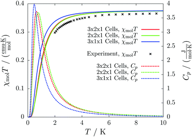
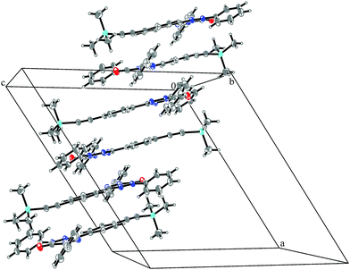
System 3 consists of four non-negligible couplings: J₁ = −0.7 cm⁻¹, J₂ = 0.4 cm⁻¹, J₃ = 0.1 cm⁻¹ and J₄ = 0.1 cm⁻¹. J₁ and J₂ form an alternating chain in a zig-zag manner along the bc diagonal of the unit cell. J₃ and J₄ loosely connect these chains to form a net. We refrain from illustrating the magnetic topology here, because the magnetic unit cell appears too busy to create a helpful representation.

These couplings are significantly smaller than the couplings observed in the other systems studied in this work. Considering the crystal structure (see Fig. 10) it is clear that the bulky diphenylamino substituent prevents an efficient stacking of the π-systems. As a consequence, the strongest coupling is between the twisted N-phenyl groups of the verdazyl rings and the oxygen atoms, which have a distance of almost 4 Å to each other. The stacking interaction of the π-systems (J₂) is very weak, not primarily due to the distance of 3.41 Å between the closest atoms, but mainly because the corresponding phenyl rings are displaced.

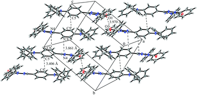Fig. 10 Packing diagram of verdazyl radical 3. Displacement ellipsoids are shown with 30% probability.

The results for different magnetic models quickly converge to errors far below one percent and agree with the experimental curve as depicted in Fig. 11. The heat capacity indicates a transition at a temperature below 1 K. Thus experimentally only paramagnetism can be observed.

Fig. 11 The temperature-dependent magnetic susceptibility, plotted as molar susceptibility times temperature (solid lines) compared with the experimental curve (black crosses), and the temperature-dependent magnetic heat capacity (dashed lines) for different magnetic models of compound 3.

4.4 Compound 4: R = p-trimethylsilylethynylphenyl

This compound is a derivate of 1, where the original methyl substituents at the verdazyl ring have been replaced by phenyl groups and a TMS protecting group is attached to the ethynylphenyl substituent of the verdazyl ring.

The magnetic structure is an approximately linear chain with alternating antiferromagnetic (J₁ = −11.9 cm⁻¹) and ferromagnetic (J₂ = 11.2 cm⁻¹) couplings, which is oriented along the ac direction of the unit cell as depicted in Fig. 12. J₁ is caused by the formation of an antiparallelly oriented dimer (see Fig. S3 and S4 in the ESI†). Similar to compound 1 the π-systems have a distance of about 3.4 Å to each other. J₂ is the stacking interaction connecting different dimers (see Fig. S5 in the ESI†), which are severely twisted against each other by an angle of about 160°. Here, the closest contacts are between the nitrogen atoms of the verdazyl rings with a distance of 3.29 Å.

Fig. 12 Packing diagram of verdazyl radical 4. The antiparallel dimers (J₁) stack upon each other, enabling the interaction J₂, to form a chain along the ac diagonal of the crystal. Displacement ellipsoids are shown with 30% probability.

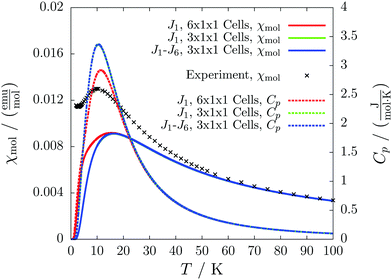
The chains are further loosely connected by a weak antiferromagnetic coupling (J₃ = −0.6 cm⁻¹). In the pictorial representation (Fig. 13) we neglect the latter for convenience. The very similar susceptibilities for a small model (green and blue solid lines in Fig. 14) and the coinciding heat capacity curves (green and blue dashed lines in Fig. 14) indicate that J₃ is by far less relevant than the other couplings.

Fig. 13 The magnetic structure of compound 4, neglecting the small interchain coupling J₃. Only one of the two identical chains is shown. For comparison, the unit cell with its original cell vectors is shown in black. Each circle denotes the center of mass of a molecule. Interactions shown by dashed lines are leaving the two depicted magnetic cells.

Fig. 14 The temperature-dependent molar magnetic susceptibility (solid lines) compared with the experimental curve (black crosses), and the temperature-dependent magnetic heat capacity (dashed lines) for different magnetic models of compound 4.

For this system the convergence checks are problematic, because the unit cell already contains eight molecules. Thus, with our chosen settings only a single unit cell could be modeled. Fortunately, when neglecting J₃ the cell comprises two separate chains. Our program automatically treats the—in this case identical—chains completely separately. In this way, we can observe sufficient convergence by enlarging the model along the chain towards three magnetic unit cells (red lines in Fig. 14).

We clearly observe an antiferromagnetic system with a transition to the paramagnetic phase at about 11 K.

4.5 Compound 5: R = p-ethynylphenyl

Despite the similarity in the structure of this molecule with the verdazyl radical 1, the different packing in the crystal structure inverts the character of that compound. The magnetic structure is an antiferromagnetically coupled Heisenberg chain (J₁ = −8.4 cm⁻¹) with five smaller interactions with a strength of up to 0.3 cm⁻¹. Among the smaller couplings is also the head-to-tail interaction (see the packing diagram in Fig. S7 in the ESI†). As can be seen by the coinciding green and blue curves in Fig. 15 none of these additional couplings are relevant for the macroscopic behavior. The converged model (red curves) indicates a transition from the antiferromagnetic to the paramagnetic phase at about 11 K. The deviation to the experimental curve at very low temperatures might be due to paramagnetic impurities.

Fig. 15 The temperature-dependent molar magnetic susceptibility (solid lines) compared with the experimental curve (black crosses), and the temperature-dependent magnetic heat capacity (dashed lines) for different magnetic models of compound 5.

The stacking interaction J₁ is illustrated in Fig. 16 (for a top view see Fig. S8 in the ESI†). The orientation of the molecules and the corresponding distances allow for a π–π interaction. The closest contact with a distance of 3.30 Å is between the oxygen atom of one verdazyl radical and the carbon atom which is substituted with the ethynylphenyl moiety. This distance is slightly smaller than for radical 1 (3.40 Å) and rationalizes the larger coupling strength. At the same time the larger distance between the verdazyl ring centroids (5.34 Å compared to 4.06 Å) and the corresponding larger slip is most probably responsible for the inversion of the character of J₁.

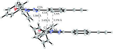Fig. 16 The pair of molecules in the crystal structure of verdazyl radical 5 which is responsible for the stacking interaction J₁. Displacement ellipsoids are shown with 30% probability.

5 Discussion and conclusions

In this work, we presented a robust and easy-to-use procedure to calculate magnetic susceptibility vs. temperature curves and corresponding magnetic heat capacities based on crystal structures of organic radicals. It can be applied to all spin-1/2 systems in which each spin site is a clearly separated molecule or complex within the crystal structure. The procedure can be straightforwardly extended to systems with higher spin.

We applied the strategy to a number of novel verdazyl radicals. The presented results show that qualitative results can reliably be achieved by our method. Magnetic model sizes which can still be treated in a short amount of time on a desktop computer are typically sufficient to obtain converged results. Still, full quantitative agreement with the experiment is often not achieved. In some cases (e.g. for system 2) an unconverged model agrees better with the experimental results than the converged one. In such cases it is tempting to use the unconverged model. The reason for the better agreement clearly is an unsystematic error cancellation so that non-converged models should not be used for interpretation if better converged models are available.

We have seen that the results are often more sensitive to the magnetic topology than to particular coupling constants. Because all qualitative features can be reproduced also with inaccurate coupling constants, the generated models and the quantum mechanically calculated coupling constants are an ideal starting point for a fitting procedure with which the coupling constants may be further refined. To obtain more accurate coupling constants directly from the quantum chemical calculations, or in cases the BS-DFT approach fails (as e.g. shown in ref. 13), expensive multideterminantial wave function methods have to be employed. Improved results can, for example, be obtained from complete active space self consistent field (CASSCF) calculations with additional treatment of dynamical correlation effects by means of perturbation theory⁴² or truncated configuration interaction (CI) methods like the difference-dedicated CI by Malrieu and co-workers⁴³ or the modified CAS-CI by Fink and Staemmler.⁴⁴ As an alternative to computationally expensive wavefunction methods, empirical scaling factors can be applied on top of BS-DFT calculations,⁴⁵ although additional to a functional dependence also a possible system dependence needs to be considered. Further factors affecting the coupling constants could be the presence of other molecules during the calculation of the interaction between a pair of molecules and also temperature effects, as observed by Merhi et al.²¹ and confirmed in this work.

If a system cannot be described with sufficient accuracy by the Heisenberg Hamiltonian shown in eqn (2), the approach used by us is bound to fail. Advanced Hamiltonians, which include three-body terms or take anisotropies into account,⁴ or a spin transition model⁴⁶ need to be applied in such cases. However, despite this limitation and the inaccuracies in the coupling constants, our approach provides excellent explanations of the microscopic processes leading to the macroscopically observed properties for all systems we investigated so far.

In summary, the results obtained by applying our presented black-box method for magnetic susceptibilities agree qualitatively with experimental data. A lot of insight can be gained into the magnetic structure, which causes the macroscopic magnetic behavior. Whether the results are sensitive to specific coupling constants is determined by the way the coupling is built into the magnetic structure. In that way the effect of a strong coupling can be significantly diminished by a much smaller coupling with opposing sign.

Conflict of interest

The authors declare that they have no conflict of interest.

Acknowledgements

This work was supported by the Deutsche Forschungsgemeinschaft (DFG) through the Collaborative Research Center SFB 858. We thank Prof. K. Awaga and Assoc. Prof. M. M. Matsushita for an IRTG Münster-Nagoya research internship in the Research Center for Materials Science at the Nagoya University (Japan); furthermore we are thankful for the opportunity to perform some magnetic susceptibility measurements and for helpful discussions.

References

1. M. Kaupp, M. Bühl, and V. Malkin, Calculation of NMR and EPR Parameters: Theory and Applications, Wiley, 2004.
2. J. J. Novoa, M. Deumal and J. Jornet-Somoza, Chem. Soc. Rev., 2011, 40, 3182.
3. M. Deumal, M. J. Bearpark, J. J. Novoa and M. A. Robb, J. Phys. Chem. A, 2002, 106, 1299.
4. A. V. Postnikov, J. Kortus and M. R. Pederson, Phys. Status Solidi B, 2006, 243, 2533.
5. J. P. Malrieu, R. Caballol, C. J. Calzado, C. de Graaf and N. Guihéry, Chem. Rev., 2014, 114, 429.
6. H. Lueken, Magnetochemie: Eine Einführung in Theorie und Anwendung, Teubner Studienbücher Chemie, Vieweg + Teubner Verlag, Stuttgart – Leipzig, 1999, p. 135f.
7. Y. Shao, M. Head-Gordon and A. I. Krylov, J. Chem. Phys., 2003, 118, 4807.
8. Z. Rinkevicius and H. Ågren, Chem. Phys. Lett., 2010, 491, 132.
9. H. Zhekova, M. Seth and T. Ziegler, J. Chem. Theory Comput., 2011, 7, 1858.
10. N. J. Mayhall and M. Head-Gordon, J. Chem. Phys., 2014, 141, 134111.
11. N. J. Mayhall and M. Head-Gordon, J. Phys. Chem. Lett., 2015, 6, 1982.
12. L. Noodleman, J. Chem. Phys., 1981, 74, 5737.
13. M. Fumanal and M. Deumal, Phys. Chem. Chem. Phys., 2016, 18, 20738.
14. J. Kortus, C. S. Hellberg and M. R. Pederson, Phys. Rev. Lett., 2001, 86, 3400.
15. D. A. Pantazis, M. Orio, T. Petrenko, S. Zein, E. Bill, W. Lubitz, J. Messinger and F. Neese, Chem. – Eur. J., 2009, 15, 5108.
16. C. Baffert, M. Orio, D. A. Pantazis, C. Duboc, A. G. Blackman, G. Blondin, F. Neese, A. Deronzier and M.-N. Collomb, Inorg. Chem., 2009, 48, 10281.
17. S. Vela, M. Deumal, M. M. Turnbull, and J. J. Novoa, A theoretical analysis of the magnetic properties of the low-dimensional copper(II)X2(2-X-3-methylpyridine)2 (X = Cl and Br) complexes, in 8th Congress on Electronic Structure: Principles and Applications (ESPA 2012), ed. J. J. Novoa and M. F. Ruiz López, Highlights in Theoretical Chemistry, Springer, Berlin Heidelberg, 2014, vol. 5, pp. 219–230.
18. J.-B. Rota, B. L. Guennic and V. Robert, Inorg. Chem., 2010, 49, 1230.
19. K. C. Ko, D. Cho and J. Y. Lee, J. Phys. Chem. A, 2012, 116, 6837.
20. C. P. Constantinides, P. A. Koutentis and J. M. Rawson, Chem. – Eur. J., 2012, 18, 7109.
21. A. Merhi, T. Roisnel, S. Rigaut, C. Train and L. Norel, CrystEngComm, 2014, 16, 9783.
22. I. Ratera and J. Veciana, Chem. Soc. Rev., 2012, 41, 303.
23. B. D. Koivisto and R. G. Hicks, Coord. Chem. Rev., 2005, 249, 2612.
24. S. J. Blundell and F. L. Pratt, J. Phys.: Condens. Matter, 2004, 16, R771.
25. J. S. Miller and A. J. Epstein, MRS Bull., 2000, 25, 21.
26. M. Kinoshita, Jpn. J. Appl. Phys., 1994, 33, 5718.
27. S. Eusterwiemann, D. Matuschek, L. Stegemann, S. Klabunde, C. Doerenkamp, C. G. Daniliuc, N. L. Doltsinis, C. A. Strassert, H. Eckert and A. Studer, Chimia, 2016, 70, 172.
28. D. Matuschek, S. Eusterwiemann, L. Stegemann, C. Doerenkamp, B. Wibbeling, C. G. Daniliuc, N. L. Doltsinis, C. A. Strassert, H. Eckert and A. Studer, Chem. Sci., 2015, 6, 4712.
29. M. Vérot, N. Bréfuel, J. Pécaut, C. Train and V. Robert, Chem. – Asian J., 2012, 7, 380.
30. C. Herring, Direct exchange between well-separated atoms, in Magnetism, Part IIB, ed. G. T. Rado and H. Suhl, Academic Press, New York – London, 1966, p. 5.
31. M. Mantina, A. C. Chamberlin, R. Valero, C. J. Cramer and D. G. Truhlar, J. Phys. Chem. A, 2009, 113, 5806.
32. F. Neese, Wiley Interdiscip. Rev.: Comput. Mol. Sci., 2012, 2, 73.
33. C. Adamo and V. Barone, J. Chem. Phys., 1999, 110, 6158.
34. J. Zheng, X. Xu and D. Truhlar, Theor. Chem. Acc., 2011, 128, 295.
35. K. Eichkorn, O. Treutler, H. Öhm, M. Häser and R. Ahlrichs, Chem. Phys. Lett., 1995, 240, 283.
36. E. R. Davidson, J. Comput. Phys., 1975, 17, 87.
37. C. Lanczos, J. Res. Natl. Bur. Stand., 1950, 45, 255.
38. K. Park, M. R. Pederson and C. S. Hellberg, Phys. Rev. B: Condens. Matter Mater. Phys., 2004, 69, 014416.
39. E. Ruiz, T. Cauchy, J. Cano, R. Costa, J. Tercero and S. Alvarez, J. Am. Chem. Soc., 2008, 130, 7420.
40. Y. Masuda, M. Kuratsu, S. Suzuki, M. Kozaki, D. Shiomi, K. Sato, T. Takui and K. Okada, Polyhedron, 2009, 28, 1950.
41. G. A. Bain and J. F. Berry, J. Chem. Educ., 2008, 85, 532.
42. C. Angeli, R. Cimiraglia, S. Evangelisti, T. Leininger and J.-P. Malrieu, J. Chem. Phys., 2001, 114, 10252.
43. J. Miralles, O. Castell, R. Caballol and J.-P. Malrieu, Chem. Phys., 1993, 172, 33.
44. K. Fink and V. Staemmler, Mol. Phys., 2013, 111, 2594.
45. D. Cho, K. C. Ko and J. Y. Lee, Int. J. Quantum Chem., 2016, 116, 578.
46. L. Norel, J.-B. Rota, L.-M. Chamoreau, G. Pilet, V. Robert and C. Train, Angew. Chem., Int. Ed., 2011, 50, 7128.

---

Footnote

† Electronic supplementary information (ESI) available. CCDC 1497165 (3), 1497166 (4) and 1497167 (5). For ESI and crystallographic data in CIF or other electronic format see DOI: 10.1039/c6cp05875b

---