Entanglements in polymer nanocomposites containing spherical nanoparticles

Abstract

We investigate the polymer packing around nanoparticles and polymer/nanoparticle topological constraints (entanglements) in nanocomposites containing spherical nanoparticles in comparison to pure polymer melts using molecular dynamics (MD) simulations. The polymer–nanoparticle attraction leads to good dispersion of nanoparticles. We observe an increase in the number of topological constraints (decrease of total entanglement length N_e with nanoparticle loading in the polymer matrix) in nanocomposites due to nanoparticles, as evidenced by larger contour lengths of the primitive paths. An increase of the nanoparticle radius reduces the polymer–particle entanglements. These studies demonstrate that the interaction between polymers and nanoparticles does not affect the total entanglement length because in nanocomposites with small nanoparticles, the polymer–nanoparticles topological constraints dominate.

---

1 Introduction

The dynamics of long polymers is controlled by entanglements, which are topological constraints imposed by the other chains. These can dramatically change the polymer viscosity, dynamics, mechanical and tribological properties. In this paper we explore how spherical nanoparticles affect rheology by studying the entanglements in polymer–nanoparticle composites in the cases when the polymer radius of gyration (R_g) is larger than^1–4 or of the order of the nanoparticle diameter (D).^5–9

The quality of nanoparticle dispersion^10,11 can play an important role on the polymer structure thus on polymer entanglements. In a well dispersed polystyrene (PS) chains/(PS) nanoparticles nanocomposite,¹² neutron scattering showed polymer chain expansion for polymer chains with radius of gyration larger than the nanoparticle radius (R), similar to the study of poly(dimethylsiloxane)/polysilicate nanocomposites.¹³ This has also been observed recently by simulations^14,15 and a thermodynamic model¹⁶ but it is contrary to other recent studies of PS/silica^10,11,17 nanocomposites where polymers are unperturbed, and in poly(ethylene-propylene)(PEP)/silica nanocomposites⁵ where the polymer chains are contracted at very high nanoparticle loading; however, in some of the previous studies^10,17 good nanoparticle dispersion has not been achieved and in some others^5,13 transmission electron microscopy (TEM) data were not reported, so the extent of dispersion is unknown.

Spherical nanoparticles can affect the primitive path and entanglement network of long polymers.¹⁸ An increase of the entanglement polymer density is the origin of mechanical reinforcement in nanocomposites.^19–23 In particular it was shown using a slip-link model,²⁴ that in nanocomposites with “bare” fillers, a relatively small level of reinforcement was evidenced,²³ which is not verified in PS/silica and poly(methyl-methacrylate)/silica nanocomposites.²⁵ In addition, in ref. 23 was shown that the viscosity of the nanocomposite, η, seems to be independent of the state of dispersion and can be predicted by the classical Einstein law: η = η₀(1 + 2.5)ϕ (where η₀ is the viscosity of the pure polymer melt, and ϕ is the nanoparticle volume fraction). However, the reinforcement is considerably higher when nanocomposites contain nanoparticles with grafted chains.²³ Such an observation was also reported recently by molecular dynamics simulations.²⁶ In addition, other parameters may also play a role on mechanical reinforcement such as size and shape of fillers, polymer matrix, interaction between fillers and matrix, and computer simulations^{20,21,27–31} have been used extensively to answer that fundamental problem.

The geometry of the nanoparticle (such as buckyball, graphene, nanodiamond^32,33 or nanorod^34–36) can also affect the polymer/nanoparticle entanglement network. However in most of the entanglement network studies, a dilute nanoparticle regime^{32–34,36–38} has been investigated, in which the polymer entanglement network, excluding the nanoparticles, remains unaffected. Only the MD study of nanoparticles R = 5 (where R_g ≈ D)³⁹ and Monte Carlo (MC) study by Termonia,^40,41 have been performed at nanoparticle loadings above percolation. It is worthy to note that the MC study^40,41 is based on a body-centered-cubic (bcc) lattice in which the nanoparticles are fixed, and the polymer free volume remains constant irrespective of the nanoparticle size, which is not the real case in an experiment.^5,42,43

In this article, we investigate the polymer packing (free volume) in nanocomposites which contain spherical nanoparticles as fillers. We calculate the number of monomers between entanglements, entanglements per chain⁴⁴ and primitive path (the shortest path connecting the two ends of the polymer chain subject to the topological constraints)⁴⁵ in both polymer melts and nanocomposites of oligomers and weakly entangled polymers by using topological algorithms^44,46–48 and applying different entanglements estimators.⁴⁷ The rest of this paper is organized as follows. In Section 2, the theoretical background is given for the entanglement analysis that is implemented in polymer melts and polymer nanocomposites. In Section 3, we discuss first the primitive path and entanglements of the polymer model used in this study. In polymer nanocomposites, we investigate the free volume and entanglements as a function of polymer molecular weight, volume fraction of fillers, interaction of polymers with fillers and nanoparticle radius in comparison to theoretical relations. Finally, in Section 4, conclusions are presented.

2 Estimators for entanglement length N_e

In polymer melts of sufficiently long flexible chain molecules, neighboring chains strongly interpenetrate and entangle with each other.⁴⁹ Thus, the motion of polymers whose degree of polymerization is greater than the “entanglement length” N_e is confined to a tube-like region.

The N_e is determined by the estimator of Everaers et al.⁴⁵ (which we denote as classical S-coil), evaluated using the geometrical Z1 algorithm.^44,46–48 This N_e estimator is determined by statistical properties of the primitive path as a whole coil and evaluated for a given number of monomers N in the polymer chain as follows:

where R_ee is the end-to-end vector distance of a polymer chain and L_pp is the contour length of its primitive path, the averages are taken over the ensemble of chains.

Another estimator for the entanglement length can be used by measuring the number of interior “kinks”^44,46 which is considered to be proportional to the number of entanglements. The estimator on the number of “kinks”, 〈Z〉, is denoted here as classical S-kink is given by:⁴⁴

In addition, there are modified estimators that provide an upper bound for N_e, such as the modified S-coil,⁴⁷ but they tend to overestimate N_e for weakly entangled chains:

In order to eliminate the systematic errors that appear in the previous estimators⁴⁷ and to obtain an accurate N-independent value, we use an ideal N_e estimator (M-coil),⁴⁷ which requires simulation of multiple systems of different chain lengths, using coil properties:

where C(x) ≡ 〈R_ee²〉/R_RW²(x) is the characteristic ratio⁵⁰ for a chain with x monomers, and R_RW²(x) = (x − 1)r₀² is the reference mean squared end-to-end distance of a random walk, where r₀ = 0.967. Because of the dependence of C(x) on the number of monomers x, this estimator can be applicable to non-Gaussian chains. This non-Gaussian statistics of chains and primitive paths produces systematic errors in the old estimators for N_e such as eqn (1).⁵¹ The M-coil estimator converges faster than eqn (1) and (3) because it uses information from a series of polymer chains, while the S-coil one uses only information from a single polymer chain length. More discussion and details regarding the N_e estimators can be found in ref. 47. The averages in our analysis are taken over the ensemble of all chains at each time step. Then the time average is taken for 400–2000 saved configurations depending of the length size (at a time larger than the disentanglement time: τ_d, τ_d = (N/N_e)³τ_Rouse(N_e) ≈ 185 000τ for N = 200, where τ_Rouse(N_e) = 5000τ is obtained for semiflexible polymers from Fig. 9 in ref. 52).

3 Results and discussion

3.1 Polymer melt

The chain and primitive path dimensions as calculated from the Z1 algorithm^44,46–48 for the polymer melts, of the semiflexible model used in this study, are presented in Table 1.

Table 1 Number of polymers in the simulation cell (N_p), monomers in a polymer chain (N), length of the simulation cell (L) measured in units of the monomer diameter σ_m, square end-to-end vector distance 〈R_ee²〉, contour length of the primitive path L_pp, and number of “kinks” 〈Z〉. Radius of gyration of polymers with N = 200: R_g ≈ 8

N p	N	L	R ee ^2	L pp	〈Z〉
6000	10	41.328	15.2	3.75	0.02
3000	20	41.328	34.24	5.93	0.25
1250	40	38.891	69.29	9.82	0.94
1200	50	41.328	93.25	11.65	1.27
600	80	38.365	152.9	17.7	2.23
6000	100	41.328	190.98	20.58	2.78
300	160	38.365	313.4	32.05	3.51
118	200	30.454	389	37.59	5.4 ± 0.3

---

We depict the behavior of the M-coil estimator (eqn (4)) for the semiflexible Kremer–Grest (KG) polymer model studied, in Fig. 1, in comparison with results⁴⁷ of the fully flexible KG model.⁵³ From Fig. 1, it can be extracted that for the polymer model used in this study, N_e ≈ 59.7, while the value obtained from the S-coil estimator (eqn (1)) is 54.9. Other methodologies than the primitive path analysis, such as mean square displacement measurements (MSD),^51,54 can predict a much different N_e value.^51,54 The MSD methodology assumes validity of the reptation model and assumptions made to come up with the numerical prefactors. By adding an intrinsic bending potential⁵² the Kuhn length,⁴⁹l_k, increases (for the polymer model used: l_k = 〈R_ee²〉/L_c = 2.02, where L_c is the contour length of the polymer chain) and the packing length p⁴⁵ (the characteristic length at which polymers start to interpenetrate) decreases, thus the N_e value unavoidly decreases for a semiflexible model⁵⁵ in comparison to the fully flexible Kremer–Grest model.⁵³ The glass transition of a polymer model which contains a bending potential (but not a torsional potential) is T_g = 0.4.⁵²

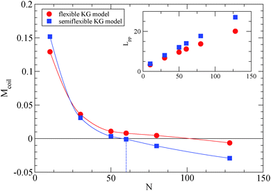Fig. 1 Simulations yield N_e for the semiflexible polymer model used in this study estimated from the M-coil estimator (eqn (4)). Solid lines interpolating between data points have been added to guide the eye. For comparison, MD simulations of fully flexible Kremer–Grest model (circles)⁵³ are included. Inset: Dependence of L_pp for different polymers in the frozen particle limit.

3.2 Nanocomposites

For nanocomposites, we consider systems of spherical nanoparticles in a dense polymer melt. In the nanocomposite systems studied, a total number of N_t = 23 600 monomers were used in a cubic cell with nanoparticles of radius R = 1 or 2 (in nanocomposites with nanoparticles R = 4 and polymer matrices N ≤ 160, N_t = 9440 monomers were used, whereas for R = 4 and polymer matrices N = 200 the total number of monomers was N_t = 23 600). We define the nanoparticle (filler) volume fraction ϕ in our simulations as , where D is the nanoparticle diameter and 〈V〉 is the total average volume of the nanocomposite simulation box during the NPT simulation. The mass of nanoparticle is m = 0.85πD³/6. Details of the nanocomposite systems studied (equilibration, length of the simulations) are given in ref. 14 and in Table 2.

Table 2 Nanoparticle volume fraction ϕ (%), simulation cell average length 〈L〉 measured in units of the monomer diameter σ_m, number of nanoparticles N_n, radius of nanoparticles R, measured in units of the monomer diameter, for nanocomposites. The ϕ (%), 〈L〉, correspond to nanocomposites with attractive nanoparticles R = 1 (ϕ (%) and 〈L〉 of the other nanocomposites can be found in ESI). In nanocomposites with R = 4 and polymer matrix: N = 200 at ϕ ≈ 10.7, 19.5, 26.9%, the number of nanoparticles embedded in the polymer matrix were N_n = 12, 25, 37 respectively

ϕ (%)	L(σm)	N n
		R = 1	R = 2	R = 4
5.5	31.157	400	—	—
10.3	31.863	800	100	5
14.5	32.569	1200	—	—
18.2	33.282	1600	200	10
24.2	34.653	2400	300	15
36	38.53	4906	—	—

---

In the next sections we investigate the effect of nanoparticle volume fraction, polymer–nanoparticle interaction and nanoparticle radius on the entanglement length N_e and primitive path. In the nanocomposite systems studied we consider the case of the primitive path analysis for both the frozen particle limit, where nanoparticles are held fixed in space during the primitive path analysis, and the phantom particle limit. In the phantom particle limit nanoparticles are unable to restrict polymer motion on the time scales relevant to reptation dynamics. We approximate this limit, by removing the nanoparticles from the simulated system prior to the primitive path analysis. In the frozen particle limit, the N_e contains two types of entanglements: polymer–polymer and polymer–nanoparticle entanglements, whereas in the phantom limit, it contains only polymer–polymer entanglements.

3.2.1 Effect of nanoparticle loading on polymer density. Nanocomposites with nanoparticles of R = 1 are similar to experimental systems of POSS nanoparticles (R = 1 nm) dispersed in polymer matrix (such as poly(ethylene-alt-propylene)).⁵⁶ Since we perform NPT simulations where the volume of the simulation box 〈V〉 fluctuates, the monomer density fluctuates and we can consider free volume effects. The quantification of free volume can be measured by calculating the net packing fraction (NPF):where 〈V〉 is the simulation average volume, N_n the number of nanoparticles, N_t is the total number of monomers, and σ_m is the monomer diameter.

As can be seen in Fig. 2, the net packing fraction can increase (free volume decreases) as nanoparticle loading increases. This effect becomes stronger by dispersing large nanoparticles as also reported in ref. 57. While in ref. 57 only the dilute nanoparticle loading has been explored, we show the net packing fraction for a wider nanoparticle concentration range. The polymer nanoparticle interaction alters the free volume dramatically in the case of small nanoparticles R = 1. Since the smaller nanoparticles have a high interfacial area which increases with the nanoparticle loading, it is shown that the interfacial area is a factor that controls the packing fraction of such nanocomposite. However in nanocomposites containing larger attractive nanoparticles such as of size R = 4, the interfacial area diminishes and does not contribute to the net packing fraction. The polymer matrix has a slight effect on NPF calculations (shown in Fig. 2), an unentangled polymer matrix can reduce slightly the net packing fraction of the nanocomposites for all nanoparticle loadings. By dispersing attractive nanoparticles in the polymer matrix the polymer density around the nanoparticles increases.¹⁴ By tuning the polymer–nanoparticle interaction ε_mp, not only the interface but also the dispersion and aggregation behavior (which have been explored by molecular dynamics simulations^14,21,58,59) of the nanoparticles in nanocomposites is altered. It was shown that attractive nanoparticles of radii R = 1–4 can be dispersed in an unentangled or entangled polymer matrix (R_g/R ≈ 0.4–8)¹⁴ in agreement to previous simulation studies.²¹ However, for repulsive polymer nanoparticle interaction, poor dispersion is observed for R_g/R ≈ 0.4–4 (in our case radii R = 2 to R = 4),¹⁴ which has also been observed experimentally for systems with weak interactions such as polystyrene–silica nanocomposite^10,17 and possibly for a repulsive nanoparticle nanocomposite such as PEP–silica.⁵

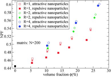Fig. 2 Net packing fraction for polymers of N = 200, calculated using eqn (5), for different nanoparticle loading and radius for repulsive (filled symbols) and attractive (open symbols) nanoparticles. (i) Polymer melt (black square), (ii) R = 1 (red squares), (iii) R = 2 (green diamonds), (iv) R = 4 (blue circles). The star symbols denote the NPF for nanocomposites containing R = 1 attractive nanoparticles in unentangled (N = 10) polymer matrix.

3.2.2 Effect of nanoparticle loading on entanglement length N_e. The modified S-coil, classical S-coil, and S-kink estimators (eqn (1)–(3)) for determining N_e are applied on the nanocomposite systems, and shown in Fig. 3 for two nanoparticle loadings and nanoparticle size of R = 1. In general, both S-coil, S-kink (eqn (1) and (2) respectively) and modified S-coil estimators (eqn (3)) cannot correctly predict the N_e value for all N exceeding N_e. Eqn (1) and (2) converge to N_e value slowly with increasing N, whereas eqn (3) tends to approach N_e from above rather than from below, but overestimating its value for weakly entangled chains. However, they clearly show the effect of the volume fraction on the behaviour of the N_e. In particular, at a nanoparticle loading of 5.5% (inset of Fig. 3), all the estimators show no changes in the N_e value, between the phantom and frozen particle limits, for N = 200. In this case, the nanoparticles do not affect the primitive path of the polymer chains. By increasing the nanoparticle loading above than 5.5%, to 14.5%, it can be seen that the values of all three estimators reduce in the frozen particle limit, in comparison to phantom particle limit. This shows that at such loading, nanoparticles are additional topological constraints, that increase the length of the primitive path and unavoidably decrease the entanglement length. Moreover, (in particular in Fig. 3 from 5.5% to 14.5% loading), it can be seen that the N_e in the phantom limit (red symbols) increases for all polymers. This indicates that small attractive nanoparticles can alter the polymer primitive network. A similar trend, but to a smaller extent, has been also observed at a nanoparticle loading of 10.3% (results not shown). By increasing the nanoparticle loading, there is a higher deviation between the phantom and frozen particle limits, and there is a further decrease of the total entanglement length. In addition to previous estimators, the M-coil estimator (eqn (4)) is used for nanocomposites with small nanoparticles (R = 1) in order to have an N-independent estimation of N_e. Clearly as can be seen in Fig. 4, by increasing the volume fraction of nanoparticles dispersed in the polymer matrix, the N_e is reduced due to the contour length of primitive path, L_pp, increase. It is noted that these N_e values contain two types of entanglements: polymer–polymer and polymer–nanoparticle entanglements. Results from molecular dynamics³⁶ and dissipative dynamics³⁴ simulations of nanorods embedded in a polymer matrix indicate that the inclusion of nanorods into the polymer matrix does not significantly alter the polymer–polymer entanglements network at low nanoparticle loading, instead it creates additional topological constraints of polymer–nanorod origin.

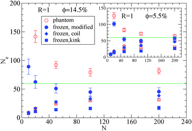Fig. 3 Dependence of N_e using eqn (1), (2) and (3), in the frozen (filled symbols) and phantom (open symbols) particle limits of nanocomposites with attractive small nanoparticles of R = 1, for nanoparticle loading ϕ = 14.5%: (i) modified S-coil estimator: eqn (3) (circles), (ii) classical S-coil estimator: eqn (1) (diamonds), (iii) classical S-kink estimator: eqn (2) (squares). Inset: Estimators for nanoparticle loading ϕ = 5.5%. The green line denotes the N_e for pure polymer melts as extracted by eqn (4).

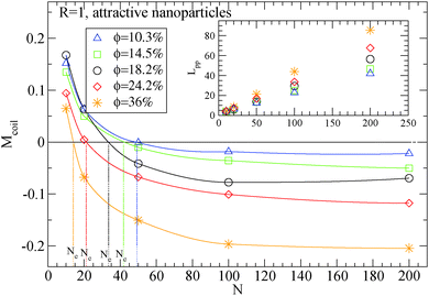Fig. 4 Dependence of N_e using eqn (4) in the frozen particle limit in nanocomposites with attractive small nanoparticles of R = 1 for different nanoparticle loading: (i) 10.3% (triangles), (ii) 14.5% (squares), (iii) 18.2% (circles), (iv) 24.2% (diamonds), (ii) 36% (star symbols). Inset: Dependence of L_pp for different polymers in the frozen particle limit. The vertical lines show the N_e extracted values at each nanoparticle loading.

Moreover, we depict in Table 3, the N_e values (and number of “kinks” 〈Z〉) in the frozen particle limit as calculated by the S-coil, S-kink and S-modified estimators for long polymers N = 200, in nanocomposites at different nanoparticle loading, for both repulsive (Re) and attractive (A) nanoparticles. It can be seen that outside the error margin there is no difference in these N_e (and 〈Z〉) values. The N_e values estimated from M-coil agree with those estimated from S-coil for long polymers (N = 200), within the error margin. Similarly, for nanocomposites consisted of a matrix of polymers N = 100, the type of nanoparticles do not alter the N_e in the frozen particle limit (results not shown). Thus in the case where small nanoparticles are dispersed in a polymer matrix, the polymer–nanoparticle interaction does not play any role on the primitive path. The topological constraints created by nanoparticles seem to dominate the entanglement network even if the polymer dimensions can be altered¹⁴ by the polymer nanoparticle interaction. We also report in Table 3 the number of kinks 〈Z〉 in the phantom limit. We can see that in the phantom limit, 〈Z〉 decreases with nanoparticle loading (whereas it increases in the frozen limit due to polymer nanoparticle entanglements). This shows that nanoparticle loading reduces the polymer–polymer entanglements for nanocomposites containing nanoparticles of radius R = 1.

Table 3 Nanoparticle volume fraction ϕ (%), nanoparticles of radius R = 1 and type: repulsive (Re), attractive (A), polymer matrix: N = 200, N_e(S-coil, S-kink, modified S-coil), number of “kinks” 〈Z〉 in the frozen limit, number of “kinks” in the phantom limit, 〈Z〉(phantom)

ϕ (%)	Type	N e(S-coil)	N e(S-kink)	N e(m.S-coil)	〈Z〉	〈Z〉(ph.)
22.9	Re	18.2 ± 2.1	8.1 ± 0.8	19.4 ± 2.4	23.8 ± 1.9	3.7 ± 0.1
24.2	A	23.2 ± 1.9	7.6 ± 0.7	25.6 ± 2.5	25.6 ± 1.7	4.3 ± 0.1
17.3	Re	32.8 ± 6.5	15.3 ± 3.9	37.2 ± 8.5	12.9 ± 3.5	4.7 ± 0.2
18.2	A	31.8 ± 5.4	11.1 ± 2.5	36.5 ± 7.3	17.7 ± 3.5	4.7 ± 0.2
13.8	Re	44.8 ± 4.9	21.2 ± 3.4	54.6 ± 7.4	8.7 ± 1.8	4.5 ± 0.2
14.5	A	38.6 ± 4.9	17.1 ± 3.1	45.6 ± 7	11.1 ± 2.3	4.8 ± 0.2
10	Re	47.2 ± 2.2	24.9 ± 1.8	57.8 ± 3.4	7.1 ± 0.7	4.9 ± 0.2
10.3	A	47.4 ± 2.3	22.7 ± 1.7	58.3 ± 3.5	7.9 ± 0.7	5.1 ± 0.1
5.4	Re	53.9 ± 3.5	28.8 ± 1.1	68.8 ± 6	5.9 ± 0.3	5 ± 0.2
5.5	A	47.2 ± 2.3	26.6 ± 0.9	58.1 ± 3.7	6.5 ± 0.3	5.5 ± 0.2

---

The concept of entanglement length is useful because it relates changes in structure to rheological properties.^45,55,60 In polymer melts and semidilute solutions, a temperature and concentration dependent material constant, the plateau shear modulus G⁰_N, which is of the order of 10⁶ Pa, or five orders of magnitude smaller than the shear modulus of ordinary solids, is related to rheological entanglement length, N^rheol_e, by eqn (6):^45,61

where, ρ is the monomer density, and k_BT is the thermal energy. The rheological entanglement length N^rheo_e should be equal to N_e calculated from eqn (1) (the classical S-coil estimator) for loosely entangled polymer chains.⁶¹ In polymer nanocomposites the validity of eqn (6) is unclear, and especially at high nanoparticle loading; however, a dependence of the plateau modulus G⁰_N(ϕ) = G⁰_N(ϕ = 0) × f(ϕ)^56,62 on the filler degree ϕ has been observed for repulsive nanoparticle nanocomposites when R_g > R_filler (such as PEP–POSS, PI–POSS⁵⁶),^63–65 where f(ϕ) is given by:^56,64

f(ϕ) = 1 + [η]βϕ + a₂(βϕ)² + a₃(βϕ)³ + ⋯ (7)

where, η = 2.5,^66,67a₂ = 14.1,⁶⁸ and β is an effectiveness factor.⁵⁶ For β = 1 and a₃ = 0, eqn (7) leads to the Guth–Gold relation,⁶⁸ while if additionally a₂ = 0 the Einstein–Smallwood relation^64,66,67 is obtained. Another model for estimating the plateau modulus has been proposed by Eilers⁶⁹ where, f(ϕ) = [1 + 1.25ϕ/(1 − 1.35ϕ)]².

The addition of small nanoparticles in the polymer matrix decreases the N_e value, as shown in Fig. 4, thus the plateau shear modulus G⁰_N increases, according to eqn (6), since it is approximately inverse proportional to N_e. In Fig. 5 we depict a comparison between the plateau modulus experimental measurements,⁵⁶ theoretical predictions^56,69 and simulation data for the N_e(ϕ = 0)/N_e(ϕ) ratio, at different nanoparticle loadings. The ratio of N_e(ϕ)/N_e(ϕ = 0), as calculated by our simulations, decreases with the nanoparticle volume fraction. At a volume fraction, ϕ = 24.2%, there is approximately 60% decrease in N_e mainly due to the polymer–nanoparticle entanglements. Instead in a polymer nanorod composite such a decrease in N_e appears at a much smaller nanorod volume fraction, ϕ_nanorod ≈ 11%.³⁴ It seems from Fig. 5 that the N_e decrease in nanocomposites with small nanoparticles follows quantitatively the theoretical trends of Guth–Gold relation (eqn (7)), however eqn (7) is not necessarily proportional to the ratio of N_e values. The Einstein relation⁶⁶ is invalid for a such small nanoparticle composite, in contrast to nanocomposites with bare spherical nanoparticles studied through the slip-link model.²³ Small nanoparticles, such as R = 1, can reinforce polymers effectively. All three estimators in Fig. 5 show that the mechanical reinforcement effect in nanocomposites can be induced by the change of primitive path network due to the additional topological constraints created by small nanoparticles.

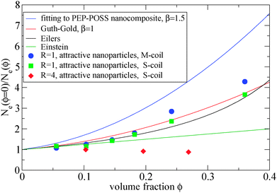Fig. 5 Dependence of N_e(ϕ = 0)/N_e(ϕ) ratio in the frozen particle limit at different nanoparticle loading: (i) fitting of eqn (7) on PEP-POSS nanocomposite⁵⁶ (blue line), (ii) Guth–Gold relation (red line), (iii) Eilers relation (black line), (iv) Einstein relation (green line), (v) attractive nanoparticles: R = 1, M-coil estimator: eqn (4) (circles) (vi) attractive nanoparticles: R = 1 S-coil estimator: eqn (1) (squares) (vii) attractive nanoparticles: R = 4 S-coil estimator: eqn (1) (diamonds). The simulation data are shown for a matrix: N = 200.

3.2.3 Effect of nanoparticle radius on entanglement length N_e. Increasing the radius of the nanoparticles at a constant volume fraction decreases the surface area to volume ratio of the nanoparticles. The effect of the nanoparticle radius on the N_e(ϕ) from our simulations is depicted in Fig. 6. We observe that by increasing the nanoparticle radius to R = 2 we can see a decrease to the discrepancy between the phantom and frozen particle limit. In particular, at ϕ = 25.8%, the S-coil estimator predicts for polymers (N = 200) a value of N_e = 66.1 ± 2.4 in the frozen limit (from M-coil estimator N_e = 64) and N_e = 72.5 ± 1.9 in the phantom limit. Specifically, for nanocomposites with nanoparticles R = 4, the N_e estimators in the phantom and frozen limit are indistinguishable. This implies that nanoparticles of R = 4 do not alter the underlying polymer network for polymer lengths used in our study. Tuteja also found that N_e is unaffected by nanoparticles of R = 5 nm at low nanoparticle loading (ϕ = 8%).^70,71 The interparticle distance of nanoparticles is: ID = D((2/πϕ)^0.333 − 1). For all the nanoparticle volume fractions studied ID < R_g (R_g ≈ 8 for N = 200). In that regime, there is no change in N_e, in the frozen limit, when R_g ≈ D, whereas it changes only if R_g ≫ R (figure in ESI†).

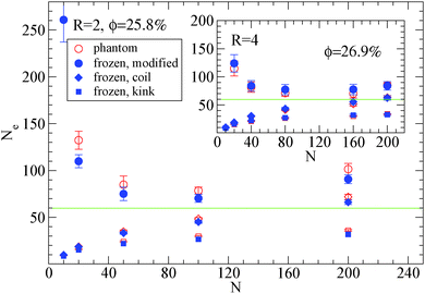Fig. 6 Dependence of N_e using eqn (1), (2) and (3), in the frozen (filled blue symbols) and phantom (open symbols) particle limits of nanocomposites with attractive nanoparticles of R = 2 for nanoparticle loading ϕ = 25.8%: (i) modified S-coil estimator: eqn (3) (circles), (ii) classical S-coil estimator: eqn (1) (diamonds), (iii) classical S-kink estimator: eqn (2) (squares). Inset: Estimators of nanocomposites at ϕ = 26.9% with nanoparticles of R = 4. The green line denotes the N_e for pure polymer melts as extracted by eqn (4).

Also we can observe that in nanocomposites with nanoparticles of R = 2 in a polymer matrix N = 200 (see Fig. 6) the N_e in the phantom limit is enhanced with respect to its polymer melt value. In order to investigate further the polymer path network, we calculated the polymer tube diameter^37,72 and depict it in Fig. 7:

〈α_pp〉 = 〈R_ee²〉/L_pp(ph) (8)

in which L_pp(ph) is extracted in the phantom limit.

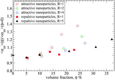Fig. 7 Tube diameter α_pp of polymers (N = 200) at different nanoparticle loading normalized with its value in bulk, obtained from primitive path analysis at the phantom limit for different nanoparticle volume fractions: (i) attractive nanoparticles (R = 1) (open squares), (ii) attractive nanoparticles (R = 2) (diamonds), (iii) attractive nanoparticles (R = 4) (circles) (iv) repulsive nanoparticles (R = 1) (filled squares), (v) repulsive nanoparticles (R = 5) (filled triangles).³⁹ The tube diameter of polymers (N = 200) in bulk is: α_pp = 10.35.

As can be seen in Fig. 7, for attractive small nanoparticles, the tube diameter increases with the nanoparticle loading, whereas for repulsive nanoparticles it remains constant in agreement to the data by Li et al.³⁹ This increase means that such small nanoparticles (R = 1) do alter the polymer network, and the polymers disentangle with nanoparticle loading. This implies that in the case of attractive nanoparticles, the N_e in the phantom limit is increased, as observed in Fig. 3. While the total N_e (in the frozen limit) of the nanocomposite decreases with the nanoparticle loading (see Fig. 4), the polymer–polymer entanglements convert to polymer–nanoparticle entanglements approximately for nanoparticle loading ϕ ≥ 15%. This disentanglement effect does also appear in thin polymer films,⁷³ under cylindrical confinement,^74,75 on a bare flat surface⁷⁶ and on the vicinity of large repulsive spherical nanoparticles at a high nanoparticle loading.³⁹ Furthermore, the polymer chain dynamics can also be affected by the nanoparticle volume fraction. Since by increasing the nanoparticles loading the tube diameter increases, that can enhance the polymer chain's diffusivity. However, direct studies of diffusion remain quite difficult to study the slow reptational dynamics of nanocomposites using molecular dynamics simulations.

4 Conclusions

The polymer density, polymer/polymer and polymer/nanoparticle topological constraints (entanglements) of polymers in melts and nanocomposites containing spherical nanoparticles were investigated by means of molecular dynamics simulations. We applied different N_e(N) estimators for the calculation of the number of entanglements in our systems, and extracted the N-independent entanglement length N_e. We observe that the total N_e decreases even with low volume fraction of small nanoparticles, and significantly for ϕ ≥ 25%. This decrease of N_e, in the nanocomposite, originates from the polymer/nanoparticle entanglements, because the contour length of the primitive path, L_pp, increases with the addition of nanoparticles. In order for polymer nanoparticles entanglements to be formed, the polymers need to be substantially larger than the nanoparticles in order to wrap around them, and in that case the nanoparticles act as topological constraints. Interaction between polymers and nanoparticles does not affect the total entanglement length when there is good nanoparticle dispersion. For the case of attractive small nanoparticles (such as R = 1) the polymer–polymer entanglements decrease (increase of tube diameter) due to the expansion of the polymer chains for ϕ ≥ 15%. This effect on the polymer network is enhanced by the nanoparticle loading. Instead for the case of repulsive nanoparticles the tube diameter remains the same up to ≈ 24% nanoparticle loading in agreement with previous studies.³⁹

Acknowledgements

We thank Prof. M. Kröger for providing us the Z1 algorithm modified for nanocomposites and useful discussions. This research was funded by the EPSRC/NSF Materials Network program EP/5065373/1 (EPSRC: NC, AK) and DMR-1210379 (NSF: KIW, RJC).

References

1. M. Mu, N. Clarke, R. J. Composto and K. I. Winey, Macromolecules, 2009, 42, 7091.
2. A. Karatrantos and N. Clarke, Soft Matter, 2011, 7, 7334.
3. W. S. Tung, V. Bird, R. J. Composto, N. Clarke and K. I. Winey, Macromolecules, 2013, 46, 5345.
4. A. Karatrantos, R. J. Composto, K. I. Winey and N. Clarke, Macromolecules, 2011, 44, 9830.
5. K. Nusser, S. Neueder, G. J. Schneider, M. Meyer, W. Pyckhout-Hintzen, L. Willner, A. Radulescu and D. Richter, Macromolecules, 2010, 43, 9837.
6. G. J. Schneider, K. Nusser, L. Willner, P. Falus and D. Richter, Macromolecules, 2011, 44, 5857.
7. S. Gam, J. S. Meth, S. G. Zane, C. Chi, B. A. Wood, M. E. Seitz, K. I. Winey, N. Clarke and R. J. Composto, Macromolecules, 2011, 44, 3494.
8. S. Gam, J. S. Meth, S. G. Zane, C. Chi, B. A. Wood, K. I. Winey, N. Clarke and R. J. Composto, Soft Matter, 2012, 8, 6512.
9. C. C. Lin, S. Gam, J. S. Meth, N. Clarke and K. I. Winey, Macromolecules, 2013, 46, 4502.
10. S. Sen, Y. Xie, S. K. Kumar, H. Yang, A. Bansal, D. L. Ho, L. Hall, J. B. Hooper and K. S. Schweizer, Phys. Rev. Lett., 2007, 98, 128302.
11. M. K. Crawford, R. J. Smalley, G. Cohen, B. Hogan, B. Wood, S. K. Kumar, Y. B. Melnichenko, L. He, W. Guise and B. Hammouda, Phys. Rev. Lett., 2013, 110, 196001.
12. A. Tuteja, P. M. Duxbury and M. E. Mackay, Phys. Rev. Lett., 2008, 100, 077801.
13. A. I. Nakatani, W. Chen, R. G. Schmidt, G. V. Gordon and C. C. Han, Polymer, 2001, 42, 3713.
14. A. Karatrantos, N. Clarke, R. J. Composto and K. I. Winey, Soft Matter, 2015, 11, 382.
15. A. L. Frischknecht, E. S. McGarrity and M. E. Mackay, J. Chem. Phys., 2010, 132, 204901.
16. P. S. Stephanou, J. Chem. Phys., 2015, 142, 064901.
17. N. Jouault, F. Dalmas, S. Said, E. Di Cola, R. Schweins, J. Jestin and F. Boue, Macromolecules, 2010, 43, 9881.
18. R. A. Riggleman, G. Toepperwein, G. J. Papakonstantopoulos, J.-L. Barrat and J. J. de Pablo, J. Chem. Phys., 2009, 130, 244903.
19. Q. W. Yuan, A. Kloczkowski, J. E. Mark and M. A. Sharaf, J. Polym. Sci., Polym. Phys. Ed., 1996, 34, 1647.
20. D. Gersappe, Phys. Rev. Lett., 2002, 89, 058301.
21. J. Liu, Y. Wu, J. Shen, Y. Gao, L. Zhang and D. Cao, Phys. Chem. Chem. Phys., 2011, 13, 13058.
22. A. Kutvonen, G. Rossi and T. Ala-Nissila, Phys. Rev. E: Stat., Nonlinear, Soft Matter Phys., 2012, 85, 041803.
23. E. Masnada, S. Merabia, M. Couty and J. L. Barrat, Soft Matter, 2013, 9, 10532.
24. A. E. Likhtman, Macromolecules, 2005, 38, 6128.
25. N. Jouault, F. Dalmas, F. Boue and J. Jestin, Polymer, 2012, 53, 761.
26. G. D. Hattemer and G. Arya, Macromolecules, 2015, 48, 1240.
27. A. Karatrantos, N. Clarke and M. Kröger, Polym. Rev., 2015 DOI:10.1080/15583724.2015.1090450.
28. A. Kutvonen, G. Rossi, S. R. Puisto, N. K. J. Rostedt and T. Ala-Nissila, J. Chem. Phys., 2012, 137, 214901.
29. E. Jaber, H. Luo, W. Li and D. Gersappe, Soft Matter, 2011, 7, 3852.
30. V. Padmanabhan, J. Chem. Phys., 2013, 139, 144904.
31. A. A. Gavrilov, A. V. Chertovich, P. G. Khalatur and A. Khokhlov, Macromolecules, 2014, 47, 5400.
32. Y. Li, Polymer, 2011, 52, 2310.
33. Y. Li, M. Kröger and W. K. Liu, Macromolecules, 2012, 45, 2099.
34. A. Karatrantos, N. Clarke, R. J. Composto and K. I. Winey, Soft Matter, 2013, 9, 3877.
35. A. Karatrantos, R. J. Composto, K. I. Winey and N. Clarke, IOP Conf. Ser.: Mater. Sci. Eng., 2012, 40, 012027.
36. G. N. Toepperwein, N. C. Karayiannis, R. A. Riggleman, M. Kröger and J. J. de Pablo, Macromolecules, 2011, 44, 1034.
37. L. Cai, S. Panyukov and M. Rubinstein, Macromolecules, 2011, 44, 7853.
38. A. Karatrantos, R. J. Composto, K. I. Winey, M. Kröger and N. Clarke, Macromolecules, 2012, 45, 7274.
39. Y. Li, M. Kröger and W. K. Liu, Phys. Rev. Lett., 2012, 109, 118001.
40. Y. Termonia, Polymer, 2010, 51, 4448.
41. Y. Termonia, J. Polym. Sci., Part B: Polym. Phys., 2010, 48, 687.
42. M. E. Mackay, T. T. Dao, A. Tuteja, D. L. Ho and H.-C. Horn, Nat. Mater., 2003, 2, 762.
43. C. Ohrt, T. Koschine, K. Rätzke, F. Faupel, L. Willner and G. J. Schneider, Macromolecules, 2014, 55, 143.
44. M. Kröger, Comput. Phys. Commun., 2005, 168, 209.
45. R. Everaers, S. K. Sukumaran, G. S. Grest, C. Svaneborg, A. Sivasubramanian and K. Kremer, Science, 2004, 303, 823.
46. S. Shanbhag and M. Kröger, Macromolecules, 2007, 40, 2897.
47. R. S. Hoy, K. Foteinopoulou and M. Kröger, Phys. Rev. E: Stat., Nonlinear, Soft Matter Phys., 2009, 80, 031803.
48. N. C. Karayiannis and M. Kröger, Int. J. Mol. Sci., 2009, 10, 5054.
49. M. Doi and S. F. Edwards, The Theory of Polymer Dynamics, Clarendon Press, Oxford, 1986.
50. P. J. Flory, Statistical Mechanics of Chain Molecules, Hanser, Munchen, 1989.
51. A. E. Likhtman, S. K. Sukumaran and J. Ramirez, Macromolecules, 2007, 40, 6748.
52. M. Bulacu and E. van der Giessen, J. Chem. Phys., 2005, 123, 114901.
53. K. Kremer and G. S. Grest, J. Chem. Phys., 1990, 92, 5057.
54. M. Putz, K. Kremer and G. S. Grest, Europhys. Lett., 2000, 49, 735.
55. N. Uchida, G. s. Grest and R. Everaers, J. Chem. Phys., 2008, 128, 044902.
56. K. Nusser, G. I. Schneider, W. Pyckhout-Hintzen and D. Richter, Macromolecules, 2011, 44, 7820.
57. J. T. Kalathi, G. S. Grest and S. K. Kumar, Phys. Rev. Lett., 2012, 109, 198301.
58. D. Meng, S. K. Kumar, S. Cheng and G. S. Grest, Soft Matter, 2013, 9, 5417.
59. T. K. Patra and J. K. Singh, J. Chem. Phys., 2013, 138, 144901.
60. S. K. Sukumaran, G. S. Grest, K. Kremer and R. Everaers, J. Polym. Sci., Part B: Polym. Phys., 2005, 43, 917.
61. R. Everaers, Phys. Rev. E: Stat., Nonlinear, Soft Matter Phys., 2012, 86, 022801.
62. K. Nusser, G. J. Schneider and D. Richter, Macromolecules, 2013, 46, 6263.
63. H. Eggers and P. Schuemmer, Rubber Chem. Technol., 1996, 69, 253.
64. G. Heinrich, M. Kluppel and T. A. Vilgis, Curr. Opin. Solid State Mater. Sci., 2002, 6, 195.
65. E. T. Kopesky, T. S. Haddad, G. H. McKinley and R. E. Cohen, Polymer, 2005, 46, 4743.
66. A. Einstein, Ann. Phys., 1906, 19, 289.
67. H. J. Smallwood, J. Appl. Phys., 1944, 15, 758.
68. E. Guth and O. Gold, Phys. Rev., 1938, 53, 322.
69. V. H. Eilers, Kolloid-Z., 1941, 3, 313.
70. A. Tuteja and M. E. Mackay, Nano Lett., 2007, 7, 1276.
71. R. Mangal, S. Srivastava and L. A. Archer, Nat. Commun., 2015, 6, 7198.
72. F. Lahmar, C. Tzoumanekas, D. N. Theodorou and B. Rousseau, Macromolecules, 2009, 42, 7485.
73. H. Meyer, T. Kreer, A. Cavallo, J. P. Wittmer and J. Baschnagel, Eur. Phys. J.: Spec. Top., 2007, 141, 167.
74. D. Sussman, W. S. Tung, K. Winey, K. S. Schweizer and R. A. Riggleman, Macromolecules, 2014, 47, 6462.
75. W. S. Tung, R. J. Composto, R. A. Riggleman and K. Winey, Macromolecules, 2015, 48, 2324.
76. M. Vladkov and J. L. Barrat, Macromolecules, 2007, 40, 3797.

---

Footnote

† Electronic supplementary information (ESI) available. See DOI: 10.1039/c5sm02010g

---