Regional feature extraction of various fishes based on chemical and microbial variable selection using machine learning

Abstract

We introduce a method for extracting regional and habitat features of various fish species based on chemical and microbial correlations that incorporate integrated analysis and a variable selection approach. We characterized 24 fish species from two marine regions in Japan, in terms of the metabolic and inorganic profiles of muscle and gut contents, as well as gut microbes. Using machine learning, the integrated analysis based on the metabolic, inorganic, and microbial profiles of muscle and gut contents allows the characterization of both the fish species and habitat regions. The results revealed that the fish muscle tissue profile provides high-value data for evaluating ecosystems and discriminating fish populations based on species and regions. To visualize the regionality and habitat, we developed a method to efficiently extract the most important variables using the machine learning approach, followed by correlation analysis of variations in muscle and gut content profiles. The correlation networks enabled efficient visualization of marine ecosystems in the Tohoku and Kanto regions of Japan. This method should be useful for evaluating fish habitats and elucidating associated environmental chemical networks.

---

Introduction

Living organisms are essential for maintaining the ecosystems of the Earth.¹ Biological and physiochemical cycles form ecological networks through their complex and diverse interactions.² These ecological networks are influenced not only by biological interactions such as predator–prey relationships, but also significantly by abiotic and environmental factors.³ Therefore, abiotic factors such as chemicals and nutrients should be comprehensively analyzed when evaluating ecological networks.⁴

Fish are an important aquatic resource and play a vital role in aquatic ecosystems.⁵ Since fishes incorporate inorganic nutrients and microbial communities from their environments into their bodies, it is presumed that geography can influence environmental factors, which ultimately affect the physiology and ecology of fishes.⁶ Our previous studies evaluated the sources of environmental variation that maintains fish populations in coastal and estuarine environments^7,8 and revealed the geographical differences in organic and inorganic substances and microbial communities in coastal and estuarine sediments⁹ and coastal terrestrial soils¹⁰ in the Tohoku and Kanto regions of Japan. These chemical and microbial profiles of fish bodies were strongly influenced by their environment, suggesting that geographical difference may influence regional chemical profiles.

Many analytical methods have been used to evaluate the interaction between fish and the environment. For example, to evaluate the influence of environmental chemicals in fish habitats, exposure experiments were performed using laboratory animals, such as Japanese killifish, fathead minnow,^11–13 and other fish species.^13–15 In these analyses, many analytical techniques were crucial for evaluating the relationships between fish metabolism/physiology/ecology and their environments, e.g., gene expression analysis by transcriptome sequencing,^16,17 phylogenetic analysis,^18–20 microbiota analysis in the gut^6,21,22 and sediment,^9,23 and metabolomics.^24–28 In particular, the nuclear magnetic resonance (NMR)-based metabolomic technique offers a high throughput, easy sample preparation, and inter-institution convertibility.^29–33 Thus, it has been used extensively for analyzing biological and environmental systems. Examples include the influence of frozen storage on fish organs,³⁴ exposure of fishes to sewage,³⁵ polycyclic aromatic hydrocarbon exposure,¹⁶ organophosphorus toxin exposure,³⁶ and analysis of fish eggs³⁷ and fish oils.³⁸ However, most of these studies used only one or two species and a single analytical method, and there is only limited knowledge about how this technique applies to a wider diversity of fish species. In order to evaluate environmental conditions and ecosystems, it seems necessary to evaluate responsiveness based on complex chemical and biological interactions among a diverse array of fish species.

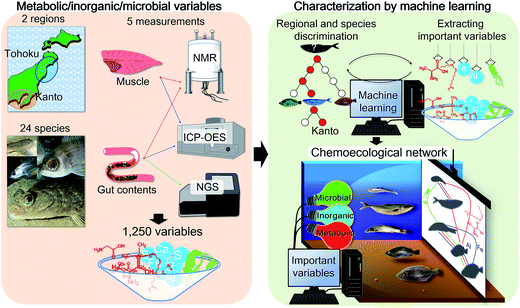
We have previously proposed that the host chemical³⁹ and gut microbial profiles of fish are strongly influenced by their food source,²² suggesting that these host and symbiotic profiles could provide insights into the habitats the samples were collected from. From this perspective, we have developed visualization methods to examine the chemical and microbial correlations in aquatic environments (e.g. paddy fields,⁴⁰ coastal and estuarine sediments,⁹ coastal algae,^41,42 and coastal and estuarine fishes^43,44), and identified many variables related to metabolites, inorganic substances, and related information on microbes. Since these variables include both changeable and stable ones, developing a variable selection and visualization method would be important for evaluating environmental conditions. In this study, we advanced our analytical approach by developing a procedure to select important (key) variables using a machine learning approach, based on discrimination between key variables and background noise (Fig. 1). The developed technique was applied to the fish samples of different species, ecological conditions, and coastal environments (Tohoku and Kanto regions in Japan). Furthermore, an evaluation method for visualizing fish chemical and microbial networks was developed based on important selection variables. The networks capture interactive associations among organic compounds, inorganic compounds, and microbial communities in fish habitats (environments) that contribute to the environmental maintenance of ecological homeostasis.

Fig. 1 Conceptual diagram illustrating correlation network analysis of regional fish habitats using variations in chemical and microbial signatures. We characterized metabolic and inorganic profiles of muscle and gut contents and gut microbes for 24 fish species that inhabit two marine regions of Japan using nuclear magnetic resonance (NMR), inductively coupled plasma-optical emission spectrometry (ICP-OES), and next-generation sequencing (NGS). For the visualization of the ecosystems, we developed a method to efficiently extract the most important variables from all variables, using a machine learning approach. All the figures were drawn by Taiga Asakura, using R platform 3.3.3, Gephi 8.0, Adobe Illustrator CS6 and Microsoft Powerpoint 2013. All photographs were taken by Taiga Asakura.

Experimental

Sample collection and preparation

Fish samples were obtained from the Kanto and Tohoku regions in Japan from 2011 to 2016. Due to different latitudes, these geographically distant regions (see maps in Fig. S1†) differ in air and water temperatures. The shape of the ocean floor and tidal flow along the coast are also very different. The collected fish species, number of samples, sampling sites, and habitats (depth and distance from the coast) are listed in Table S1.† The average sample size of each fish species was 20 for muscle tissues and 10 for gut contents. The fish samples are identified by abbreviations and labels as shown in Fig. S2 and Table S1.† Photos of the fish species from previous phylogenetic studies^18–20 are also shown in Fig. S2.† The muscles and whole gut contents of fish were freeze-dried and powderized (10 min for NMR extraction and 1 min for DNA extraction) using an Automill machine (Tokken, Inc., Chiba, Japan) for metabolic, elemental, and microbial community analyses.

Ethics statement

No specific permission was required at any of the sampling places because fish catching at public places is not against the law of Japan. All experiments were conducted according to the principles and procedures of the RIKEN Animal Care and Use Committee approved by the Institutional Regulation for Animal Experiments and Fundamental Guidelines for Proper Conduct of Animal Experiment and Related Activities in Academic Research Institutions under the jurisdiction of the Ministry of Education, Culture, Sports, Science and Technology, Japan. Since anesthetic chemicals such as 2-phenoxyethanol may influence metabolic profiling, ice tightening was quickly performed on all fishes used in our study similar to other fishery and aquaculture products at the time of sampling.

NMR measurements

The metabolic profiles of fish muscles and gut contents were measured using an NMR system (AVANCE II 700 spectrometer, Bruker BioSpin GmbH, Rheinstetten, Germany). Powdered samples (10 mg) were extracted using methanol (600 μL) according to the procedure outlined in a previous study.²² One-dimensional (1D) ¹H NMR and two-dimensional ¹H–¹³C heteronuclear single quantum coherence (HSQC) spectra were obtained using the same procedures and parameters as described in this ref. 22. The NMR signals were annotated using SpinAssign^45,46 and the Biological Magnetic Resonance Bank.⁴⁷

Inorganic elements in fish samples

The elemental profiles of fish muscles (10 mg) and gut contents (10 mg) were measured using inductively coupled plasma-optical emission spectrometry (ICP-OES, SPS5510, SII NanoTechnology, Chiba, Japan) by following methods used in previous study.⁴⁸

Microbial community analysis of fish gut contents

The microbial community profiles of fish gut contents were measured using a MiSeq sequencer (Illumina, San Diego, CA). Microbial DNAs were extracted according to a reported protocol with slight modifications.⁴⁹ The microbial DNAs were amplified by polymerase chain reaction (PCR) with target universal primers for bacterial 16S rRNA gene, according to previous reports.⁵⁰ The PCR products were sequenced on the MiSeq sequencer by following the manufacturer's instructions, followed by data analysis using QIIME software (http://qiime.org/).⁵¹ The obtained sequences were expressed as operational taxonomic units, whereas results showing more than 97% similarity were regarded to be from the same taxonomic group.

Statistical analyses

The NMR spectra were processed into a data matrix using a peak-picking algorithm based on the region of interest (ROI) using rNMR software.⁵² The ROIs comprised of information about peak intensities and chemical shifts indicative of the region. Based on different NMR peak intensities among the substances, the data matrix was normalized by constant sum in order to avoid their influence on the correlation analysis. The ICP-OES data utilized the intensity of the wavelength of each element, whereas the microbial data utilized the percentage of the total read number assigned to the taxonomic family level for statistical analysis. The NMR, ICP-OES, and MiSeq data from the same individual fish were used to create a single integrated matrix. Principal component analysis (PCA) and random forest (RF) approach were implemented in the R language using the “randomForest” package.^53,54 RF is an algorithm for classification and regression modeling using hundreds of decision trees, and it is frequently employed in recent biomarker discovery and structure prediction studies.^55,56 For classification modeling, the species and geographical locations of fishes were used as dependent variables; all metabolic and elemental data of the fish samples were chosen as the training data set, except the data of one fish sample which were used as test data to validate the consistency of the models (i.e., the leave-one-out cross-validation procedure). Modeling with RF and the corresponding calculations of the test data were repeatedly performed on all individual fish species based on randomly extracted learning data. The calculation results and their importance values are given as mean values. The identified variables were arranged in descending order, based on the importance values obtained when creating the classification model. Variable selections were performed based on model accuracies. In this evaluation of variables, 10% of the data set was used as the test data, and the obtained accuracy was averaged over 100 routines. Based on the selected variables, Spearman's rank correlation coefficients were calculated and averaged for each fish species. The obtained average correlation coefficient cut-off threshold value was 0.5, the fish species were drawn as nodes, and correlation coefficients of 0.5 or higher were drawn as edges with Gephi (http://gephi.org), according to previous studies.⁴¹

Results and discussion

Metabolic/inorganic/microbial characterization using an unsupervised approach

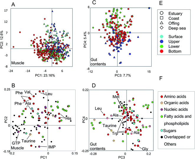
The metabolic variability of the methanol fractions from fish muscle and gut contents was evaluated using NMR spectra, with metabolite annotations provided by HSQC NMR in combination with the SpinAssign program, by referencing previous reports,^7,22,42 see Fig. S3 and Table S2.† The HSQC NMR spectral data included signals from amino acids, organic acids, nucleic acids, fatty acids, and sugars. The gut contents comprised more diverse materials than the muscle tissue.

The metabolic variability of the muscle tissue and gut contents was characterized by the fish habitat and species, based on the principal component (PC) scores using PCA (Fig. 2). From Fig. 2A and B, it can be seen that the muscle metabolic profiles are clearly indicated by PC scores, which reflect the characteristics of each species and its ecology (depth and distance from the coast). The metabolic profiles of the gut contents convey the same characteristics, but less so for the ecology than the muscle tissue profiles because the ecological characteristics were observed in not PCs 1 and 2 but PCs 3 and 4 (Fig. 2C and D). Several inorganic compounds were detected in the muscle and gut contents of all fish species, i.e., their occurrence was not species-specific (Fig. S4†). The exceptions were Fe and Al, which were abundant in the gut contents of estuarine and coastal fishes that are mainly omnivorous, compared to the contents of a predatory fish collected from the same habitats. Since Fe and Al are abundant in the estuarine sediments,⁹ our results suggest that habitats and food choice both affect the abundance of these two elements.

Fig. 2 PCA results of fish muscle and gut contents based on ¹H-NMR profiles. Metabolic profiles of muscle tissue (A and B, n = 476, k = 117) and gut contents (C and D, n = 257, k = 121) were evaluated using PCA score plots (A and C) and loading plots (B and D). E: symbols on PCA score plots express different areas and depths (denoted by shape and color, respectively). F: colors on PCA loading plots indicate the type of metabolites.

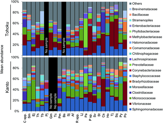
The microbial community profiles indicated that Micrococcaceae and Vibrionaceae were abundantly present in the Kanto and Tohoku regions, respectively (Fig. 3). The Shannon diversity index (at the genus level of microbiota profiles) had been used to evaluate the microbial diversity in fish guts, fish feces, human feces,⁵⁷ and coastal and shallow sea sediments.⁹ For a plot of these factors against the fish length across various marine environments, see Fig. S5A.† The diversity of microbial communities in fish guts varied more widely compared to that in human feces (Fig. S5A†). Interestingly, the diversity of microbes in fish guts was negatively correlated with the fish body length and not associated with fish habitats (Fig. S5†). In particular, Photobacterium sp. tends to be the predominant species in the guts of larger fish. Sphingomonas sp. and Renibacterium sp. tend to have a similar occupancy, and their total abundance was often significantly higher in smaller fishes (Fig. S5B†). We suggest that fish gut microbial communities change in composition as the fish grows, possibly due to changes in feeding habits over time. Moreover, we propose that not optimization of the microbial community may be found in relatively small fish, based on the higher microbial diversity than that found in larger, predatory fish.

Fig. 3 Microbial community profiles in each fish species and sampled region. The values indicate the mean of relative abundance for each fish species in Tohoku (upper part) and Kanto (lower part) regions.

Discrimination modeling of ecosystems from integrated fish metabolic/inorganic/microbial profiles by machine learning

In order to characterize the integrated metabolic/inorganic/microbial profiles as ecosystems in the Kanto and Tohoku regions, a congregative evaluation was performed using the RF model. For RF modeling, decision mtry (number of variables randomly sampled as candidates at each split) and number of trees were set to the minimum number needed to achieve the highest accuracy rate (Fig. S6†). The results of the leave-one-out cross-validation procedure are shown in Table S3† and integrated as shown in Fig. 4. The average accuracy rate was 72.3% at both the species and regional sampling levels, 84.7% at the species level, 89.6% at the family level, and 90.6% at the order level. The predictions for Engraulis japonicus, Trachurus japonicus, and Seriola quinqueradiata were 100% accurate at the regional level, indicating that it was easy to distinguish the collection regions (Kanto vs. Tohoku) using these species. Most of the other fish species could be discriminated at a rate of 80%. In contrast, Gadus macrocephalus and Theragra chalcogramma had low rates of species-level accuracy, whereas the family level (Gadidae) was accurately discriminated. We attribute the low accuracy to each species being close, genetically and ecologically.¹⁸ Thus, our approach based on metabolic profiling of gut microbes allowed the differentiation of sampling areas and geographical origins from the mixtures (models) of numerous fish species.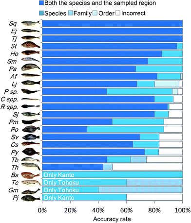

Fig. 4 Discriminant model from RF analysis based on integrated metabolic/inorganic/microbial profiles. The discrimination accuracy of the RF model was described using cross-validation (Table S3†). The five legends, from top to bottom and left to right, denote the ratios of (i) correct discriminations for both the species and sampled region, (ii) correct for the species but incorrect for the sampled region, (iii) correct at the family level but incorrect at the species level, (iv) correct at the order level but incorrect at the family level, and (v) incorrect for both the taxonomy and the sampled region. For the species abbreviations see Fig. S2.†

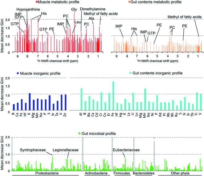
When we calculated the Gini impurity,^58,59 we found that the models were best explained by the NMR-based host metabolic profiles,^60,61 followed by the inorganic elements in the fish gut contents, and least by the gut microbial community. The most important variables identified for the discrimination model were the metabolites of the muscle tissue such as glycine, histidine, hypoxanthine, and taurine (Fig. 5), suggesting that our approach could determine the most important metabolites for characterizing and discriminating phylogenetic and geographical differences in a non-linear manner. In particular, glycine, histidine, and inosine 5′-monophosphate (IMP) robustly reflected the sampled regions and species. In contrast, the organic matter profiles of the gut content were not strongly indicative, and so we concluded that the fish's diet had little effect on the regional metabolic characteristics.⁶² Moreover, the gut inorganic profiles were relatively more important, suggesting that they were affected by minerals derived from marine sediments.⁶³

Fig. 5 Variation in the importance of models based on the mean decrease in the Gini impurity coefficient. The vertical axis (mean decrease Gini) describes the degree of importance obtained from the RF model. The variables of the metabolite profiles are expressed on the basis of chemical shifts. The inorganic and microbial profiles are represented by the elements and family of microbes, respectively. PC: phosphatidylcholine, PE: phosphatidylethanolamine.

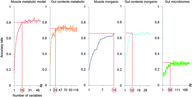
The exploration of important variables using the RF procedure is shown in Fig. 6. In most models, the accuracy stopped rising before all the variables were examined. Thus, the smallest number of variables that can maintain a high accuracy for the model were regarded as the most important explanatory variables.

Fig. 6 Selection of the most important variables for each profile. Variable numbers arranged in the descending order of the importance index are on the horizontal axis, and the average accuracy is on the vertical axis. The number of variables with the highest importance is indicated by the red line.

The muscle metabolite profile model provided the highest accuracy, followed by the gut content metabolite model, the gut content inorganic model, the muscle inorganic model, and the gut microbiome model, in this order. The important variables for each profile are listed in Table S4.† To compare these models with an unsupervised analysis, PCA was performed using the same samples and the results are shown in Fig. 2A by using the important variables. In the obtained results (Fig. S7†), The differences among habitats appear more clearly. A U test was performed to quantitatively determine the difference between each species pair (Fig. S8†). Because there were multiple comparisons, significant differences were defined by the Bonferroni procedure (with 276 examinations, the significant p-values were less than 0.05/276). The p-value of each species showed a larger number of significant differences using the most important explanatory variables selected as shown in Fig. 6, compared to that using all the variables. Hence, our results indicate that the selection of important variables is effective for evaluating differences among the species and their ecology. Moreover, from the high importance and accuracy of the obtained muscle metabolite profiles, NMR is effective for discriminating the species and regions.

Correlation network analysis based on selected chemical and microbial variables

The raw data were used to visualize relationships among the fish species. The important metabolic/inorganic/microbial variables for the muscle and gut contents were assessed through positive correlations obtained using Spearman's rank correlation coefficient (Table S5†). The correlations were expressed by nodes and edges; the nodes of the fish samples were connected with each other using lines when their correlation was >+0.5 (Fig. 7 and S9†).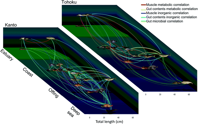

Fig. 7 Chemical and microbial diagrams based on integrated correlation network analysis. The line thickness corresponds to the correlation coefficients of the respective measurement conditions. The horizontal axis depicts the average size of the fishes and depth, and the vertical axis represents the habitats. For detailed data refer Fig. S10 and Table S5.† All photographs were taken by T. Asakura.

Fig. S9† was derived with the ForceAtlas algorithm of Gephi. The muscle metabolite profile networks always connected the bottom-dwelling group and the epipelagic group. Gadus macrocephalus and Theragra chalcogramma (closely linked genetically and ecologically) appeared connected in most networks. On the other hand, although Seriola quinqueradiata and Scomber japonicus are from different families, they were connected in many networks for both the Kanto and Tohoku region samples, probably because of their similar habits. A summary of the resulting networks is presented in Fig. 7, where the locations of nodes and edges are based on the type of sampled habitat and sample size. For instance, some fishes, such as Trachurus japonicus and Clupeiformes exhibited relationships that differed from the other fish species in the Kanto and Tohoku regions (Fig. 7 and S9†). Trachurus collected in Tohoku was correlated with epipelagic fish like Seriola, which live in the off-shore zones of the Tohoku region, while Trachurus collected in Kanto was correlated with bottom-dwelling fish like Pleuronectes. Because Trachurus is known to live in two types of habitats (bay and off-shore),⁶² we suspect that the specimens collected in the Tohoku region are associated with the off-shore habitats, while those collected in Kanto are associated with the bay habitats. We further speculate that the metabolic networks describing the Kanto and Tohoku regions reflect different ecosystems and food webs. In addition, the size and feeding habits of Seriola and sardines differ rather markedly between the two regions. For example, in networks, Seriola collected in Kanto was most strongly correlated with Engraulis, whereas Seriola collected in Tohoku was correlated with Sardinops. These correlations among the networks indicate predator–prey relationships. Considering such metabolic correlations among networks, we surmise that species in a predator-prey system share essential amino acids and essential fatty acids as metabolites in muscle tissue. Obviously, the muscle and gut contents in the inorganic and microbial networks of the Kanto region must have been connected over a wide range (Fig. S9D and S9E†). Compared to the Tohoku region, the Kanto region has a more complex and diverse coastal morphology, which is supported by the strong correlation between the fish and sediment compositions. In sum, examining the interrelationships among fish metabolites and elements is a new way to monitor environmental quality.⁹

This study focused on evaluating and characterizing the regionality and habitat based on the metabolic, inorganic, and microbial diversity among various fish species in two marine ecosystems in Japan. By selecting and comparing important variables from an integrated profile it is revealed that it is possible to efficiently extract ecological relationships among the species and regions. We demonstrated that the muscle metabolic profile obtained using the NMR technique can strongly discriminate between fish species and habitats. The integrated data allow one to differentiate between different species and sampled areas by using a machine learning (RF) model. Therefore, the combination of NMR profiling with machine learning can have potential applications in characterizing fishery production regions, as well as evaluating fishery management and sustainability in aquaculture. Based on the correlation analyses of the metabolic, inorganic, and microbial profiles, we could visualize fish habitats by using chemical and microbial network analysis in the two regions. This approach is useful for elucidating environmental chemical networks, because the samples are relatively easy to prepare, the data are reproducible and stable, and the approach can reveal important metabolite structures relative to various marine environments.

Author contribution statement

T. Asakura, Y. Date, and J. Kikuchi wrote the main manuscript text and prepared the figures. K. Sakata contributed to the technical experiments and prepared figures. All authors reviewed the manuscript.

Conflicts of interest

The authors declare no competing financial interests.

Acknowledgements

We thank S. Moriya, T. Kato, and T. Ogura for supporting the microbial analysis; and M. Akama, T. Shimizu, A. Takada, and Y. Otaka for technical assistance. This work was supported in part by J.S.P.S. and the Fisheries Agency, and also supported by Agriculture, Forestry and Fisheries Council, Japan.

References

1. P. Neubauer, O. P. Jensen, J. A. Hutchings and J. K. Baum, Science, 2013, 340, 347–349.
2. W. W. L. Cheung, J. L. Sarmiento, J. Dunne, T. L. Frolicher, V. W. Y. Lam, M. L. D. Palomares, R. Watson and D. Pauly, Nat. Clim. Change, 2013, 3, 254–258.
3. B. Worm, Proc. Natl. Acad. Sci. U. S. A., 2015, 112, 11752–11753.
4. J. R. Jambeck, R. Geyer, C. Wilcox, T. R. Siegler, M. Perryman, A. Andrady, R. Narayan and K. L. Law, Science, 2015, 347, 768–771.
5. B. S. Halpern, C. Longo, D. Hardy, K. L. McLeod, J. F. Samhouri, S. K. Katona, K. Kleisner, S. E. Lester, J. O'Leary, M. Ranelletti, A. A. Rosenberg, C. Scarborough, E. R. Selig, B. D. Best, D. R. Brumbaugh, F. S. Chapin, L. B. Crowder, K. L. Daly, S. C. Doney, C. Elfes, M. J. Fogarty, S. D. Gaines, K. I. Jacobsen, L. B. Karrer, H. M. Leslie, E. Neeley, D. Pauly, S. Polasky, B. Ris, K. St Martin, G. S. Stone, U. R. Sumaila and D. Zeller, Nature, 2012, 488, 615–620.
6. L. Ye, J. Amberg, D. Chapman, M. Gaikowski and W. T. Liu, ISME J., 2014, 8, 541–551.
7. S. Yoshida, Y. Date, M. Akama and J. Kikuchi, Sci. Rep., 2014, 4, 7005.
8. Y. Date and J. Kikuchi, Anal. Chem., 2018, 90, 1805–1810.
9. T. Asakura, Y. Date and J. Kikuchi, Anal. Chem., 2014, 86, 5425–5432.
10. T. Ogura, Y. Date, Y. Tsuboi and J. Kikuchi, ACS Chem. Biol., 2015, 10, 1908–1915.
11. T. W. Collette, Q. Teng, K. M. Jensen, M. D. Kahl, E. A. Makynen, E. J. Durhan, D. L. Villeneuve, D. Martinovic-Weigelt, G. T. Ankley and D. R. Ekman, Environ. Sci. Technol., 2010, 44, 6881–6886.
12. J. M. Davis, T. W. Collette, D. L. Villeneuve, J. E. Cavallin, Q. Teng, K. M. Jensen, M. D. Kahl, J. M. Mayasich, G. T. Ankley and D. R. Ekman, Environ. Sci. Technol., 2013, 47, 10628–10636.
13. D. R. Ekman, D. M. Skelton, J. M. Davis, D. L. Villeneuve, J. E. Cavallin, A. Schroeder, K. M. Jensen, G. T. Ankley and T. W. Collette, Environ. Sci. Technol., 2015, 49, 3091–3100.
14. G. Nestor, J. Bankefors, C. Schlechtriem, E. Brannas, J. Pickova and C. Sandstrom, J. Agric. Food Chem., 2010, 58, 10799–10803.
15. L. Wagner, S. Trattner, J. Pickova, P. Gomez-Requeni and A. A. Moazzami, Food Chem., 2014, 147, 98–105.
16. T. D. Williams, H. Wu, E. M. Santos, J. Ball, I. Katsiadaki, M. M. Brown, P. Baker, F. Ortega, F. Falciani, J. A. Craft, C. R. Tyler, J. K. Chipman and M. R. Viant, Environ. Sci. Technol., 2009, 43, 6341–6348.
17. E. M. Santos, J. S. Ball, T. D. Williams, H. F. Wu, F. Ortega, R. Van Aerle, I. Katsiadaki, F. Falciani, M. R. Viant, J. K. Chipman and C. R. Tyler, Environ. Sci. Technol., 2010, 44, 820–826.
18. T. J. Near, A. Dornburg, R. I. Eytan, B. P. Keck, W. L. Smith, K. L. Kuhn, J. A. Moore, S. A. Price, F. T. Burbrink, M. Friedman and P. C. Wainwright, Proc. Natl. Acad. Sci. U. S. A., 2013, 110, 12738–12743.
19. M. Miya, H. Takeshima, H. Endo, N. B. Ishiguro, J. G. Inoue, T. Mukai, T. P. Satoh, M. Yamaguchi, A. Kawaguchi, K. Mabuchi, S. M. Shirai and M. Nishida, Mol. Phylogenet. Evol., 2003, 26, 121–138.
20. S. Lavoue, M. Miya, K. Saitoh, N. B. Ishiguro and M. Nishida, Mol. Phylogenet. Evol., 2007, 43, 1096–1105.
21. S. Smriga, S. A. Sandin and F. Azam, FEMS Microbiol. Ecol., 2010, 73, 31–42.
22. T. Asakura, K. Sakata, S. Yoshida, Y. Date and J. Kikuchi, PeerJ, 2014, 2, e550.
23. A. Bissett, J. Bowman and C. Burke, FEMS Microbiol. Ecol., 2006, 55, 48–56.
24. G. Shen, Y. Huang, J. Dong, X. Wang, K. K. Cheng, J. Feng, J. Xu and J. Ye, J. Agric. Food Chem., 2018, 66, 368–377.
25. R. Melis, R. Sanna, A. Braca, E. Bonaglini, R. Cappuccinelli, H. Slawski, T. Roggio, S. Uzzau and R. Anedda, Comp. Biochem. Physiol., Part A: Mol. Integr. Physiol., 2017, 204, 129–136.
26. K. Cheng, E. Mullner, A. A. Moazzami, H. Carlberg, E. Brannas and J. Pickova, J. Agric. Food Chem., 2017, 65, 5083–5090.
27. F. Casu, A. M. Watson, J. Yost, J. W. Leffler, T. G. Gaylord, F. T. Barrows, P. A. Sandifer, M. R. Denson and D. W. Bearden, J. Proteome Res., 2017, 16, 2481–2494.
28. T. Cappello, F. Brandao, S. Guilherme, M. A. Santos, M. Maisano, A. Mauceri, J. Canario, M. Pacheco and P. Pereira, Sci. Total Environ., 2016, 548–549, 13–24.
29. A. D. Southam, J. M. Easton, G. D. Stentiford, C. Ludwig, T. N. Arvanitis and M. R. Viant, J. Proteome Res., 2008, 7, 5277–5285.
30. H. Motegi, Y. Tsuboi, A. Saga, T. Kagami, M. Inoue, H. Toki, O. Minowa, T. Noda and J. Kikuchi, Sci. Rep., 2015, 5, 15710.
31. J. Kikuchi, Y. Tsuboi, K. Komatsu, M. Gomi, E. Chikayama and Y. Date, Anal. Chem., 2016, 88, 659–665.
32. J. Kikuchi, K. Ito and Y. Date, Prog. Nucl. Magn. Reson. Spectrosc., 2018, 104, 56–88.
33. J. Kikuchi and S. Yamada, Analyst, 2017, 142, 4161–4172.
34. C. Piras, P. Scano, E. Locci, R. Sanna and F. C. Marincola, Food Chem., 2014, 159, 71–79.
35. L. M. Samuelsson, B. Bjorlenius, L. Forlin and D. G. Larsson, Environ. Sci. Technol., 2011, 45, 1703–1710.
36. A. D. Southam, A. Lange, A. Hines, E. M. Hill, Y. Katsu, T. Iguchi, C. R. Tyler and M. R. Viant, Environ. Sci. Technol., 2011, 45, 3759–3767.
37. M. Andre, J. N. Dumez, L. Rezig, L. Shintu, M. Piotto and S. Caldarelli, Anal. Chem., 2014, 86, 10749–10754.
38. M. Aursand, I. B. Standal and D. E. Axelson, J. Agric. Food Chem., 2007, 55, 38–47.
39. M. Mekuchi, K. Sakata, T. Yamaguchi, M. Koiso and J. Kikuchi, Sci. Rep., 2017, 7, 9372.
40. D. M. O. Ogawa, S. Moriya, Y. Tsuboi, Y. Date, A. R. B. Prieto-da-Silva, G. Radis-Baptista, T. Yamane and J. Kikuchi, PLoS One, 2014, 9, e110723.
41. K. Ito, K. Sakata, Y. Date and J. Kikuchi, Anal. Chem., 2014, 86, 1098–1105.
42. F. Wei, K. Ito, K. Sakata, Y. Date and J. Kikuchi, Anal. Chem., 2015, 87, 2819–2826.
43. F. Wei, K. Sakata, T. Asakura and J. Kikuchi, Sci. Rep., 2018, 8, 3478.
44. T. Misawa, F. Wei and J. Kikuchi, Anal. Chem., 2016, 88, 6130–6134.
45. E. Chikayama, Y. Sekiyama, M. Okamoto, Y. Nakanishi, Y. Tsuboi, K. Akiyama, K. Saito, K. Shinozaki and J. Kikuchi, Anal. Chem., 2010, 82, 1653–1658.
46. E. Chikayama, M. Suto, T. Nishihara, K. Shinozaki and J. Kikuchi, PLoS One, 2008, 3, e3805.
47. E. L. Ulrich, H. Akutsu, J. F. Doreleijers, Y. Harano, Y. E. Ioannidis, J. Lin, M. Livny, S. Mading, D. Maziuk, Z. Miller, E. Nakatani, C. F. Schulte, D. E. Tolmie, R. Kent Wenger, H. Yao and J. L. Markley, Nucleic Acids Res., 2008, 36, D402–D408.
48. Y. Sekiyama, E. Chikayama and J. Kikuchi, Anal. Chem., 2011, 83, 719–726.
49. Y. Date, T. Iikura, A. Yamazawa, S. Moriya and J. Kikuchi, J. Proteome Res., 2012, 11, 5602–5610.
50. J. G. Caporaso, C. L. Lauber, W. A. Walters, D. Berg-Lyons, J. Huntley, N. Fierer, S. M. Owens, J. Betley, L. Fraser, M. Bauer, N. Gormley, J. A. Gilbert, G. Smith and R. Knight, ISME J., 2012, 6, 1621–1624.
51. J. G. Caporaso, J. Kuczynski, J. Stombaugh, K. Bittinger, F. D. Bushman, E. K. Costello, N. Fierer, A. G. Pena, J. K. Goodrich, J. I. Gordon, G. A. Huttley, S. T. Kelley, D. Knights, J. E. Koenig, R. E. Ley, C. A. Lozupone, D. McDonald, B. D. Muegge, M. Pirrung, J. Reeder, J. R. Sevinsky, P. J. Tumbaugh, W. A. Walters, J. Widmann, T. Yatsunenko, J. Zaneveld and R. Knight, Nat. Methods, 2010, 7, 335–336.
52. I. A. Lewis, S. C. Schommer and J. L. Markley, Magn. Reson. Chem., 2009, 47, S123–S126.
53. H. Shima, S. Masuda, Y. Date, A. Shino, Y. Tsuboi, M. Kajikawa, Y. Inoue, T. Kanamoto and J. Kikuchi, Nutrients, 2017, 9, 1307.
54. Y. Shiokawa, Y. Date and J. Kikuchi, Sci. Rep., 2018, 8, 3426.
55. F. Fathi, L. Majari-Kasmaee, A. Mani-Varnosfaderani, A. Kyani, M. Rostami-Nejad, K. Sohrabzadeh, N. Naderi, M. R. Zali, M. Rezaei-Tavirani, M. Tafazzoli and A. Arefi-Oskouie, Magn. Reson. Chem., 2014, 52, 370–376.
56. Z. Lin, C. M. V. Goncalves, L. Dai, H. M. Lu, J. H. Huang, H. C. Ji, D. S. Wang, L. Z. Yi and Y. Z. Liang, Anal. Chim. Acta, 2014, 827, 22–27.
57. T. Misawa, Y. Date and J. Kikuchi, J. Proteome Res., 2015, 14, 1526–1534.
58. C. Strobl, A. L. Boulesteix, A. Zeileis and T. Hothorn, BMC Bioinf., 2007, 8, 25.
59. L. Breiman, Mach. Learn., 1996, 24, 41–47.
60. A. D. Dove, J. Leisen, M. Zhou, J. J. Byrne, K. Lim-Hing, H. D. Webb, L. Gelbaum, M. R. Viant, J. Kubanek and F. M. Fernandez, PLoS One, 2012, 7, e49379.
61. E. Shumilina, A. Ciampa, F. Capozzi, T. Rustad and A. Dikiy, Food Chem., 2015, 184, 12–22.
62. Y. Suda, M. Shimizu and Y. Nose, Bull. Jpn. Soc. Sci. Fish., 1987, 53, 59–61.
63. J. G. Bundy, D. J. Spurgeon, C. Svendsen, P. K. Hankard, J. M. Weeks, D. Osborn, J. C. Lindon and J. K. Nicholson, Ecotoxicology, 2004, 13, 797–806.

---

Footnote

† Electronic supplementary information (ESI) available. See DOI: 10.1039/c8ay00377g

---