 Open Access Article
Creative Commons Attribution 3.0 Unported Licence
Assessment of magnetic properties of A2B′B′′O6 double perovskites by multivariate data analysis techniques†
Taneli
Tiittanen
 a,
Sami
Vasala
 ab and
Maarit
Karppinen
 *a
*a
aDepartment of Chemistry and Materials Science, Aalto University, FI-00076 Espoo, Finland. E-mail: maarit.karppinen@aalto.fi
bTechnische Universität Darmstadt, Institut für Materialwissenschaft, Fachgebiet Materialdesign durch Synthese, Alarich-Weiss-Straße 2, 64287 Darmstadt, Germany
First published on 11th January 2019
Abstract
Multivariate data analysis is a promising tool for structure–property data mining and new-material prediction in the field of inorganic materials chemistry. Here we demonstrate its usability in assessing the magnetic properties of one of the most intriguing and plural functional inorganic material families, the ordered perovskite oxides of the A2B′B′′O6 type.
Perovskite oxides form a structurally simple but compositionally and functionally diverse family of inorganic materials. The ABO3 single perovskite itself allows a wide range of A and B cation combinations, but through co-occupation of one of the two cation sites with two different cation species the material category is expanded to ordered perovskites, such as the B-site ordered double perovskites A2B′B′′O6.1,2 These compounds were first studied in the 1960's3–5 and since then they have been synthesized with hundreds of different cation combinations of A, B′ and B′′,1 and a wide variety of attractive material properties have been realized for them. In 1998, halfmetallicity was discovered for the Sr2FeMoO6 compound with a mixed valent FeII/III–MoV/VI state,6–8 while the Mg-based analogue Sr2MgMoO6 turned out to be a promising SOFC-anode material.9–11 Also importantly, the A2B′B′′O6 perovskites exhibit exciting spin-state configurations and magnetic properties.12 For example, the Sr2CuB′′O6 system with Jahn–Teller active CuII is a uniquely suited host lattice for novel low-dimensional and frustrated magnetic behaviours.13–16 Particularly intriguing is the spin-liquid-like state discovered for the Sr2Cu(Te,W)O6 system.16
The A2B′B′′O6 structure indeed presents a widely adjustable host lattice that can be tailored to a range of new material functions. The compositional variety is already vast, but it could be further expanded by utilizing e.g. high-pressure techniques for the synthesis.17–20 To guide the new-material synthesis, novel approaches allowing us to systematically predict the materials properties would be highly beneficial.
In the search of new functional compounds/compositions, materials screening is commonly used for organic molecules in medical applications. While such an approach would be attractive also in case of oxide materials, its utilisation is not as straight forward as the sample synthesis often takes several days. However, among the oxides, perovskites form one of the most widely studied material families and the structure–property data collected over several decades could be utilized for data mining. In our early works we have used statistical multivariate data analysis (MVDA) techniques in assessing the structure–property relationships among super-conductive copper oxides and magnetic single-perovskite manganese oxides;21,22 however, in these cases the data sets were limited to less than 100 different samples. Now, with the wider composition variation among the A2B′B′′O6 compounds, along with the multitude of functional properties discovered, an exciting opportunity arises to employ MVDA techniques in finding systematic structure–property relationships within the A2B′B′′O6 double-perovskite family.
Here we aim to demonstrate this opportunity by focusing on the magnetic properties of these materials. We gathered literature data for 2606 A2B′B′′O6 samples comprising 1010 unique stoichiometries. For each sample entry, the given chemical composition together with the reported synthesis details and crystal structure data and – when available – physical properties were collected (Supplementary data S1, ESI†). For these 2606 samples, usable magnetic property data were found for 671 entries: 181 were reported to be ferromagnetic (FM), 54 ferrimagnetic (FiM), 289 antiferromagnetic (AFM) and 147 paramagnetic (PM). In terms of the chemical composition, the data set covered 24 A-site metal constituents (Na, Ca, Sc, Mn, Sr, Y, Cd, In, Ba, La, Pr, Nd, Sm, Eu, Gd, Tb, Dy, Ho, Er, Tm, Yb, Lu, Pb, Bi), 51 B′-site constituents (Li, Be, Na, Mg, Al, K, Ca, Sc, Ti, V, Cr, Mn, Fe, Co, Ni, Cu, Zn, Ga, Ge, Sr, Y, Zr, Nb, Rh, Pd, Ag, Cd, In, Sb, Ba, La, Ce, Pr, Nd, Sm, Eu, Gd, Tb, Dy, Ho, Er, Tm, Yb, Lu, Hf, Ta, Ir, Hg, Tl, Pb, Bi) and 28 B′′-site constituents (Si, Ti, V, Mn, Fe, Co, Ni, Ge, Zr, Nb, Mo, Ru, Rh, Sn, Sb, Te, I, Hf, Ta, W, Re, Os, Ir, Pt, Bi, U, Np, Pu).
For our multivariate data analysis we employ SIMCA 15 software (Sartorius Stedim Data Analytics AB). Each sample entry (observation) is described by a range of quantitative and qualitative X variables, i.e. chemical, structural and physical properties (inputs). The magnetic properties are assigned as Y variables (outputs) and expressed with the type of magnetism (FM, FiM, AFM or PM) as a class identification and then with the specific values for the magnetic transition temperature, magnetic moment and saturation magnetisation. In Table 1, we list these variables used together with their short explanations (detailed explanations are found in Supplementary data S1, ESI†).
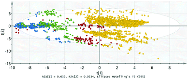
The SIMCA software utilises a few different methods to find correlations among the observations; note that it can also handle missing data. The first and simplest method is PCA (principal component analysis) which is typically used in conjunction with observations having only one type of variables (only X). Each observation, i.e. sample, is given a summary index number, made by summing variable values with given weights. SIMCA calculates each weight factor according to variable's importance in the model. When observations are plotted (score plot) according to their summary indexes, similar observations are located near each other, preferably forming groups. Also, a statistical confidence limit is calculated (Hotelling's T2; oval shape in plot), and observations lying outside this oval in the plot are potential outliers because of (i) bad/wrong data, or (ii) very different properties compared to the other observations. In Fig. 1, we present the PCA result for the present data based on the X variables, revealing clear group formation for example due to the choice of the A-site element. However, PCA is not able to tell why the groups are different in detail. From Fig. 1, very few (if any) true outliers can be distinguished indicating the high quality of the input data in general.
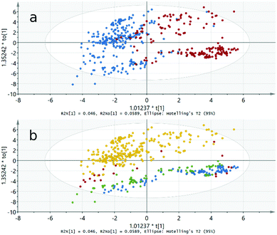
Next, we employ the so-called O2PLS (orthogonal partial least squares) model with DA (discriminant analysis) extension, which accepts multiple Y variables. This method is helpful in finding groups/subgroups among the sample set. In O2PLS score plots, horizontal variability indicates variance between the groups and vertical variability within the groups. This model works also with multiple observation classes, but for the simplicity we carry out the analysis for the following property-pairs separately: AFM-FM, AFM-PM and FM-PM.
Here we demonstrate the results of O2PLS-DA for the AFM-FM analysis in more detail. From the score plot shown in Fig. 2a it can first of all be seen that the AFM and FM compounds are in clearly separate groups. This manifests the fact that the type of magnetic ordering can indeed be predicted for the A2B′B′′O6 compounds based on simple chemical and structural parameters (such as those listed in Table 1). Moreover, from the plot in Fig. 2b it is seen that both the AFM and the FM compounds form two subgroups based on the A-site metal constituent depending whether the A metal is from the s-block or from the p-, d- or f-blocks. An interesting observation is (even though not specifically indicated in Fig. 2) that the FM compounds with the highest TC values are mostly located in the upper subgroup.
Also in the AFM-PM and FM-PM models the AFM or FM and PM compounds are divided into subgroups based on the A-site constituent (not shown here); however, it should be noted that for the PM compounds the A metal is in practice always from the s-block.
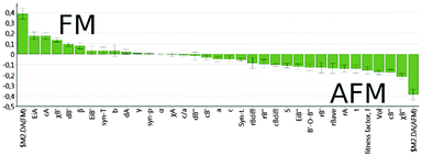
For all the models made, a so-called loadings plot can be constructed. This plot indicates the importance of the different variables in explaining the variability among the observations: the higher the weighting factor, the higher the importance of the variable. The O2PLS loadings plots also include auxiliary Y variables (located leftmost and rightmost in the loadings plot) indicating which variables affect each group/class the most. The same sign in both X and Y weighting factors indicates correlation and on the other hand, an opposite sign or a value close to zero indicates lack of correlation.
The loadings plot shown in Fig. 3 for our O2PLS-DA/AFM-FM model reveals that the most important variables defining an AFM compound are the B′′-site electronegativity and charge, and the unit cell volume, while for the FM compounds, the most influential variables are the ionization potential and charge of the A-site metal, and the electronegativity and electron configuration of the B′-site metal.
 | ||
| Fig. 3 O2PLS-DA/AFM-FM model loadings plot. Positive (on the left) weights are the most influential variables for the FM compounds and negative (on the right) for the AFM compounds. | ||
From a similar O2PLS-DA model for the FM-PM pair (not shown here) it may be concluded that the FM and PM compound groups start to show subgrouping when the B-site d-electron configuration is considered. In PM compounds, the B-site metals are of d0, d10 or fn configuration. On the other hand, in FM compounds the B-site cations are (in line with Goodenough–Kanamori–Anderson rules) either d3–d7 or d3–d8 type when the TC value is below room temperature. Compounds with TC above the ambient have usually d1/2/3/4/5–d3/4/5 combinations. It should also be noted that a tolerance parameter close to or above unity is preferred with compounds having high TC. The most influential parameters for FM compounds are the B-site electronegativity, cations coming from the d-block and the d-electron configuration.
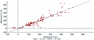
Finally, we test the predictive power of our FM model. For building the FM model we use a so-called training set, i.e. a dataset based on observations for which the ferromagnetism is confirmed and the TC value is known. In Fig. 4, we plot the experimentally observed TC values against the values predicted by our model for the same known FM samples. It can be seen that our model can predict the magnetic transition temperature with relatively good certainty for most of the samples. We then use the model to obtain TC values for a series of selected samples, whose chemical and structural properties have been described in literature, but whose magnetic properties are not known or reliably determined.
Among the selected “magnetically-unknown” samples there are naturally an extensive number of entries that are simply samples with stoichiometries and structural parameters very similar to those of the already known FM compounds, but which have not been characterized in their respective reference papers for their magnetic properties. These predictions rather serve as a model validation; the predicted TC values for these entries are indeed found to be nearly perfectly in line with the expectations. Most interestingly, we can also use the model to predict totally new promising FM material candidates. In particular, we can identify several unique candidate compositions for new FM double-perovskite compounds. For example, for La2CoFeO6,23 Pb2FeMoO6,24 Sr2CrRuO625 and La2CrFeO626 the magnetic properties are not known, but our model predicts TC values between 100 and 200 K. In Table 2 we summarize the predicted TC values for these promising A2B′B′′O6 FM candidate compounds.
Finally, we may utilize our FM model for qualitative prediction by looking at the most interesting FM compound families (with the highest TC values), like the A2CrReO6 compounds with A = Ca and Sr,27 and then search for the missing members in these families. In this respect, we note that Ba2CrReO628 and Ba2CoIrO629 exist in the hexagonal form but their perovskite forms have not been reported so far. Here it is important to emphasize that through high-pressure (HP) synthesis/treatment the required hexagonal-to-perovskite structure transformation could possibly be achieved, as there are a number of similar successful cases found in literature, such as Ba2FeSbO6,30 Ba2CoSbO6 and Ba2ZnTeO6.31
In conclusion, we have shown that with the present data, multivariate data analysis can distinguish A2B′B′′O6 double perovskite compounds based on their type of magnetism; their magnetic properties correlate with their chemical and structural properties, enabling us to predict the type of magnetic ordering and ordering temperature for new compounds. Such predictive power can greatly help in guiding further experiments for finding novel functional materials.
While this method can handle missing or poor data, it is still dependent on having good data for majority of the compounds in the training set. This suggests that our predictions could be greatly improved with additional measurements for already known compounds. For example, magnetic properties can be very sensitive to bond distances and angles. Thus, better structural data could improve the predictions of magnetic properties. Similarly, additional data on other physical properties, such as electrical, ionic or thermal conductivity, Seebeck coefficient, electrical polarization, or redox properties could help discovering new thermoelectrics, dielectrics, and battery and fuel-cell materials.
All of the compounds considered in this study were in bulk form. However, for technologically important applications, thin films are often required. Different substrates can cause strain/stress in the film, which can greatly affect the materials properties, as for example the magnetization in thin films of La2NiMnO6.32 Lattice mismatch, strain/stress and other such parameters could easily be added to our model, adapting it to new purposes as needed.
Conflicts of interest
There are no conflicts to declare.References
- S. Vasala and M. Karppinen, Prog. Solid State Chem., 2015, 43, 1 CrossRef CAS.
- P. Woodward, R.-D. Hoffmann and A. W. Sleight, J. Mater. Res., 1994, 9, 2118 CrossRef CAS.
- F. K. Pattersson, C. W. Moeller and R. Ward, Inorg. Chem., 1963, 2, 196 CrossRef.
- F. S. Galasso, F. C. Douglas and R. J. Kasper, J. Chem. Phys., 1966, 44, 1672 CrossRef CAS.
- T. Nakagawa, J. Phys. Soc. Jpn., 1968, 24, 806 CrossRef CAS.
- K.-I. Kobayashi, T. Kimura, H. Sawada, K. Terakura and Y. Tokura, Nature, 1998, 395, 677 CrossRef CAS.
- K.-I. Kobayashi, T. Kimura, Y. Tomioka, H. Sawada, K. Terakura and Y. Tokura, Phys. Rev. B: Condens. Matter Mater. Phys., 1999, 59, 11159 CrossRef CAS.
- J. Lindén, T. Yamamoto, M. Karppinen, H. Yamauchi and T. Pietari, Appl. Phys. Lett., 2000, 76, 2925 CrossRef.
- Y. H. Huang, R. I. Dass, Z. L. Xing and J. B. Goodenough, Science, 2006, 312, 254 CrossRef CAS PubMed.
- Y. H. Huang, R. I. Dass, J. C. Denyszyn and J. B. Goodenough, J. Electrochem. Soc., 2006, 153, A1266 CrossRef CAS.
- Y. H. Huang, G. Liang, M. Croft, M. Lehtimäki, M. Karppinen and J. B. Goodenough, Chem. Mater., 2009, 21, 2319 CrossRef CAS.
- F. D. Romero, S. J. Burr, J. E. McGrady, D. Gianolio, G. Cibin and M. A. Hayward, J. Am. Chem. Soc., 2013, 135, 1838 CrossRef PubMed.
- S. Vasala, J.-G. Cheng, H. Yamauchi, J. B. Goodenough and M. Karppinen, Chem. Mater., 2012, 24, 2764 CrossRef CAS.
- S. Vasala, H. Saadaoui, E. Morenzoni, O. Chmaissem, T.-S. Chan, J.-M. Chen, Y.-Y. Hsu, H. Yamauchi and M. Karppinen, Phys. Rev. B: Condens. Matter Mater. Phys., 2014, 89, 134419 CrossRef.
- S. Vasala, M. Avdeev, S. Danilkin, O. Chmaissem and M. Karppinen, J. Phys.: Condens. Matter, 2014, 26, 496001 CrossRef CAS PubMed.
- O. Mustonen, S. Vasala, E. Sadrollahi, K. P. Schmidt, C. Baines, H. C. Walker, I. Terasaki, F. J. Litterst, E. Baggio-Saitovitch and M. Karppinen, Nat. Commun., 2018, 9, 1085 CrossRef CAS PubMed.
- H. Yamauchi and M. Karppinen, Supercond. Sci. Technol., 2000, 13, R33 CrossRef CAS.
- Y. Syono, S.-I. Akimoto and K. Kohn, J. Phys. Soc. Jpn., 1969, 26, 993 CrossRef CAS.
- D. Iwanaga, Y. Inaguma and M. Itoh, J. Solid State Chem., 1999, 147, 291 CrossRef CAS.
- S. Vasala, H. Yamauchi and M. Karppinen, J. Solid State Chem., 2014, 220, 28 CrossRef CAS.
- K. Lehmus and M. Karppinen, J. Solid State Chem., 2001, 162, 1 CrossRef CAS.
- N. Imamura, T. Mizoguchi, H. Yamauchi and M. Karppinen, J. Solid State Chem., 2008, 181, 1195 CrossRef CAS.
- D. V. Karpinsky, I. O. Troyanchuk, K. Bärner, H. Szymczak and M. Tovar, J. Phys.: Condens. Matter, 2005, 17, 7219 CrossRef CAS.
- I. O. Troyanchuk, L. S. Lobanovsky, H. Szymczak and K. Bärner, J. Magn. Magn. Mater., 2000, 219, 163 CrossRef CAS.
- A. J. Williams, A. Gillies, J. P. Attfield, G. Heymann, H. Huppertz, M. J. Martínez-Lope and J. A. Alonso, Phys. Rev. B: Condens. Matter Mater. Phys., 2006, 73, 104409 CrossRef.
- A. K. Azad, A. Mellergård, S.-G. Eriksson, S. A. Ivanov, S. M. Yunus, F. Lindberg, G. Svensson and R. Mathieu, Mater. Res. Bull., 2005, 40, 1633 CrossRef CAS.
- H. Kato, T. Okuda, Y. Okimoto, Y. Tomioka, Y. Takenoya, A. Ohkubo, M. Kawasaki and Y. Tokura, Appl. Phys. Lett., 2002, 81, 328 CrossRef CAS.
- A. W. Sleight, J. Longo and R. Ward, Inorg. Chem., 1962, 1, 245 CrossRef CAS.
- J. F. Vente and P. D. Battle, J. Solid State Chem., 2000, 152, 361 CrossRef CAS.
- T. Tiittanen and M. Karppinen, J. Solid State Chem., 2017, 246, 245 CrossRef CAS.
- T. Aoba, T. Tiittanen, H. Suematsu and M. Karppinen, J. Solid State Chem., 2016, 233, 492 CrossRef CAS.
- H. Guo, J. Burges, S. Street, A. Gupta, T. G. Calvarese and M. A. Subramanian, Appl. Phys. Lett., 2006, 89, 022509 CrossRef.
Footnote |
| † Electronic supplementary information (ESI) available. See DOI: 10.1039/c8cc09579e |
| This journal is © The Royal Society of Chemistry 2019 |


