DOI:
10.1039/C9RA02150G
(Paper)
RSC Adv., 2019,
9, 18678-18687
Yield stress fluids and fundamental particle statistics
Received
20th March 2019
, Accepted 17th May 2019
First published on 14th June 2019
Abstract
Yield stress in complex fluids is described by resorting to fundamental statistical mechanics for clusters with different particle occupancy numbers. Probability distribution functions are determined for canonical ensembles of volumes displaced at the incipient motion in three representative states (single, double, and multiple occupancies). The statistical average points out an effective solid fraction by which the yield stress behavior is satisfactorily described in a number of aqueous (Si3N4, Ca3(PO4)2, ZrO2, and TiO2) and non-aqueous (Al2O3/decalin and MWCNT/PC) disperse systems. Interestingly, the only two model coefficients (maximum packing fraction and stiffness parameter) turn out to be correlated with the relevant suspension quantities. The latter relates linearly with (Young’s and bulk) mechanical moduli, whereas the former, once represented versus the Hamaker constant of two particles in a medium, returns a good linear extrapolation of the packing fraction for the simple cubic cell, here recovered within a relative error ≈ 1.3%.
Yield stress fluids form a particular state of matter,1 displaying non-linear and novel visco-plasto-elastic flow dynamics upon different boundary conditions. As their name says, they don’t flow until a certain load, the so-called yield stress (or point, τ0), is applied. This value may be generally interpreted as a shear stress threshold for the breakage of interparticle connectivity.2 Furthermore, as it initiates motion in the system, it is connected to mechanical inertia3 and particle settling, i.e. it is a terse summary of buoyancy, dynamic pressure, weight, viscous and yield stress resistances.4 For prototype systems such as colloids dispersed in a liquid, yield points sensibly depend on the mechanism by which the solid phase tends to interact or aggregate.5–8 The macroscopic constitutive equations they obey, such as the Herschel–Bulkley model, were shown to correspond, over a four-decade range of shear rates, to the local rheological response.9
From the side of an experimenter, however, unambiguously defining a yield stress may not always be straightforward. It can be affected by the experimental procedure adopted, always considering a measurement or some extrapolation technique with the limit of zero shear. Conversely, unyielded domains may be defined by areas where the shear stress second invariant falls below the yield value, plus some small semi-heuristic constant.10 In addition, theoretically, the meaning of notions like τ0 and rheological yielding were questioned to be only qualitative or even to stand for an apparent quantity.11 The dependence they generally show on timescales characteristic of the applied (mechanical) disturbance, also suggested an intimate relationship12 between yield stress and dispersion thixotropy.13 On the other hand, assigning a hydrodynamic or mechanical state below the yield point to a material that is not flowing seems not to be scientifically sound. Experimental values are normally obtained by extrapolation of limited data, whereas careful measurements below the yield point would actually imply that flow takes place.14
At any rate, the analysis of properly defined τ0 concepts forms the subject of interesting investigations and is still a powerful tool in many applications, including macromolecular suspensions,15 gels, colloidal gels and organogels,16–18 foams, emulsions and soft glassy materials.19 It allows for effective comparisons between the resistances which fluids initially oppose to the shear perturbation, somehow specifying a measure of the particle aggregation states taking place in a given dispersant. Electrorheological materials, for instance, exhibit a transition from liquid-like to solid-like behaviors, which is often examined by a yield stress investigation upon a given fluid model (e.g. the Bingham model or the Casson model).20,21 The combination of yield stress measurements with AFM techniques can be used to well-characterize the nature of weak particle attractions and surface forces at nN scales.8 Further issues of a more geometrical nature, which naturally connect to τ0, are rheological percolation22 and its differences from other connectivity phenomena, such as the onset of electric23 or elastic percolation.24,25 In granular fluids, it relates with the theory of jammed states,26 originally pioneered by Edwards.27
In nanoscience as well, the stability control and characterization in single and mixed dispersions or melts is an important and complex step.28,29 Carbon nanotube suspensions,30 for example, can be prepared in association with other molecular systems, like surfactants and polymers31–33 or by (either covalent or non-covalent) functionalization of their walls with reactive groups, which increases the chemical affinity with dispersing agents.34 As a consequence of large molecular aspect ratios and significant van der Waals’s attractions, the nanotube aggregation is highly enhanced, giving rise to strongly anisotropic systems of crystalline ropes and entangled network bundles, which are difficult to exfoliate, suspend or even characterize.35 Stable CNT dispersions of controlled molecular mass may also exhibit polymeric behavior, and be quantitatively studied by equations taken from the well-established science of macromolecules.36,37
This paper puts forward a basic approach, mostly focused on equilibrium arguments, to devise a yield stress law connected with particle statistics. By conjecturing an ensemble of effective volumes ‘displaced’ at the incipient state of motion, a statistical mechanics picture of τ0 is proposed. This affords a phenomenological hypothesis that can be developed with reasonable simplicity. The derived relations are applied to typical disperse systems in colloid science and soft matter, such as aqueous and nonaqueous suspensions of ceramic/metal oxides and nanoparticles.
Defining an ensemble of volumes at the incipient motion
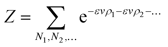
Yield stresses can be generally written as a sum of pairwise bonding contributions, where each particle pair is assigned a larger volume than the juxtaposition of the two initial units,38,39 or by averaging the geometric part of the Hamaker expression over a representative pairwise cell.6 This analysis relies instead on a statistical definition of an effective volume concept (Vd) in a thought experiment. We suppose that, in yielding a dispersion, a canonical ensemble of volumes is displaced from the rest configuration and fulfils well defined statistical laws in thermal equilibrium, at a constant particle number and dispersion volume. The energy perturbation at the onset of motion will diminish with an increasing solid fraction in a representative large cell Vd, reflecting an increase in τ0.
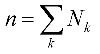
The disperse system will be conjectured to consist of an ensemble of elementary cells, each containing or not containing at least an aggregated solid unit (onwardly referred to as the “cluster” = cell + aggregates). An equilibrium total cluster number then can be identified with a conserved sum of aleatory variables (Nk):
| |
 | (1) |
whose values specify the aggregation statistics in each cell
k. In the simplest limit cases, one may assign (A) a two-valued set,
Ni = {0,1}, meaning that the
i-th cell will be respectively empty or occupied by an aggregate, or (B) it may take any integer value,
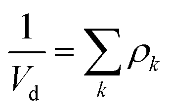
Ni = {0,1, … ∞}, defining in the extreme case, a cell that would be capable of hosting an open aggregate number. We complete this definition by a second relationship for the portions of fluid displaced in the experiment, conceived for simplicity as a set of discrete terms obeying the following combination law of volumes:
| |
 | (2) |
where
ρk =
Nk/
Vk is the
k-th cluster density, and
Vk is the
k-th contribution to
Vd. Yield strength will reflect the configuration statistics over the ensemble. Any cell containing aggregates will contribute to it, otherwise it won’t affect
τ0 (see
Fig. 1). In ‘simple’ yield stress fluids, rest interactions are known to prevent the aggregation structure from breaking as a consequence of thermal agitation, and slow flows display a plastic behavior at very large deformations, without irreversible structural variations.
1,40 However, the equation systems
(1) and
(2) will be supposed to generally hold and be adopted irrespective of specific fluid dynamics properties (
e.g. thixotropy or shear-thinning, pseudo-plasticity,
etc.). Note that the density concept which the first two equations refer to does not coincide with the average dispersion density. The aim is to define an
ad hoc (
i.e. apparent, quasi-static) solid fraction value by which the yield stress response can be obtained by a statistical mechanics approach at the incipient state of motion.
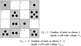 |
| | Fig. 1 Scheme of the fluid cluster structure at the incipient motion. Cell volumes aren’t necessarily equal, as depicted here. Those in grey, with cell occupancy larger than zero, contribute to eqn (2). | |
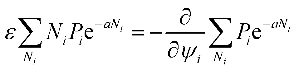
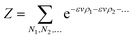
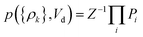
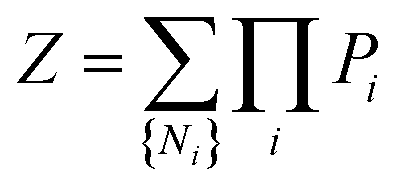
A criterion assigning a sum over aggregation states is required for a thermodynamic framework, with this being promptly done by the usual partition function concept:
| |
 | (3) |
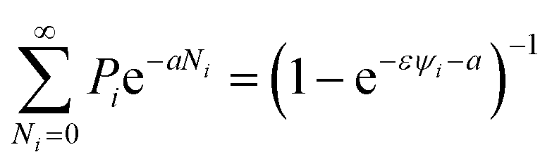
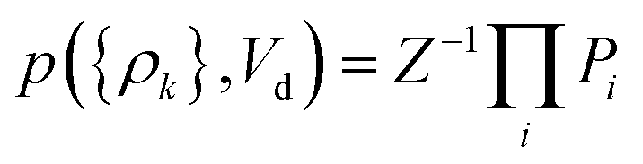
To give a suitable representation of the statistical issue, we define Pi = Pi(v,Vi) to be the probability of finding in Vi an empty (liquid) portion of volume v or, equivalently, an empty volume fraction ψi ≡ v/Vi. As we will tackle enough concentrated systems, this choice is suitable for an application of Poisson’s statistics. For spherically symmetric units and negligible excluded volumes, an expression like:
may be adopted,
41 implying:
| |
 | (5) |
with normalized canonical probabilities, constrained to
eqn (1) and
(2):
| |
 | (6) |
The quantity ε is introduced as a measure of cluster–cluster interaction strength,42 and regarded for simplicity as a homogeneous stiffness parameter, independent of {ρi}. The volume fraction ψi is a characteristic of the implied aggregation state.
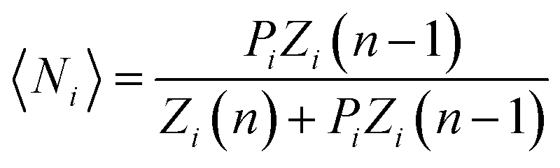
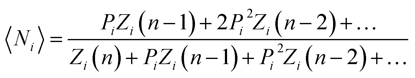
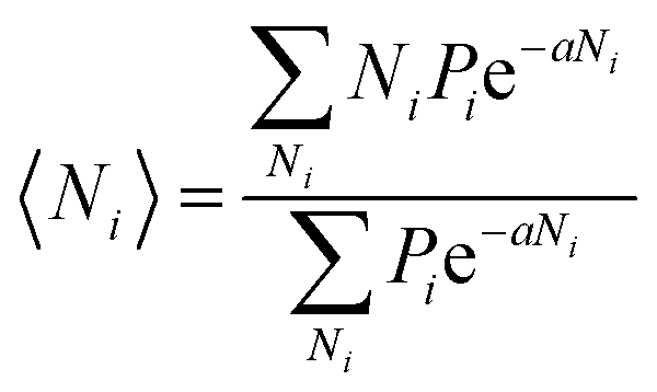
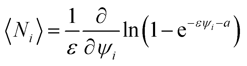
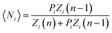
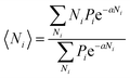
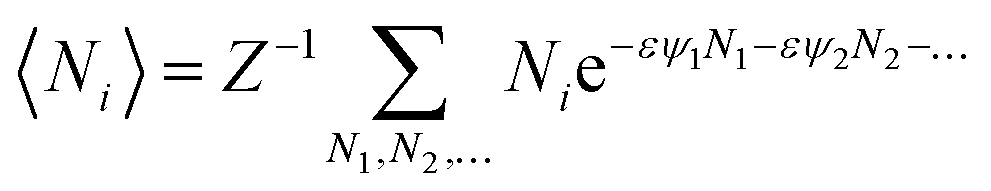
We will relate the average occupancy in a generic single-particle state to the cluster interaction extent, and thus to τ0. Particle indistinguishability, which is commonly a non-classical feature (but not only, see e.g. ref. 43), will be retained in this framework. From the rules of statistical mechanics, one therefore gets:
| |
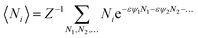 | (7) |
that, in light of
eqn (2), may be rewritten as:
| |
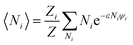 | (8) |
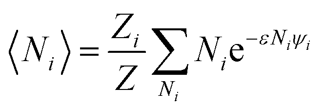
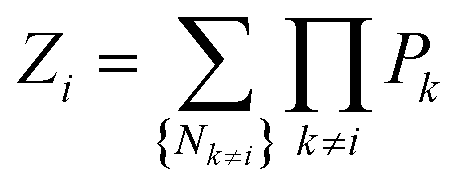
Here,
Zi denotes the partition function with state
i omitted:
| |
 | (9) |
i.e. corresponding to the restricted sum:
| |
 | (10) |
Developing eqn (8) returns a distribution of (A) Fermi–Dirac or (B) Bose–Einstein type, and the proof of such a formal analogy is resumed in Appendix 1 upon mapping:
with
kBT being the Boltzmann thermal energy. This phenomenological equation redefines an effective volume fraction in the displaced fluid (
Fig. 2). It has an intuitive significance, as energy perturbations (
Ek) will increase with increasing temperature, stiffness parameter and the velocity perturbation at the onset of motion, reflected by a larger liquid fraction (
ψk),
i.e. conditions normally implying a smaller yield stress. In the next section, some observations on fractional statistics, lying between (A) and (B), are reported as well the introduction of an intermediate state (C).
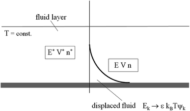 |
| | Fig. 2 Sketch of the canonical volume ensemble. Total volume V + V*, energy E + E*, and individual particle numbers are held constant, with n ≪ n*. | |
Finally, an equivalence between volume and energy was formerly introduced by Edwards and Oakeshott, although in a different context.27 Their pioneering theory of powders faced the issue of a statistical mechanics analysis of non-thermal systems, like granular fluids.
Yield stress and cluster statistics
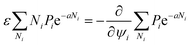
The most general pressure equation is written as a microscopic average of the stress tensor over the statistical distribution of particle states, provided here by eqn (7).44 As yield stresses are likewise expected to be linear combinations of 〈Ni〉 with unknown (tensor) coefficients, we specialize the calculation to the mean cluster occupancy in the overall representative state conjectured by eqn (2):| |
 | (12) |
i.e.:
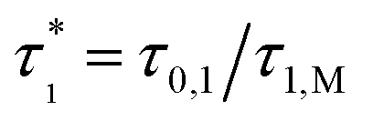
The proportionality constant in this relationship will be removed by forming the experimental quantity τ* = τ0/τM, i.e. dividing by the largest stress within a class of homogeneous and comparable measurements.
In (A), with a two-valued statistics, the arrangement of particle clusters takes the form (Appendix 1):
| | |
〈Ni〉 = (ea+εψi + 1)−1
| (14) |
with
a being a characteristic fluid property, expressible as:
for some aggregation state denoted by
ψa. It describes a liquid volume fraction at which the distribution function may either show a phase-like transition or a (rheological) percolation point.
23 Correspondingly,
ε gives a measure of the average rate at which
τ0 is changing near
ψa. The yield stress value as a function of
ψ thus reads:
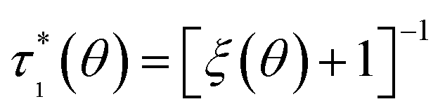
| | |
τ0,1(ψ) = [eε(ψ−ψa) + 1]−1
| (16) |
and, as the solid fraction
θ complementing
ψ obeys:
the normalized distributions of values in
θ will scale as:
| |
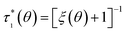 | (18) |
still with

, with
θa being a critical threshold/maximum packing density, and:
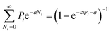
In (B), the expression for an infinitely-valued statistic is regained as:
| | |
〈Ni〉 = (ea+εψi − 1)−1
| (20) |
so that:
| |
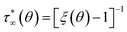 | (21) |
Note that, as this distribution approaches infinity for ξ → 1+, it can no longer be normalized to unity. The idealized situation in which cells are permitted to be indefinitely occupied corresponds to the steepest liquid–solid transitions or percolation points contemplated by the model in its present form.
When the maximum cell occupancy is neither unitary nor infinite, it can be proven that:45
| |
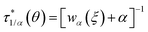 | (22) |
upon validity of the implicit relation
wαα(1 +
wα)
1−α =
ξ(
θ),
α ∈ [0,1] ∩
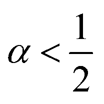
Q. This parameter,
α ≤ 1/〈
Nr〉, gives a terse summary of the fractional interaction state, the extreme limits of which return type A (
α = 1) and B (
α = 0) laws. In between, an intermediate ‘statistical interaction’ follows, being attractive or repulsive depending respectively on whether

or

.
46 A general treatment of α-states would raise tough formal and numerical issues, falling beyond the experimental verification purposes of this work. In the next section, we thus limit ourselves to the neutral state

(type C), which can be solved explicitly (
e.g. 
) to return
.
45 The semi-heuristic position
wα′(
ξ) ≡
ξ, now with
α′ ∈ [−1,1], would be rather convenient for an intuitive data analysis, but is formally inadequate for a model comparison, and is therefore disregarded.
Results and discussion
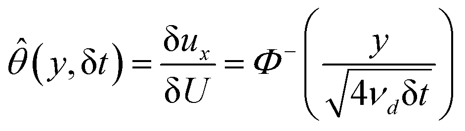
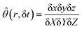
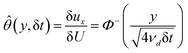
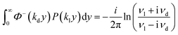
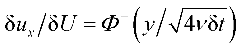
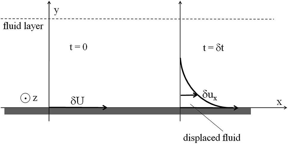
Yield stress measurements are normally reported against solid fractions like the volumetric (ϕ) or the mass concentration. To get the dependence ξ = ξ(ϕ), consider a fluid layer bounded on one side by the plane surface xz. For a flow perturbation implied by a constant velocity δUex exerted at the surface, the velocity component x at a distance y from the plane will obey the profile 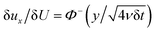 , in which ν is the kinematic viscosity and δt is a small time interval.47 The complementary error function, denoted by Φ−, quantifies the velocity fraction transmitted to the fluid upon shearing, and thus can be adopted for the evaluation of θ illustrated in Fig. 3 and explained in detail in Appendix 2.
 |
| | Fig. 3 Fluid dynamics scheme for evaluating θ. | |
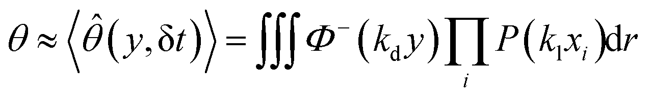
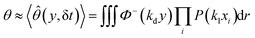
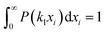
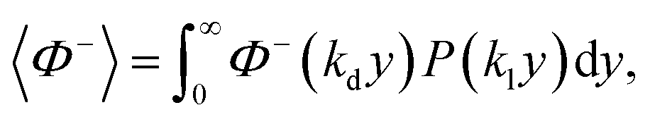
If the velocity profile is averaged over an incompressible liquid flow undergoing free momentum diffusion (no pressure gradient or volume forces, nor hydrodynamic perturbations, see the remarks in Appendix 2), the solid fraction can be estimated as:
i.e.:
| |
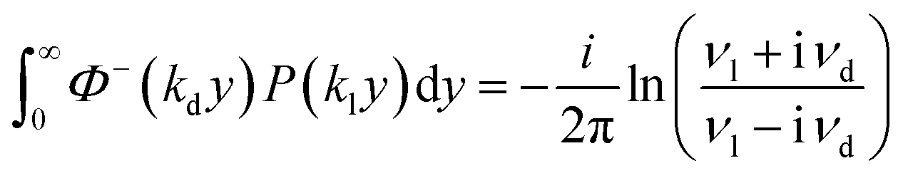
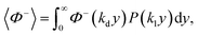 | (24) |
with
(
i =
d, dispersion;
l, liquid) and
P being a Gaussian function. This integral turns out to be well defined, as it is time-independent, and only depends upon
ϕ through the ratio
kd/
ki:
| |
 | (25) |
Here
![[small nu, Greek, macron]](https://www.rsc.org/images/entities/i_char_e0ce.gif)
≡
νd/
νl =
![[small eta, Greek, macron]](https://www.rsc.org/images/entities/i_char_e0c8.gif)
/
![[small rho, Greek, macron]](https://www.rsc.org/images/entities/i_char_e0d1.gif)
, with shear viscosity and mass density being expressible as
ηd =
ηl(
ϕ) and
ρd =
ρl(
ϕ),
i.e. the product of pure liquid properties times a function of the solid fraction. The reduced quantity
=
(
ϕ) generally increases with increasing
ϕ, since viscosity changes should dominate over
ρ values in the concentration regimes of interest. Correspondingly, a larger fluid inertia leads to a reduction of
ψ (
eqn (16)), as expected. Note that a critical threshold/maximum packing density (
ϕa) cannot be identified from the last equation, being

. A boundary/cutoff value
θa ≡
ϕa needs to be set independently, completing the definition of
ξ =
ξ(
θ) in the previous relationships, with the requirement
θ <
ϕa, or:
| | |
(ϕ) < tan(πϕa)
| (26) |
representing a model constraint for the viscosity, density and the critical volume fraction. Applications of the new equation family will be conducted in conformity with it, as shown in
Fig. 7. While
eqn (26) always depends on the viscosity model, it is more selective for B and C statistics (
α < 1), describing steeper liquid–solid transitions.
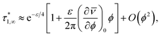
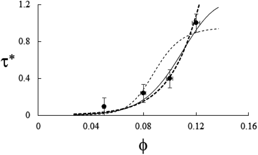
Eqn (25) redefines an effective volume fraction, ϕ → θ(ϕ). To test its validity, experimental measurements from aqueous and non-aqueous systems were taken from the literature. In the first case, the yield stress of ceramic and metal oxide dispersions of Si3N4,5,6 α-Ca3(PO4)2,5,6 ZrO2,48 and TiO2 (ref. 49) (anatase) were regarded, whereas Al2O3/decalin50 and multiwalled carbon nanotubes/polycarbonate51 (MWCNT/PC melts) were regarded as non-aqueous materials. In these systems, interaction mechanisms were mostly London–van der Waals with absent or irrelevant Vold’s effect.52 The first three were at/near their isoelectric points, where double-layer surface charges are negligible.53 The structure of the anatase colloids was governed too by attractive van der Waals forces, which represents the main interaction mechanism in the last system as well.54 Compressive yield stress in the fifth system, alumina in decalin, was still of the van der Waals type, modulated by a steric interparticle repulsive barrier of ∼0.7 nm of propionic acid, with no further electrostatic or structural energies coming into play. With the obvious exception of MWCNT/PC melts (T ≃ 533 K), all measurements were conducted at room temperature. The adopted extrapolation laws were Casson or Bingham, unambiguously written in the yield stress, viscosity, and shear rate, with no heuristic constants. In Al2O3 systems, compressive yield stresses were numerically inferred from the measured variation of volume fraction solids with elevation. Any further physical chemistry details may be found in the references.
Every plot of  vs. ϕ was best fitted by means of each particle statistic, 1/α = 1 (A), ∞ (B), 2 (C) and the extracted model parameters are depicted in Table 1. Shear viscosity data vs. solid concentration were available for the system MWCNT/PC55 and fulfilled Eiler’s law,
  (e.g. ref. 56), where a large intrinsic viscosity value ([η] = 165) seems to be a feature of other carbon nanotube suspensions.57 Quemada’s model, (ϕ) = (1 − ϕ/ϕa)−2, was generally adopted in the other systems, still producing a good agreement with yield stress profiles. Examples of the suitability of each model is shown in Fig. 4–6, while Fig. 7 shows how the model constraint in eqn (26) is fulfilled in these cases. Obviously, a similar agreement is also found for Ca3(PO4)2/H2O, ZrO2/H2O, and Al2O3/C10H18.
Table 1 Yield stress model parameters
| Chemical system (s/ l) |
α |
ϕa |
ε |
| Si3N4/H2O |
 |
0.452 |
31.7 |
| Ca3(PO4)2/H2O |
0 |
0.509 |
10.5 |
| ZrO2/H2O |
 |
0.393 |
26.1 |
| TiO2/H2O |
0 |
0.523 |
18.6 |
| Al2O3/C10H18 |
0 |
0.527 |
30.9 |
C/(–O–(C![[double bond, length as m-dash]](https://www.rsc.org/images/entities/char_e001.gif) O)–O–)n O)–O–)n |
1 |
0.443 |
69.8 |
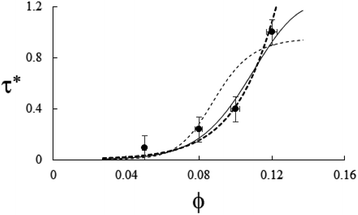 |
| | Fig. 4 Example of particle statistics α = 0. Reduced yield stress versus solid volume fraction for the anatase system TiO2/H2O (densely dashed line, α = 0; dashed line, α = 1; solid line,  ). Model parameters for α = 0 are in Table 1. Best fits with similar quality were also met in Ca3(PO4)2/H2O and Al2O3/C10H18 systems. ). Model parameters for α = 0 are in Table 1. Best fits with similar quality were also met in Ca3(PO4)2/H2O and Al2O3/C10H18 systems. | |
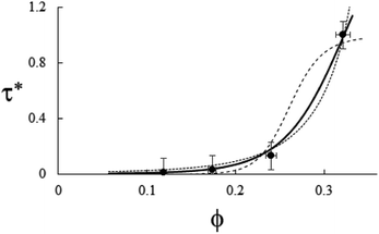 |
| | Fig. 5 Example of particle statistics  . Reduced yield stress versus solid volume fraction for Si3N4/H2O. Lines and symbols are as in Fig. (4), and model parameters for . Reduced yield stress versus solid volume fraction for Si3N4/H2O. Lines and symbols are as in Fig. (4), and model parameters for  are in Table 1. Best fits with similar quality were also obtained in ZrO2/H2O. are in Table 1. Best fits with similar quality were also obtained in ZrO2/H2O. | |
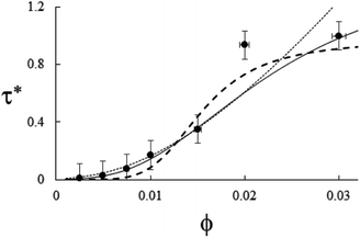 |
| | Fig. 6 Example of particle statistics α = 1. Reduced yield stress versus solid volume fraction for MWCNT/PC. Lines and symbols are as in Fig. 4, and model parameters for α = 1 are in Table 1. | |
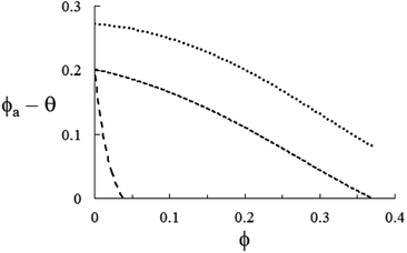 |
| | Fig. 7 Representation of eqn (26) in each of the instances in Fig. 4–6 with = 1 + (ρs/ρl − 1)ϕ. From the top, TiO2/H2O (ρs/ρl ≈ 4.23, short-dashed), Si3N4/H2O (ρs/ρl ≈ 3.17, medium-dashed) and MWCNT/PC (ρs/ρl ≈ 1.17, long-dashed). As expected, each of the functions θ–ϕa is always positive in the respective experimental domain, ϕ ≤ 0.12 (TiO2), ϕ ≤ 0.32 (Si3N4), and ϕ ≤ 3 × 10⁻² (MWCNT). | |
Single-valued distribution (A) is the only one predicting a plateau, as is the evident case here of MWCNT/PC melts. A similar situation arises from kaolin colloids in water, paraffinic oil and liquid polybutadiene rubber, for which an S-shaped functional form analogous to eqn (18) was proven to hold.58,59 Unluckily, the sparseness of physical chemistry properties of kaolin powders, especially when commercially supplied, do not allow for a data comparison with the other chemical systems, in Tables 1 and 2. Furthermore, the present model turns out to be fundamentally non-linear. Since chemical compositions of kaolin materials are markedly heterogeneous, to average over distinct solid components would require an extension of this approach to the framework of multi-phase media. Finally, on increasing α, (B) and (C) distributions imply steeper behaviors, as they are usually indicative of stronger interactions. Improving the agreement in Fig. 6 likely requires the combination of further interaction states.
The maximum solid loading is known exactly in two cases, the first of which, ϕm = 0.54 (Al2O3/C10H18),50 agrees with ϕa ≈ 0.53 in Table 1. Volume corrections due to propionic acid layers were estimated to be less than 1%. The second, ϕm = 0.146 (TiO2/H2O), was highly affected by porosity (nanoparticles forming an interlinked porous network in the liquid) and thus is not directly comparable with ϕa.49 The fraction ϕa was reported at the third digit, as the model was sensitive to it.
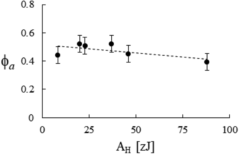
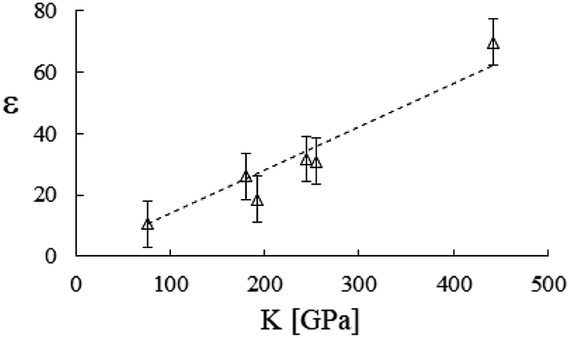
To interpret the model parameters by the extent of particle interactions, relevant energetic quantities at mesoscopic/macroscopic scales were collected in Table 2, i.e. the Hamaker constant for particles in the dispersant (AH), which reflects the difference between the polarizabilities of solid and liquid molecules, and Young’s/bulk moduli of the solid phase (E, K), defining the elastic response in homogeneous isotropic materials. While AH is known to relate with τ0,6,48 elastic (and loss) moduli, detected from oscillatory tests at ∼1 Hz, were recently found to be proportional to the yield stress of gel (Carbopol) solutions.9
Table 2 Particle–particle interactions and elastic solid constants
| Chemical system (s/l) |
AH [zJ] |
E [GPa] |
K [GPa] |
| Si3N4/H2O |
46 |
320 |
245 |
| Ca3(PO4)2/H2O |
23 |
104 |
76 |
| ZrO2/H2O |
88 |
241 |
181 |
| TiO2/H2O |
37 |
167 |
192 |
| Al2O3/C10H18 |
20 |
400 |
255 |
| C/(–O–(CO)–O–)n |
8 |
740 |
442 |
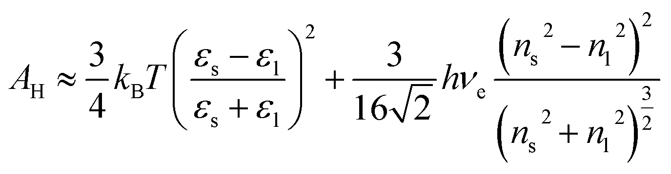
The aqueous Hamaker constant was determined by the knowledge of optical spectra of Si3N4 (ref. 60) and ZrO2 (ref. 61) from Lifshitz theory. For TiO2, it was deduced from linearly correlating yield stress data with the square zeta potential.62 As in the case of colloidal Al2O3 in decalin,50 the Tabor–Winterton approximation was adopted to evaluate AH of tricalcium phosphate particles. Upon neglecting retardation effects, it gives:63
| |
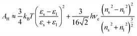 | (27) |
with refractive indices in the visible spectrum set to
ns ≈ 1.6, and
nl = 1.33 and static dielectric constants
εs ≈ 15.4, and
εl = 80. The UV absorption frequency should range here in (
ref. 63) (3–4) × 10
15 Hz so that a mean
ve ≈ 3.5 × 10
15 Hz was assumed. Because data for α-Ca
3(PO
4)
2 are scarce,
ns is inferred from optical spectra of calcium phosphate glasses
64 in the proportion [CaO]
![[thin space (1/6-em)]](https://www.rsc.org/images/entities/char_2009.gif)
:
[P
2O
5] = 1
:
3 and
εs is that of hydroxyapatite, as it was successfully employed in a DLVO theory for amorphous particles.
65 The Hamaker constant for MWCNT/PC was also evaluated, from the combining law
66 for the pure materials values
AsH ≈ 100 zJ (
ref. 67) and
AlH = 50.8 zJ:
68| |
 | (28) |
Elastic features were taken from rather recent literature on each of the solid compounds listed in the tables. For Si3N4, an average E value among three families of samples was considered, which is then representative of Ceradyne Ceralloy.69 Near-theoretical density values were adopted for Al2O3 (ref. 69) and K of β-Si3N4,69 which was the most abundant silicon nitride phase (∼84.4% wt) in the original fluid samples of Fig. 5.70 The Young’s modulus for α-Ca3(PO4)2 was experimentally measured, with the bulk one being calculated instead using ab initio density functional theory calculations (DFT),71 i.e. the same numerical framework employed to get the elastic constants of TiO2 (anatase)72 and ZrO2.73 Average values between the predictions from generalized gradient (GGA) and local density approximations (LDA) were regarded for the monoclinic ZrO2 phase. Concerning MWCNT, E was taken from an atomistic potential simulation,74 whereas the diamond value was used for K.75
To proceed, the quantitative insight now is to link AH to ϕa, and E, K to ε. On increasing the extent of the repulsive forces, particles exhibit an effective size (re) and volume fraction (ϕe), relating with unperturbed values as76 ϕ/ϕ* = (r/r*)3.
Accordingly, by representing ϕa = ϕa(AH), one can verify a meaningful linear correlation that extrapolates, in the limit AH → 0+, a good estimate for the packing fraction of the simple cubic cell, ϕa (0+) = 0.517 against π/6 ≈ 0.524 (Fig. 8). Regarding ε = ε(E, K), it still shows a reasonable linear trend with both elastic constants (Fig. 9 and 10). As expected upon E, K → 0+, the stiffness parameter ε(0+) → 0 as well. The behaviors in Fig. 8–10 did not vary appreciably upon changing the yield stress data from Bingham to Casson, which were both available for anatase.49
 |
| | Fig. 8 Packing fraction versus the Hamaker constant, best fitted by ϕa = 10−3 × (517.2 − 1.2AH). Data from Table 2. | |
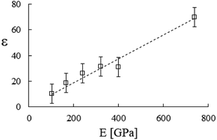 |
| | Fig. 9 Stiffness parameter versus the Young’s modulus, best fitted by ε = 9.3 × 10⁻²E [GPa]. Data from Table 2. | |
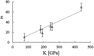 |
| | Fig. 10 Stiffness parameter versus the bulk modulus, best fitted by ε = 14.0 × 10⁻²K [GPa]. Data from Table 2. | |
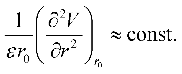
Such correlations, especially with the Young’s modulus, are suggestive of a linear law between ε and the interatomic spring constant of the solid compounds, consistent with a microscopic definition of the stiffness parameter, i.e.:
| |
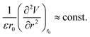 | (29) |
where
V =
V(
r) is the bond energy and its curvature is calculated at the equilibrium interatomic distance
r =
r0. The constant term on the right identifies an intrinsic elastic modulus, as it would promptly follow from the knowledge of potential energy details (
e.g. Lennard-Jones) combined with the best fit of
ε vs. E.
In conclusion, it is noteworthy to point out a couple of formal issues met in this analysis. First, the equations for τ0 cannot be reduced to a power law in ϕ where, as in fractal-like structures, the exponent is expected to account for the interaction rate.76 This doesn’t mean, evidently, that (B) or (C) distributions would not yield good numerical approximations for such cases as well. Second, the model inadequacy to reproduce  in the limit of infinite dilution is anyway recovered upon ε → ∞. The actual values of stiffness parameters should guarantee a rather fast convergence since, for (A) and (B) distributions with
  and
and  :
:
| |
 | (30) |
the numbers in Table 1 reasonably return  when ϕ → 0+.
Conclusive remarks
Solid concentration affects the properties of complex fluids, and we put forward the (re)definition of an effective volume fraction (θ) for the yield stress behavior, here evaluated in terms of a reduced kinematic viscosity. Aggregation clusters contributing to τ0 are modelled by canonical ensembles of (displaced) volumes, with particle statistics determined by the occupancy number.
This conjecture points out an average cluster that is representative of the incipient state of motion, with given liquid and solid fractions. A class of statistical mechanics laws defines yield stress in terms of two coefficients, the maximum packing threshold (ϕa) and the particle stiffness parameter (ε), e.g.:
| | |
1/τ0(ϕ) ∼ e−ε[θ(ϕ)−ϕa] ± 1
| (31) |
which turn out to relate to the Hamaker constant and elastic moduli of the solid phase.
Conflicts of interest
There are no conflicts to declare.
Appendixes
Appendix 1
We resume here some of the well known results for eqn (8) in (A) and (B).77 In comparison to the original theories, the energy of the level k(Ek) is mapped initially into ψk, the Boltzmann energy (kBT) into 1/ε and the chemical potential (μ) into ψa. In fact, the energy representation is regained upon eqn (11).
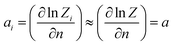
Consider thus the restricted partition function specified by eqn (9) and (10). In (A), the mean particle number in a state i reads:
| |
 | (A.1) |
where, to work it out, the following expansion can be used upon Δ
n/
n ≪ 1:
| | |
lnZi(n − Δn) ≈ lnZi(n) − aiΔn
| (A.2) |
and, for a sum over many states, the following approximation:
| |
 | (A.3) |
implies:
| |
 | (A.4) |
Replacing this result into eqn (A.1) proves eqn (14). In (B), let’s use the former logarithmic expansion:
| |
 | (A.5) |
to get:
| |
 | (A.6) |
the numerator of which is expressible through:
| |
 | (A.7) |
Obviously, after noting the infinite geometric series:
| |
 | (A.8) |
Eqn (20) is recovered at once, since:
| |
 | (A.9) |
Remember that eqn (A.3) upon eqn (11) gives a = −μ/(kBT). We accordingly interpret the ratio −a/ε in the corresponding relationship to assign a characteristic aggregation state of the disperse system (a percolation-like point ψa) in every statistic here regarded.
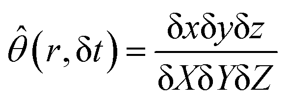
Appendix 2
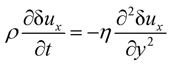
For the incompressible flow in Fig. 3, with δuy = δuz = 0, with no pressure gradient and volume forces, the balanced equation for the momentum along x brings us to:| |
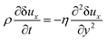 | (B.1) |
where the constants, ρ and η, denote the mass density and shear viscosity coefficient. This is the basic equation to get the complementary error function and the Gaussian probability distribution in eqn (24).
To evaluate the fraction θ in eqn (17), we form the quantity:
| |
 | (B.2) |
with each displacement at the numerator being time-dependent, with δ
Xi = δ
xi (0). Since no perturbation develops along
y and
z, one has δ
y/δ
Y = δ
z/δ
Z = 1, and:
| |
 | (B.3) |
where δ
x/δ
ux = δ
X/δ
U = δ
t. To average the solid fraction and eliminate the dependencies on time and space, we limit ourselves to the free momentum distribution (
P) in the liquid flow and disregard perturbations from long-ranged hydrodynamic interactions among particles.
78 They are expected to be negligible upon decreasing speed at the incipient motion
79 and increasing dilution of the dispersed units.
80 Hydrodynamic back-flows may be effectively screened as well by charged particles,
81 while in systems like complex fluid interfaces they are generally not.
82
Therefore, still with the same notations of eqn (24), it turns out that (xi = x,y,z):
| |
 | (B.4) |
which, since:
| |
 | (B.5) |
and:
| |
 | (B.6) |
reduces, after some mathematical developments, to
eqn (25).
Acknowledgements
Jordi Sancho-Parramon and Prabhu Nott are acknowledged for their useful remarks. This work started years ago and was partly supported by a former Italian MURST (40%).
References
- P. Coussot, Rheol. Acta, 2017, 56, 163–176 CrossRef CAS.
- P. Coussot, Rheol. Acta, 2018, 57, 1–14 CrossRef CAS.
- R. R. Huilgol, Phys. Fluids, 2002, 14, 1269–1283 CrossRef CAS.
- A. Wachs and I. A. Frigaard, J. Non-Newtonian Fluid Mech., 2016, 238, 189–204 CrossRef CAS.
- S. A. Mezzasalma, J. Colloid Interface Sci., 1997, 190, 302–306 CrossRef CAS.
- S. A. Mezzasalma, Phys. Rev. E: Stat. Phys., Plasmas, Fluids, Relat. Interdiscip. Top., 1998, 57, 3134–3141 CrossRef CAS.
- G. V. Franks, J. Colloid Interface Sci., 2002, 249, 44–51 CrossRef CAS PubMed.
- E.-J. Teh, Y.-K. Leong, Y. Liu, V. S. J. Craig, R. B. Walsh and S. C. Howard, Langmuir, 2010, 26, 3067–3076 CrossRef CAS PubMed.
- J. Boujlel and P. Coussot, Soft Matter, 2013, 9, 5898–5908 RSC.
- A. R. Koblitz, S. Lovett and N. Nikiforakis, Physical Review Fluids, 2018, 3, 023301 CrossRef.
- H. A. Barnes, J. Non-Newtonian Fluid Mech., 1999, 81, 133–178 CrossRef CAS.
- P. Coussot, Q. D. Nguyen, H. T. Huynh and D. Bonn, Phys. Rev. Lett., 2002, 88, 175501 CrossRef PubMed.
- M. Jenny, S. Kiesgen de Richter, N. Louvet, S. Skali-Lami and Y. Dossmann, Physical Review Fluids, 2017, 2, 023302 CrossRef.
- B. Coleman, H. Markovitz and W. Noll, Viscometric Flows of Non-Newtonian Fluids: Theory and Experiment, Springer, Berlin, 1966 Search PubMed.
- P. Samyn and H. Taheri, J. Mater. Sci., 2016, 51, 9830–9848 CrossRef CAS.
- F. Yang, K. Paso, J. Norrman, C. Li, H. Oschmann and J. Sjöblom, Energy Fuels, 2015, 29, 1368–1374 CrossRef CAS.
- C. Zhao, G. Yuan, D. Jia and C. C. Han, Soft Matter, 2012, 8, 7036–7043 RSC.
- A. Chakrabarty and U. Maitra, J. Phys. Chem. B, 2013, 117, 8039–8046 CrossRef CAS PubMed.
- G. Ovarlez, Q. Barral and P. Coussot, Nat. Mater., 2010, 9, 115 CrossRef CAS PubMed.
- H. J. Choi and M. S. Jhon, Soft Matter, 2009, 5, 1562–1567 RSC.
- S. A. Mezzasalma and G. J. Koper, Colloid Polym. Sci., 2002, 280, 160–166 CrossRef CAS.
- A. K. Kota, B. H. Cipriano, M. K. Duesterberg, A. L. Gershon, D. Powell, S. R. Raghavan and H. A. Bruck, Macromolecules, 2007, 40, 7400–7406 CrossRef CAS.
- D. Stauffer and A. Aharony, Introduction to Percolation Theory, 1985 Search PubMed.
- S. Arbabi and M. Sahimi, Phys. Rev. Lett., 1990, 65, 725–728 CrossRef CAS PubMed.
- M. Sahini and M. Sahimi, Applications Of Percolation Theory, CRC Press, London, 1994 Search PubMed.
- P. Ball, Nat. Mater., 2016, 15, 1227 CrossRef CAS PubMed.
- S. Edwards and R. Oakeshott, Phys. A, 1989, 157, 1080–1090 CrossRef.
- C. Zhao, G. Yuan, D. Jia and C. C. Han, Soft Matter, 2012, 8, 7036–7043 RSC.
- M. T. Zafarani-Moattar and R. Majdan-Cegincara, Fluid Phase Equilib., 2013, 354, 102–108 CrossRef CAS.
- E. K. Hobbie and D. J. Fry, J. Chem. Phys., 2007, 126, 124907 CrossRef CAS PubMed.
- C. A. Mitchell and R. Krishnamoorti, Macromolecules, 2007, 40, 1538–1545 CrossRef CAS.
- M. J. Kayatin and V. A. Davis, Macromolecules, 2009, 42, 6624–6632 CrossRef CAS.
- Y. Dror, W. Pyckhout-Hintzen and Y. Cohen, Macromolecules, 2005, 38, 7828–7836 CrossRef CAS.
- V. Georgakilas, K. Kordatos, M. Prato, D. M. Guldi, M. Holzinger and A. Hirsch, J. Am. Chem. Soc., 2002, 124, 760–761 CrossRef CAS PubMed.
- R. Bandyopadhyaya, E. Nativ-Roth, O. Regev and R. Yerushalmi-Rozen, Nano Lett., 2002, 2, 25–28 CrossRef CAS.
- M. S. P. Shaffer and A. H. Windle, Macromolecules, 1999, 32, 6864–6866 CrossRef CAS.
- M. L. Usrey, A. Chaffee, E. S. Jeng and M. S. Strano, J. Phys. Chem. C, 2009, 113, 9532–9540 CrossRef CAS.
- R. J. Flatt and P. Bowen, J. Am. Ceram. Soc., 2006, 89, 1244–1256 CrossRef CAS.
- R. J. Flatt and P. Bowen, J. Am. Ceram. Soc., 2007, 90, 1038–1044 CrossRef CAS.
- P. Coussot, L. Tocquer, C. Lanos and G. Ovarlez, J. Non-Newtonian Fluid Mech., 2009, 158, 85–90 CrossRef CAS.
- W. Strieder and R. Aris, Variational Methods Applied to Problems of Diffusion and Reaction, Springer-Verlag, Berlin Heidelberg, Germany, 1973 Search PubMed.
- A. Coniglio, U. D. Angelis and A. Forlani, J. Phys. A: Math. Gen., 1977, 10, 1123 CrossRef.
- A. Bach, Indistinguishable Classical Particles (Lecture Notes in Physics, Monograph 44), Springer-Verlag, Berlin Heidelberg, New York, Germany, 1997 Search PubMed.
- L. Durand, Am. J. Phys., 2004, 72, 1082–1094 CrossRef CAS.
- G. Joyce, S. Sarkar, J. Spalek and K. Byczuk, Phys. Rev. B: Condens. Matter Mater. Phys., 1996, 53, 990–993 CrossRef CAS.
- Y.-S. Wu, Phys. Rev. Lett., 1994, 73, 922–925 CrossRef PubMed.
- R. Bird, W. Stewart and E. Lightfoot, Transport Phenomena, John Wiley & Sons, New York, US, 1960 Search PubMed.
- Y. Leong, P. Scales, T. Healy, D. Boger and R. Buscall, J. Chem. Soc., Faraday Trans., 1993, 89, 2473–2478 RSC.
- W. J. Tseng and K.-C. Lin, Mater. Sci. Eng., A, 2003, 355, 186–192 CrossRef.
- L. Bergström, C. Schilling and I. Aksay, J. Am. Ceram. Soc., 1992, 75, 3305–3314 CrossRef.
- S. Jin, D. Choi and D. Lee, Colloids Surf., A, 2008, 313–314, 242–245 CrossRef.
- N. Dzuy and D. Boger, J. Rheol., 1985, 29, 335–347 CrossRef.
- R. Pradip and S. Malghan, J. Am. Ceram. Soc., 1996, 79, 2567–2576 Search PubMed.
- S. Pande, A. Chaudhary, D. Patel, B. Singh and R. Mathur, RSC Adv., 2014, 4, 13839–13849 RSC.
- D. Dijkstra, M. Cirstea and N. Nakamura, Rheol. Acta, 2010, 49, 769–780 CrossRef CAS.
- S. A. Mezzasalma, Colloid Polym. Sci., 2001, 279, 22–32 CrossRef CAS.
- K. Donovan and K. Scott, J. Chem. Phys., 2013, 138, 244902 CrossRef CAS PubMed.
- D. T. Beruto, A. Lagazzo, R. Botter and R. Grillo, Particuology, 2009, 7, 438–444 CrossRef CAS.
- D. Beruto, A. Lagazzo and R. Botter, Colloids Surf., A, 2012, 396, 153–160 CrossRef CAS.
- H. D. Ackler, R. H. French and Y.-M. Chiang, J. Colloid Interface Sci., 1996, 179, 460–469 CrossRef CAS.
- L. Bergstrom, A. Meurk, H. Arwin and D. Rowcliffe, J. Am. Ceram. Soc., 1996, 79, 339–348 CrossRef.
- A. Gòmez-Merino, F. Rubio-Hernàndez, J. Velàzquez-Navarro, F. Galindo-Rosales and P. Fortes-Quesada, J. Colloid Interface Sci., 2007, 316, 451–456 CrossRef PubMed.
- J. N. Israelachvili, Intermolecular and Surface Forces, 1991 Search PubMed.
- E. Lee and E. Taylor, Opt. Mater., 2006, 28, 200–206 CrossRef CAS.
- T. Morgan, T. Goff and J. Adair, Nanoscale, 2011, 3, 2044–2053 RSC.
- J. N. Israelachvili, Proceedings of the Royal Society A: Mathematical, Physical and Engineering Sciences, 1972, 331, 39–55 CrossRef CAS.
- M.-F. Yu, T. Kowalewski and R. Ruoff, Phys. Rev. Lett., 2001, 86, 87–90 CrossRef CAS PubMed.
- R. French, J. Am. Ceram. Soc., 2004, 83, 2117–2146 CrossRef.
- D. de Faoite, D. Browne, F. Chang-Díaz and K. T. Stanton, J. Mater. Sci., 2012, 47, 4211–4235 CrossRef CAS.
- S. Mezzasalma and D. Baldovino, J. Colloid Interface Sci., 1996, 180, 413–420 CrossRef CAS.
- L. Liang, P. Rulis and W. Ching, Acta Biomater., 2010, 6, 3763–3771 CrossRef CAS PubMed.
- X. Ma, P. Liang, L. Miao, S. Bie, C. Zhang, L. Xu and J. Jiang, Phys. Status Solidi B, 2009, 246, 2132–2139 CrossRef CAS.
- X.-S. Zhao, S.-L. Shang, Z.-K. Liu and J.-Y. Shen, J. Nucl. Mater., 2011, 415, 13–17 CrossRef CAS.
- J. Uddin, M. Baskes, S. Srinivasan, T. Cundari and A. Wilson, Phys. Rev. B: Condens. Matter Mater. Phys., 2010, 81, 104103 CrossRef.
- J. Huntington, Solid State Physics, ed. F. Seitz and D. Turnbull, Academic, New York, 1958 Search PubMed.
- N. Willenbacher and K. Georgieva, Rheology of Disperse Systems, Wiley-Blackwell, 2013, pp. 7–49 Search PubMed.
- F. Reif, Fundamentals of Statistical and Thermal Physics, Mc Graw-Hill Book Company, New York, US, 1965 Search PubMed.
- S. A. Mezzasalma, Macromolecules in Solution and Brownian Relativity, Academic Press - Elsevier, Oxford, 2008 Search PubMed.
- P. Coussot, Rheophysics, Matter in all its States, Springer International Publishing, Switzerland, 2014 Search PubMed.
- C. Reichhardt and C. J. Olson Reichhardt, Phys. Rev. Lett., 2006, 96, 028301 CrossRef CAS PubMed.
- D. O. Riese, G. H. Wegdam, W. L. Vos, R. Sprik, D. Fenistein, J. H. H. Bongaerts and G. Grübel, Phys. Rev. Lett., 2000, 85, 5460–5463 CrossRef CAS PubMed.
- C. Klein, A. Theodoratou, P. A. Rühs, U. Jonas, B. Loppinet, M. Wilhelm, P. Fischer, J. Vermant and D. Vlassopoulos, Rheol. Acta, 2019, 58, 29–45 CrossRef CAS.
|
| This journal is © The Royal Society of Chemistry 2019 |
Click here to see how this site uses Cookies. View our privacy policy here. 
 Open Access Article
 This Open Access Article is licensed under a Creative Commons Attribution-Non Commercial 3.0 Unported Licence


 , with θa being a critical threshold/maximum packing density, and:
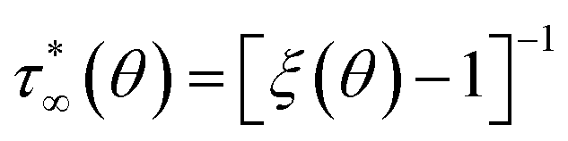

 or
or  .46 A general treatment of α-states would raise tough formal and numerical issues, falling beyond the experimental verification purposes of this work. In the next section, we thus limit ourselves to the neutral state
  (type C), which can be solved explicitly (e.g.
  ) to return
 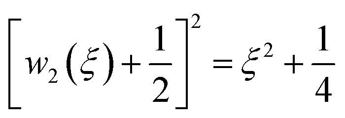 .45 The semi-heuristic position wα′(ξ) ≡ ξ, now with α′ ∈ [−1,1], would be rather convenient for an intuitive data analysis, but is formally inadequate for a model comparison, and is therefore disregarded.
 , in which ν is the kinematic viscosity and δt is a small time interval.47 The complementary error function, denoted by Φ−, quantifies the velocity fraction transmitted to the fluid upon shearing, and thus can be adopted for the evaluation of θ illustrated in Fig. 3 and explained in detail in Appendix 2.
 (i = d, dispersion; l, liquid) and P being a Gaussian function. This integral turns out to be well defined, as it is time-independent, and only depends upon ϕ through the ratio kd/ki:
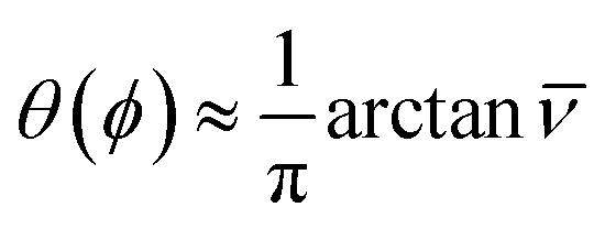
 . A boundary/cutoff value θa ≡ ϕa needs to be set independently, completing the definition of ξ = ξ(θ) in the previous relationships, with the requirement θ < ϕa, or:
 vs. ϕ was best fitted by means of each particle statistic, 1/α = 1 (A), ∞ (B), 2 (C) and the extracted model parameters are depicted in Table 1. Shear viscosity data vs. solid concentration were available for the system MWCNT/PC55 and fulfilled Eiler’s law,
  (e.g. ref. 56), where a large intrinsic viscosity value ([η] = 165) seems to be a feature of other carbon nanotube suspensions.57 Quemada’s model,

 ). Model parameters for α = 0 are in Table 1. Best fits with similar quality were also met in Ca3(PO4)2/H2O and Al2O3/C10H18 systems.
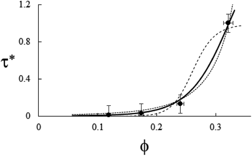
 . Reduced yield stress versus solid volume fraction for Si3N4/H2O. Lines and symbols are as in Fig. (4), and model parameters for
 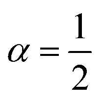 are in Table 1. Best fits with similar quality were also obtained in ZrO2/H2O.
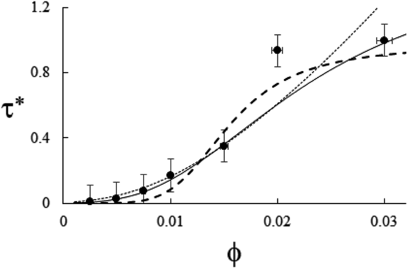


 in the limit of infinite dilution is anyway recovered upon ε → ∞. The actual values of stiffness parameters should guarantee a rather fast convergence since, for (A) and (B) distributions with
  and
and  :
:
 when ϕ → 0+.