 Open Access Article
Appraisal of Cu(II) adsorption by graphene oxide and its modelling via artificial neural network
Yumeng
Zhang
a,
Min
Dai
b,
Ke
Liu
c,
Changsheng
Peng
 *ab,
Yufeng
Du
a,
Quanchao
Chang
a,
Imran
Ali
ad,
Iffat
Naz
 *ef and
Devendra P.
Saroj
 *f
*f
aThe Key Lab of Marine Environmental Science and Ecology, Ministry of Education, College of Environmental Science and Engineering, Ocean University of China, Qingdao 266100, China. E-mail: cspeng@ouc.edu.cn; Tel: +86 532 66782011
bSchool of Environmental and Chemical Engineering, Zhaoqing University, Zhaoqing 526061, China
cDepartment of Mathematical Sciences, Tsinghua University, Beijing 100084, China
dDepartment of Agricultural Engineering, Bahauddin Zakariya University, Bosan Road, Multan 60800, Pakistan
eDepartment of Biology, Deanship of Educational Services, Qassim University, Buraidah 51452, Kingdom of Saudi Arabia. E-mail: iffatkhattak@yahoo.com; Tel: +966533897891
fDepartment of Civil and Environmental Engineering, University of Surrey, Guildford, UK. E-mail: d.saroj@surrey.ac.uk; Tel: +44(0) 1483686634
First published on 24th September 2019
Abstract
Graphene oxide (GO), as an emerging material, exhibits extraordinary performance in terms of water treatment. Adsorption is a process that is influenced by multiple factors and is difficult to simulate by traditional statistical models. Artificial neural networks (ANNs) can establish highly accurate nonlinear functional relationships between multiple variables; hence, we constructed a three-layered ANN model to predict the removal performance of Cu(II) metal ions by the prepared GO. In the present research work, GO was prepared and characterized by FT-IR spectroscopy, SEM, and XRD analysis techniques. In ANN modeling, the Levenberg–Marquardt learning algorithm (LMA) was applied by comparing 13 different back-propagation (BP) learning algorithms. The network structure and parameters were optimized according to various error indicators between the predicted and experimental data. The hidden layer neurons were set to be 12, and optimal network learning rate was 0.08. Contour and 3-D diagrams were used to illustrate the interactions of different influencing factors on the adsorption efficiency. Based on the results of batch adsorption experiments combined with the optimization of influencing factors by ANN, the optimum pH, initial Cu(II) ion concentration and temperature were anticipated to be 5.5, 15 mg L−1 and 318 K, respectively. Moreover, the adsorption experiments reached equilibrium at about 120 min. Combined with sensitivity analysis, the degree of influence of each factor could be ranked as: pH > initial concentration > temperature > contact time.
1. Introduction
Owing to the quick advancement in industrial and agricultural activities, the toxic metal ion contaminated water is being disposed into the natural water environment without appropriate treatment from both point and non-point pollutant sources. These toxic metal ions are not bio-degradable, and they can bio-accumulate in living beings and enter into our food chain.1 Copper (Cu) metal is a fundamental constituent for the living entities, and it also participates in the metabolic processes of the organisms. However, excessive intake of copper can cause damages to the liver, kidneys and other organs of the human body.2–4 A large part of the toxic Cu(II) ions in the environment come from different industrial activities (such as metallurgy, electroplating and tanning) without proper treatment, which is a serious environmental concern.5,6Therefore, to secure the biota (plants, animals and ecological environment), many researchers focus on the treatments of metal polluted wastewater via different methods and processes including adsorption, chemical precipitation, and electro-chemical methods.7–13 Among all water treatment technologies, adsorption is presumed to be effective and easy to carry out.14–16 In addition to this, novel and efficient adsorbents have been synthesized and applied in various fields of production and life. For example, nanomaterials are used in the field of environmental protection for controlling water and air pollution, and they are also used to store hydrogen energy in the new energy field. The discovery of new carbon nano-materials represented by carbon nanotubes, fullerenes and graphene has further boosted the progress of nanomaterial research.17–19 Graphene oxide (GO) is a special material with a monolayer of carbon atom thickness, and has different oxygenated functional groups on the surface and edge, making it a potentially effective adsorbent. The nature and magnitude of oxygenated functional groups of GO can be altered by the oxidation method, which may directly or indirectly influence the adsorption properties.20,21
Artificial neural network (ANN) is a computational model derived from the structure and function of the biological nervous system. The capability of an ANN model to study complex and non-linear processes enables it to accurately simulate human intuition in making conclusions.22 ANNs have been widely used to establish and optimize models in environmental studies such as environmental quality evaluation, analysis and prediction.23–26
The present work is concentrated on the preparation of GO and its adsorption properties of Cu(II). We constructed an ANN model to fit the adsorption results. The affecting factors were selected as the input variables of ANN, and the adsorption efficiency was the output variable. Compared to single-factor analysis, our neural network structure was more complex and required more parameters to learn. Therefore, the learning algorithm of the network, the structure of the covered layer and the learning rate were optimized to improve accuracy and robustness. The network after training was used to predict the corresponding removal efficiency under a combination of various factors, and we tested the validity by comparing predicted and experimental data.
2. Materials and methods
2.1 Chemicals and reagents
All the chemicals and reagents obtained from Sinopharm Chemical Reagent Company, including H2SO4, H3PO3, KMnO4, NaOH, CuSO4, H2O2 and HCl, were of analytical grade purity. The graphite powder (99.85% purity, particle size of 30 μm) was purchased from Damao Chemical Reagent Factory. The solutions of specific concentrations were obtained by dilution with de-ionized water.2.2 Fabrication and characterization of graphene oxide (GO)
With reference to the modified Hummers' method proposed by Marcano et al., the graphite powder was oxidized by KMnO4 in an acid environment, and then ultrasonically treated to obtain GO. In brief, graphene powder (1.5 g) was added to 200 mL of H2SO4/H3PO4 mixture (9![[thin space (1/6-em)]](https://www.rsc.org/images/entities/char_2009.gif) :
:![[thin space (1/6-em)]](https://www.rsc.org/images/entities/char_2009.gif) 1, v/v) and stirred at 300 rpm. While maintaining the temperature of the mixture below 10 °C, KMnO4 (6 g) was slowly added in portions and mixed evenly. After boiling in an oil bath at 50 °C for at least 12 h, the mixture was poured into 200 mL ice. 30% H2O2 solution was added drop by drop until the mixture turned golden. Afterwards, the material was centrifuged by HCl, ethanol and de-ionized water until the solution was neutral. The graphite oxide was exfoliated into GO by cell disruption, and the resulting suspension was freeze-dried to obtain the solid GO product.27
1, v/v) and stirred at 300 rpm. While maintaining the temperature of the mixture below 10 °C, KMnO4 (6 g) was slowly added in portions and mixed evenly. After boiling in an oil bath at 50 °C for at least 12 h, the mixture was poured into 200 mL ice. 30% H2O2 solution was added drop by drop until the mixture turned golden. Afterwards, the material was centrifuged by HCl, ethanol and de-ionized water until the solution was neutral. The graphite oxide was exfoliated into GO by cell disruption, and the resulting suspension was freeze-dried to obtain the solid GO product.27
The characteristics (such as morphology, elemental composition, presence of functional groups) of the as-prepared GO were examined using modern machinery including scanning electron microscope (SEM, EM6900, KYKY Technology Co., Ltd., China), powder X-ray diffractometer (XRD, D8 Advance, Bruker Ltd., Germany), and Fourier transform infrared spectroscope (FTIR-8000s, Shimadzu Ltd., Japan).
2.3 Batch adsorption study
We conducted batch adsorption experiments to investigate the influencing factors on the adsorptive efficiency of GO, including temperature, initial concentration of Cu(II) metal ions, pH and contact time. The adsorption experiments were carried out with 0.02 g of GO and 200 mL solution containing 5, 10, 15, 20, 25 and 30 mg L−1 of Cu(II) ions. The pH values of the suspensions were adjusted between 2.0–5.5 with 0.1 mol L−1 HCl or NaOH solution. This is because Cu(II) ions are the main species at pH < 5.5, and they might precipitate at higher pH, which will affect the adsorption results. The flasks were placed in a shaker with a speed of 150 rpm for predetermined time intervals (10, 30, 60, 90 and 120 min), and the mixture was separated by employing a 0.22 μm membrane filter. Thereafter, the concentration of Cu(II) metal ions was verified by an atomic absorption spectrophotometer (AA-7000, Shimadzu Ltd., Japan). To test for reproducibility, all trials were performed in triplicate and the means were used as the values of the input variables of the neural network. The efficiency of adsorption was calculated by the following equation: | (1) |
2.4 Artificial neural network (ANN)
The first neuron calculation model based on an electronic signal component was built in 1943.28 After several years of development, ANN models have been able to approximate multivariate continuous functions with appropriate network structure and learning algorithm at high speed. Taking the adsorption process as an example, the adsorption efficiency is determined by many factors, which makes it difficult to simulate the process through the traditional statistical models.29 However, ANN models have potential application in predicting the adsorption process due to their ability to establish a highly accurate nonlinear functional relationship between the variables.The Neural Network Toolbox of MATLAB (version 8.6.0) was utilized in the current research to build an ANN model. Aiming for a comprehensive evaluation of the adsorption capacity of the samples, we carried out adsorption experiments employing 90 different combinations of the four factors and took them as the input and adsorption efficiency as output values for our ANN model. Table 1 gives the range of input and output variables.
| Variables | Range of the parameter value |
|---|---|
| Input parameters | |
| pH | 2.0–5.5 |
| Initial concentration (mg L−1) | 5–30 |
| Temperature (K) | 298–318 |
| Contact time (min) | 10–120 |
![[thin space (1/6-em)]](https://www.rsc.org/images/entities/char_2009.gif) |
|
| Output parameters | |
| Adsorption efficiency (%) | 21.5–93.2 |
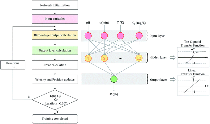
The parameters were optimized for constructing an ANN model, including hidden layer neurons, optimization algorithm, learning rate and the number of iterations. After the optimization, the ANN model was trained by the training set to carry out effective prediction. Given the input and output data, the connection weights and thresholds between neurons were adjusted as variables to lessen prediction errors.30 The predicted output of ANN model was linked with the trial data, and the biases were modified by calculating the error.31 When the error was less than the threshold (E(n) < ζ) or the number of iterations reached the upper limit (iterations > 100), the training process automatically stopped. The flowchart of ANN training process is shown in Fig. 1.
Based on the experimental data and network training steps, we constructed a three-layer network model. Signals were transmitted linearly and activated by processing unit function tan-sigmoid in the network.32 We compared 13 BP algorithms to find the most suitable algorithm. Then, based on the optimal BP algorithm, the optimal learning rate and structure of hidden layer were evaluated. Finally, the predicted data was compared with the desired data as the basis for judging our neural network learning results. The configuration of the model is also disclosed in Fig. 1.33
2.5 Recycling
To regenerate the adsorbent, the spent GO was placed in 0.1 mol L−1 HCl and shaken at 120 rpm for 12 h, then washed with de-ionized water until the pH was neutral. The regenerated GO was separated by centrifugation with a speed of 10![[thin space (1/6-em)]](https://www.rsc.org/images/entities/char_2009.gif) 000 rpm for 20 min, and then dried for reuse. This adsorption–desorption process was repeated 5 times.
000 rpm for 20 min, and then dried for reuse. This adsorption–desorption process was repeated 5 times.
3. Results and discussion
3.1 Characterization of graphene oxide (GO)
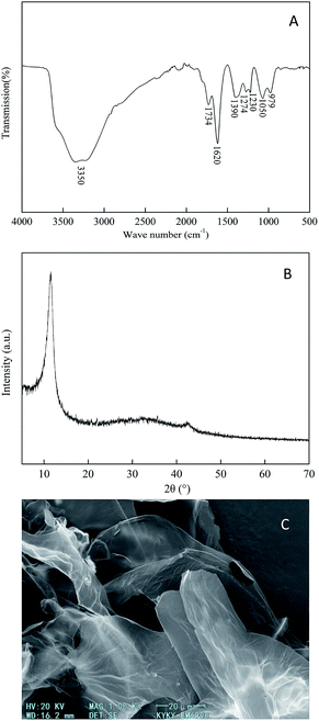
The prepared GO has many kinds of hydrophilic functional groups as displayed in Fig. 2a. There was a strong broad peak at 3350 cm−1, representing the O–H stretching vibration. The peaks at 1734, 1620, and 1390 cm−1 represented the stretching vibrations of C![[double bond, length as m-dash]](https://www.rsc.org/images/entities/char_e001.gif) O, C
O, C![[double bond, length as m-dash]](https://www.rsc.org/images/entities/char_e001.gif) C and C–OH functional groups, respectively. The peaks at 1274 and 1230 cm−1 resembled C–O vibrations, and the peak at 1050 cm−1 can be ascribed to the stretching vibration of the C–O–C functional group.34 The bending vibrational peak of the C–H bond appeared at 979 cm−1. The phase purity and crystalline nature of the GO samples were characterized using XRD analysis as shown in Fig. 2b. A significant diffraction peak appeared at the diffraction angle (2θ = 10.79°), with a corresponding interlayer distance of 0.819 nm, which is a characteristic peak of graphite oxide. The distinctive diffraction peak of graphite near 2θ = 26° did not appear, hinting that the oxidation process changed the crystal form of graphite into a new crystal structure. It can be seen from the SEM image (Fig. 2c) that the prepared GO has a layered structure with wrinkles on the surface, and the sheet has a large lateral dimension and a high aspect ratio.35,36
C and C–OH functional groups, respectively. The peaks at 1274 and 1230 cm−1 resembled C–O vibrations, and the peak at 1050 cm−1 can be ascribed to the stretching vibration of the C–O–C functional group.34 The bending vibrational peak of the C–H bond appeared at 979 cm−1. The phase purity and crystalline nature of the GO samples were characterized using XRD analysis as shown in Fig. 2b. A significant diffraction peak appeared at the diffraction angle (2θ = 10.79°), with a corresponding interlayer distance of 0.819 nm, which is a characteristic peak of graphite oxide. The distinctive diffraction peak of graphite near 2θ = 26° did not appear, hinting that the oxidation process changed the crystal form of graphite into a new crystal structure. It can be seen from the SEM image (Fig. 2c) that the prepared GO has a layered structure with wrinkles on the surface, and the sheet has a large lateral dimension and a high aspect ratio.35,36
3.2 Back-propagation algorithm
It is reported by Hornic that the feed forward neural network only needs one single hidden layer to fit any multivariate continuous function with arbitrary precision.37 We constructed a three-layer ANN model with input and output variables corresponding to four affecting factors and adsorption efficiency.Under the condition that the hidden layer contained 10 neurons, we selected the optimal training algorithm from 13 different algorithms by comparing the values of different parameters, such as root mean squared error (RMSE), correlation coefficient (R2), iteration number (IN) and optimal linear equation (OLE). The RMSE and R2 are calculated using eqn (2) and (3):
 | (2) |
 | (3) |
As shown in Table 2, the LMA with its smallest RMSE (0.0298) and fewer iterations was found to be the best of 13 BP learning algorithms, followed by the Bayesian regularization algorithm (BRA) with a RMSE of 0.0304. However, compared with LMA, which only needed 18 iterations of training, BRA took 100 iterations (iteration limit) to complete training.38 The RMSE of training and conjugate gradient algorithms such as gradient descent algorithm, one step secant algorithm, Fletcher–Powell algorithm were much larger than LMA.39 In addition to the properties of the algorithm itself, this may be due to the combinatorial properties and intrinsic link of the data set.
| Learning algorithms | Function | INa | RMSEb | R 2 c | Gradient | OLE1d | OLE2e |
|---|---|---|---|---|---|---|---|
| a IN, iteration number. b RMSE, root mean squared error. c R 2, correlation coefficient. d OLE1, the slope of optimal linear equation. e OLE2, the intercept of optimal linear equation. | |||||||
| Levenberg–Marquardt | trainlm | 18 | 0.0298 | 0.995 | 0.835 | 0.9914 | 0.6384 |
| Bayesian regularization | trainbr | 100 | 0.0304 | 0.973 | 0.417 | 0.9602 | 2.7892 |
| BFGS Quasi-Newton | trainbfg | 49 | 0.0489 | 0.975 | 0.606 | 0.9746 | 1.8732 |
| Resilient backpropagation | trainrp | 50 | 0.0499 | 0.943 | 0.885 | 0.9483 | 3.9410 |
| Scaled conjugate gradient | trainscg | 46 | 0.0407 | 0.940 | 0.812 | 0.9361 | 5.1059 |
| Conjugate gradient with Powell/Beale restarts | traincgb | 35 | 0.0493 | 0.971 | 0.395 | 0.9718 | 1.4668 |
| Fletcher–Powell conjugate gradient | traincgf | 21 | 0.1672 | 0.946 | 1.430 | 0.9632 | 2.7050 |
| Polak–Ribiére conjugate gradient | traincgp | 18 | 0.0744 | 0.912 | 0.678 | 0.8910 | 7.7585 |
| One step secant | trainoss | 17 | 0.1392 | 0.903 | 1.020 | 0.8266 | 13.7999 |
| Variable learning rate gradient descent | traingdx | 21 | 0.0794 | 0.555 | 1.080 | 0.6954 | 32.1423 |
| Gradient descent with momentum | traingdm | 36 | 0.2180 | 0.709 | 0.885 | 0.7289 | 21.5543 |
| Gradient descent | traingd | 100 | 0.1085 | 0.825 | 1.730 | 0.8791 | 8.6023 |
| Adaptive learning rate gradient descent | traingda | 91 | 0.1033 | 0.897 | 1.620 | 0.8662 | 11.2128 |
3.3 Optimization of the model structure
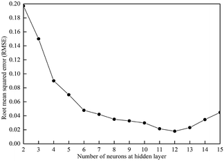
We optimized the structure and parameters of the ANN model based on the minimum RMSE between the projected and desired output data.40 The hidden neurons were defined to gradually increase from two, and the RMSE values of the neural networks were calculated. Because of the randomness of the neural network training, ANN training was performed at each learning rate for 200 times. Fig. 3 illustrates the correlation between the RMSE and the number of neurons in the hidden layer. RMSE tends to decrease first and then increase as the number of hidden layer neurons increases. If there were too few hidden layer neurons (<6), the weights could not meet the requirements for fitting the training data. However, too many neurons (>13) would increase the difficulty of the learning process, making it difficult to find a suitable combination of weights, and the learning results were rather poor.41,42 Based on the above analysis, the hidden layer neurons were set to 12 with a RMSE of 0.0179 in this study.3.4 Optimization of the learning rate
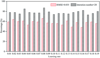
Learning rate is an important factor affecting the learning results of the neural network. If it is too high, the parameters of the neural network are difficult to converge. Conversely, if it is too low, it may be limited to the local optimal solution and fail to reach a better solution.43 The selection of learning rate is closely related to the structure and nature of learning data, so it cannot be determined before training. Fig. 4 shows the learning results with 12 hidden neurons with LMA.Due to the randomness of the learning process, we performed training for 200 times at each learning rate and counted the ratio of iterations less than 20 and RMSE less than 0.035. The ratio of learning iterations less than 20 was generally around 80%, and the ratio was the highest when the learning rate was 0.08, reaching 87%. RMSE was used as an important indicator for evaluating the learning rate because it was related to the training results.44 At a learning rate of 0.08, the ratio of RMSE less than 0.035 reached a maximum of 66.5%. Therefore, the learning rate selected in this study was 0.08.
3.5 Training process
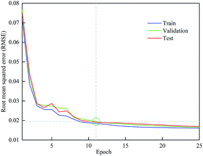
In this work, 70%, 15% and 15% of the experimental data were allocated to the training, validation and test set, respectively. Fig. 5 shows the RMSE of different data set with a learning rate of 0.08. The training stopped at 11 iterations because the errors between the predicted and experimental data for all three training groups were within the required tolerance. After that, the gap between the training and test RMSE started to increase, which might lead to over-fitting. Therefore, when the optimum iteration number was 11, the training, validation and test RMSE were 0.0185, 0.0194 and 0.0191, respectively.3.6 Sensitivity analysis
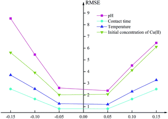
In this study, the sensitivity analysis of the proposed ANN model was conducted to judge the degree of influence of each input factor on the adsorption efficiency using the mean impact value (MIV) method. The values of each input variables were increased and reduced by 1%, 5%, and 10% respectively, while other factors were fixed, and the RMSE of corresponding output variables were calculated through the ANN model.45 The sensitivity analysis helps to determine which parameters are the key drivers of the model results so that the factor that has the greatest influence on the adsorption efficiency can be obtained.As shown in Fig. 6, the sensitivity of the pH is much greater than that of the other factors, both in terms of the RMSE values and the ranges of the output variables varying with the input variables. When the pH of the input variable was reduced by 15%, the RMSE reached 8.53. It can also be seen from the original experimental data that the pH had the foremost effect on the results, which was consistent with the analysis in Section 3.7.46 The input variable of contact time was the least influential factor. When the contact time was reduced by 15%, the RMSE of the output variable was only 2.51. It was confirmed by the original experimental data that the adsorption efficiency tended to be flat after 90 minutes and reached equilibrium at approximately 120 minutes. The influence of temperature was slightly larger than that of time but far less than that of pH. When the temperature was reduced by 15%, the RMSE of the output variable was 3.70. The higher RMSE value of the output variable indicated that the value of the initial concentration was greater than that of the proportional decreased. This was because the effects of factors other than the initial concentration tended to be stable as the values increased.47
3.7 Contour and three-dimensional diagrams for the effects of adsorption properties
As seen in Fig. 7, the effects of the four factors are comprehensive and not independent of one another. Therefore, we analyzed the combination of different factors, rather than separately analyzing the influence of one factor on the adsorption results while fixing all the other factors. After adsorption equilibrium, the influences of pH and temperature on adsorption efficiency are independent of time because prolonged adsorption time no longer affects the adsorption results. However, the increase in initial concentration leads to a continuous decrease in efficiency, which is different from contact time (also mentioned in Section 3.6). Therefore, the interaction between initial concentration and other factors needs to be focused on.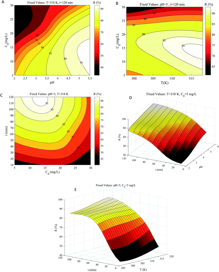 | ||
| Fig. 7 Contour and three-dimensional diagrams for interactive effects of (A) pH × C0; (B) T × C0; (C) C0 × t; (D) pH × t; (E) T × t on R. | ||
The interaction of pH and initial concentration on copper removal efficiency was studied at a fixed temperature and time (Fig. 7a). The effect of pH on adsorption efficiency is strictly monotonically proportional, whereas the initial concentration is monotonically inversely proportional though not rigorous. It was reported that metal ions occupied the adsorption sites more quickly at lower concentrations. However, at pH ranging from 4.5 to 5.5, the removal efficiency increased slightly and then decreased with the concentration boosting from 5 to 20 mg L−1. This may be because GO was saturated at an initial concentration above 15 mg L−1. At low pH (2.0–3.5), the influence of high concentration on adsorption efficiency was lesser than that at a higher pH (4.5–5.5). The pH of the solution can alter the presence and magnitude of Cu(II) metal ions, the surface electrical properties of materials, and the interaction between the materials and the ions.48 Excessive H+ adsorbs on GO at lower pH, occupying the adsorption sites of Cu(II) metal ions, while a higher pH value enhances the attraction between copper metal ions and the negative charge on the GO surface.49,50 Under the conditions of fixed temperature and time, a minimum adsorption efficiency of 33.2% was obtained at pH = 2.0 and an initial concentration of 30 mg L−1; the maximum efficiency of 93.2% was obtained at pH = 5.5 and an initial concentration of 15 mg L−1.
At fixed pH and adsorption time, the interaction of temperature and initial concentration is depicted in Fig. 7b. The increasing temperature and decreasing concentration enhanced copper removal, and the Cu(II) metal ion concentration has a greater influence. The adsorptive efficiency was about 85.4% at low concentrations (5–23 mg L−1) and low temperatures (293–303 K). When the temperature rose above 303 K, the adsorption efficiency could exceed 90%, suggesting that the adsorption method may be endothermic. In the range of 23 to 30 mg L−1, the minimum efficiency reached 58.1% at low temperatures and 71.3% at high temperatures, which meant that an appropriate initial concentration was more conducive to higher removal efficiency than the temperature (consistent with Section 3.6).
Fig. 7c illustrates the interaction between concentration and time at a fixed temperature of 318 K and pH of 5.5. The strong attraction between GO and Cu(II) metal cations led to the rapid increase of adsorption efficiency at the initial stage (10–45 min).51 After 90 minutes, the adsorption rate tended to be flat and finally reached equilibrium for all initial concentration conditions at approximately 120 minutes. When the concentration was 5–20 mg L−1, the efficiency was substantially over 90% after 120 min.52 Minimum efficiency of 43.2% was obtained for a contact time of 10 min and an initial concentration of 30 mg L−1. The maximum adsorption efficiency of 93.2% was acquired at the initial concentration of 15 mg L−1 for the contact time of 120 min. Based on the analysis of Fig. 7a–c, the degree of influence of the related variables is ranked as: pH > initial concentration > temperature, which is consistent with Section 3.6.
Fig. 7d shows the interactive effects of pH and contact time on adsorption efficiency. With the increase of pH and adsorption time, the adsorption efficiency first increased greatly and then flattened.53 At pH = 2, the lowest and highest adsorption efficiencies were 23.3% and 74.8%, which were obtained at contact times of 10 and 120 min, respectively. At pH = 5.5, the lowest and highest adsorption efficiencies were 50.7% and 93.0%, which were obtained at a contact time of 10 and 120 min, respectively. This may be due to the promotion of faster adsorption of Cu2+ at higher pH. Although the efficiency interval was different, the efficiency gap was almost identical under the same contact time.
The interaction of temperature and contact time on adsorption efficiency was also investigated (Fig. 7e). Within the temperature range of 298 to 318 K, the adsorption efficiency increased from 42.2 to 48.2% and 83.9 to 93.0% for the contact time of 10 and 120 min, respectively. Compared with Fig. 7d, the effect of pH was greater than that of the temperature, but the effects of pH and temperature are roughly the same (both positive correlations).54 To compare the effects of different factors, we normalized the input data of the network. Although the adsorption efficiency varied greatly with the contact time before the equilibrium, the adsorption was almost unaffected by the contact time after the equilibrium at 120 min, making contact time the least sensitive factor of the whole.55
3.8 Desorption and regeneration of GO
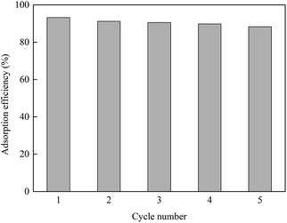
The adsorption capacity and desorption performance are two important indicators to evaluate the adsorbents. The desorption experiment was carried out using 0.1 mol L−1 HCl because H+ competes with Cu2+ on the GO surface for adsorption sites. As shown in Fig. 8, after five adsorption–desorption cycles, the adsorption efficiency still reached 87.9%, which was about 5.3% lower than that of the initial adsorption experiment. It can be seen that GO has good reproducibility and has a promising future as a water treatment adsorbent.4. Conclusions
We successfully prepared and characterized GO for the adsorption of Cu(II) metal ions. The findings indicated that the maximum percentage of Cu(II) metal ion removal reached 93.2% at the concentration of 15 mg L−1, temperature of 318 K, pH of 5.5, and the adsorption experiments reached equilibrium at about 120 min. The desorption experiments indicated that the prepared GO can be easily regenerated by a HCl solution.In this work, an ANN model was built to study the various factors related to the adsorption process. Signals were transmitted linearly and activated by processing unit function tan-sigmoid in a three-layer ANN. To make the model more suitable for the data, the structure and parameters of the neural network were optimized by comparing the evaluation index, including RMSE. The number of iterations and RMSE of 13 different BP algorithms were compared comprehensively, and LMA was found to be the best algorithm. The optimal hidden layer neurons were 12 with the minimum RMSE of 0.0179. The learning rate selected in this study was 0.08 with the ratio of RMSE of less than 0.035 reaching a maximum of 66.5%, and the training was stopped at 11 iterations.
The contour and three-dimensional diagrams showed that the removal efficiency was boosted with an increase in the temperature, pH, contact time, and decrease in the initial concentration. According to the diagrams and sensitivity analysis, the influence degree of each factor on the adsorption efficiency was: pH > initial concentration > temperature > contact time. Moreover, the RMSE of the output variable that increased the value of initial concentration was greater than that of the proportional decreased. The explanation is that the efficiency decreased with the increasing concentration and tended to be stable with the increase of other factors. In brief, the ability of an ANN model to learn and summarize complex and non-linear processes can provide us with a new perspective for the adsorption process.
Conflicts of interest
The authors declare no conflict of interest.Acknowledgements
The authors gratefully acknowledge the economic support from the Zhaoqing Science and Technology Project (2018N006) and the State Key Laboratory of Environmental Criteria and Risk Assessment (SKLECRA2013FP12). Dr Saroj's contribution to this paper was supported by InRoot and Water-Food scoping projects at University of Surrey studying wastewater treatment for reuse as part of STFC Food Security Network led by the University of Manchester [Grant number ST/P003079/1].References
- D. Núñez, J. A. Serrano, A. Mancisidor, E. Elgueta, K. Varaprasad, P. Oyarzún, R. Cáceres, W. Ide and B. L. Rivas, RSC Adv., 2019, 9, 22883–22890 RSC.
- M. R. Awual, M. M. Hasan, M. A. Khaleque and M. C. Sheikh, Chem. Eng. J., 2016, 288, 368–376 CrossRef CAS.
- X. Li, Y. Liu, C. Zhang, T. Wen, L. Zhuang, X. Wang, G. Song, D. Chen, Y. Ai, T. Hayat and X. Wang, Chem. Eng. J., 2018, 336, 241–252 CrossRef CAS.
- K. Russell, L. K. Gillanders, D. W. Orr and L. D. Plank, Eur. J. Clin. Nutr., 2018, 72, 326–331 CrossRef CAS.
- S. A. Al-Saydeh, M. H. El-Naas and S. J. Zaidi, J. Ind. Eng. Chem., 2017, 56, 35–44 CrossRef CAS.
- P. Liu, P. F. Borrell, M. Božič, V. Kokol, K. Oksman and A. P. Mathew, J. Hazard. Mater., 2015, 294, 177–185 CrossRef CAS.
- H. Peng, P. Gao, G. Chu, B. Pan, J. Peng and B. Xing, Environ. Pollut., 2017, 229, 846–853 CrossRef CAS.
- P. Liu, K. Oksman and A. P. Mathew, J. Colloid Interface Sci., 2016, 464, 175–182 CrossRef CAS PubMed.
- A. M. Ghaedi, M. Ghaedi, A. Vafaei, N. Iravani, M. Keshavarz, M. Rad, I. Tyagi, S. Agarwal and V. K. Gupta, J. Mol. Liq., 2015, 206, 195–206 CrossRef CAS.
- J. Rodrigues Pires da Silva, F. Merçon, C. Manoel Guimarães Costa and D. Radoman Benjo, Desalin. Water Treat., 2016, 41, 19466–19474 CrossRef.
- M. Kumar, R. Shevate, R. Hilke and K. Peinemann, Chem. Eng. J., 2016, 301, 306–314 CrossRef CAS.
- N. Z. KassimShaari, N. A. Sulaiman and N. A. Rahman, J. Environ. Chem. Eng., 2019, 7, 102845 CrossRef.
- S. Caprarescu, M. C. Corobea, V. Purcar, C. I. Spataru, R. Ianchis, G. Vasilievici and Z. Vuluga, J. Environ. Sci., 2015, 35, 27–37 CrossRef CAS.
- M. Tanzifi, M. T. Yaraki, A. D. Kiadehi, S. H. Hosseini, M. Olazar, A. K. Bharti, S. Agarwal, V. K. Gupta and A. Kazemi, J. Colloid Interface Sci., 2018, 510, 246–261 CrossRef CAS.
- W. Wang, J. Yu, X. Yang, B. Yu and X. Cai, J. Chem. Technol. Biotechnol., 2019, 94(10), 3333–3343 CrossRef CAS.
- M. Xia, Z. Chen, Y. Li, C. Li, N. M. Ahmad, W. A. Cheema and S. Zhu, RSC Adv. , 2019, 9, 2941–2953 RSC.
- M. Moghaddari, F. Yousefi, M. Ghaedi and K. Dashtian, Ultrason. Sonochem., 2018, 42, 422–433 CrossRef CAS.
- J. Xu, Z. Cao, Y. Zhang, Z. Yuan, Z. Lou, X. Xu and X. Wang, Chemosphere, 2018, 195, 351–364 CrossRef CAS.
- S. Dang, Q. Zhu and Q. Xu, Nat. Rev. Mater., 2018, 3, 1–14 CrossRef.
- K. Krishnamoorthy, M. Veerapandian, K. Yun and S. J. Kim, Carbon, 2013, 53, 38–49 CrossRef CAS.
- P. Tan, Q. Bi, Y. Hu, Z. Fang, Y. Chen and J. Cheng, Appl. Surf. Sci., 2017, 423, 1141–1151 CrossRef CAS.
- G. Villarrubia, J. F. De Paz, P. Chamoso and F. D. la Prieta, Neurocomputing, 2018, 272, 10–16 CrossRef.
- I. Ali, O. M. L. Alharbi, Z. A. Alothman, A. Y. Badjah, A. Alwarthan and A. A. Basheer, J. Mol. Liq., 2018, 250, 1–8 CrossRef CAS.
- F. Yang, H. Cho, H. Zhang, J. Zhang and Y. Wu, Energy Convers. Manage., 2018, 164, 15–26 CrossRef.
- E. S. Elmolla, M. Chaudhuri and M. M. Eltoukhy, J. Hazard. Mater., 2010, 179, 127–134 CrossRef CAS PubMed.
- M. HemmatEsfe, M. Reiszadeh, S. Esfandeh and M. Afrand, Phys. A, 2018, 512, 731–744 CrossRef CAS.
- D. C. Marcano, D. V. Kosynkin, J. M. Berlin, A. Sinitskii, Z. Sun, A. Slesarev, L. B. Alemany, W. Lu and J. M. Tour, ACS Nano, 2010, 4, 4806–4814 CrossRef CAS.
- W. S. McCulloch and W. Pitts, Bull. Math. Biol., 1943, 52(99–115), 73–97 Search PubMed.
- A. Asfaram, M. Ghaedi, M. H. A. Azqhandi, A. Goudarzi and M. Dastkhoon, RSC Adv., 2016, 6, 40502–40516 RSC.
- A. M. Ghaedi and A. Vafaei, Adv. Colloid Interface Sci., 2017, 245, 20–39 CrossRef CAS.
- I. Aljarah, H. Faris and S. Mirjalili, Soft Computing, 2018, 22, 1–15 CrossRef.
- R. Karimi, F. Yousefi, M. Ghaedi and K. Dashtian, Chemom. Intell. Lab. Syst., 2016, 159, 127–137 CrossRef CAS.
- Z. Ye and M. K. Kim, Sustain. Cities Soc., 2018, 42, 176–183 CrossRef.
- K. Yang, B. Chen, X. Zhu and B. Xing, Environ. Sci. Technol., 2016, 50, 11066–11075 CrossRef CAS.
- S. Stankovich, D. A. Dikin, G. H. B. Dommett, K. M. Kohlhaas, E. J. Zimney, E. A. Stach, R. D. Piner, S. T. Nguyen and R. S. Ruoff, Nature, 2006, 442, 282–286 CrossRef CAS.
- D. R. Dreyer, S. Park, C. W. Bielawski and R. S. Ruoff, Chem. Soc. Rev., 2010, 39, 228–240 RSC.
- K. Hornic, Neural Netw., 1989, 5, 359–366 CrossRef.
- M. Kayri, Math. Comput. Appl., 2016, 21, 20 Search PubMed.
- N. Andrei, J. Comput. Appl. Math., 2016, 292, 83–91 CrossRef.
- M. Tanzifi, S. H. Hosseini, A. D. Kiadehi, M. Olazar, K. Karimipour, R. Rezaiemehr and I. Ali, J. Mol. Liq., 2017, 244, 189–200 CrossRef CAS.
- M. Dastkhoon, M. Ghaedi, A. Asfaram, M. H. AhmadiAzqhandi and M. K. Purkait, Chem. Eng. Res. Des., 2017, 124, 222–237 CrossRef CAS.
- M. Tanzifi, M. TavakkoliYaraki, M. Karami, S. Karimi, A. DehghaniKiadehi, K. Karimipour and S. Wang, J. Colloid Interface Sci., 2018, 519, 154–173 CrossRef CAS.
- K. O. Stanley, J. Clune, J. Lehman and R. Miikkulainen, Nat. Mach. Intell., 2019, 1, 24–35 CrossRef.
- S. Chatterjee, S. Sarkar, S. Hore, N. Dey, A. S. Ashour and V. E. Balas, Neural Comput. Appl., 2017, 28, 2005–2016 CrossRef.
- M. Fouladgar, M. Beheshti and H. Sabzyan, J. Mol. Liq., 2015, 211, 1060–1073 CrossRef CAS.
- L. Cui, Y. Wang, L. Gao, L. Hu, L. Yan, Q. Wei and B. Du, Chem. Eng. J., 2015, 281, 1–10 CrossRef CAS.
- T. Jiang, W. Liu, Y. Mao, L. Zhang, J. Cheng, M. Gong, H. Zhao, L. Dai, S. Zhang and Q. Zhao, Chem. Eng. J., 2015, 259, 603–610 CrossRef CAS.
- W. Peng, H. Li, Y. Liu and S. Song, Appl. Surf. Sci., 2016, 364, 620–627 CrossRef CAS.
- N. Bakhtiari and S. Azizian, J. Mol. Liq., 2015, 206, 114–118 CrossRef CAS.
- J. Deng, Y. Liu, S. Liu, G. Zeng, X. Tan, B. Huang, X. Tang, S. Wang, Q. Hua and Z. Yan, J. Colloid Interface Sci., 2017, 506, 355–364 CrossRef CAS.
- M. Wei, H. Chai, Y. Cao and D. Jia, J. Colloid Interface Sci., 2018, 524, 297–305 CrossRef CAS.
- S. H. Park, H. J. Cho, C. Ryu and Y. Park, J. Ind. Eng. Chem., 2016, 36, 314–319 CrossRef CAS.
- G. Sheng, C. Huang, G. Chen, J. Sheng, X. Ren, B. Hu, J. Ma, X. Wang, Y. Huang, A. Alsaedi and T. Hayat, Environ. Pollut., 2018, 233, 125–131 CrossRef CAS.
- J. Wang and B. Chen, Chem. Eng. J., 2015, 281, 379–388 CrossRef CAS.
- A. L. P. Xavier, O. F. H. Adarme, L. M. Furtado, G. M. D. Ferreira, L. H. M. Da Silva, L. F. Gil and L. V. A. Gurgel, J. Colloid Interface Sci., 2018, 516, 431–445 CrossRef CAS.
| This journal is © The Royal Society of Chemistry 2019 |

