An autonomous microreactor platform for the rapid identification of kinetic models

Abstract

An autonomous flow microreactor platform was developed that was able to conduct reaction experiments and measure the outlet reactant and product concentrations using HPLC without user supervision. The platform performed unmanned kinetic experiments with the aim of precisely estimating the parameters of a kinetic model for the esterification between benzoic acid and ethanol catalysed by sulfuric acid. The capabilities of the autonomous platform were demonstrated on three different experimental scenarios: 1) performing steady-state experiments, where the experimental reaction conditions were pre-defined by the user; 2) performing steady-state experiments, where the conditions were optimised online by Model-Based Design of Experiments (MBDoE) algorithms, with the aim of improving parameter precision; 3) executing transient experiments, where the conditions were pre-selected by the user. For the steady-state experiments, the platform automatically performed online parameter estimation and MBDoE with a pre-selected kinetic model. It was demonstrated that a campaign of steady-state experiments designed using online MBDoE algorithms led to more precise parameter estimates than a campaign of experiments designed by the traditional factorial design. Transient experiments were shown to expedite kinetic parameter estimation and use less reagents than campaigns of steady-state experiments, as it was no longer necessary to wait for the system to reach steady-state. In general, the transient experiments offered less precise parameter estimates than the steady-state campaigns, however the experiments could be completed in just 2 h instead of the 8 h required for a campaign of steady-state experiments.

---

Introduction

A reliable reaction kinetic model provides many advantages for a chemical process. Most notably it allows for improved design of the reactor and the process control system, as well as enabling process optimisation, hence potentially making a process greener, safer and more profitable. However, obtaining a kinetic model can be a challenging task which is time consuming and expensive. The two major difficulties in obtaining a kinetic model are identifying the true or most useful model structure from alternative candidate models, and then obtaining statistically satisfactory parameter estimates for the model parameters which are often highly correlated.^1,2 Due to these obstacles it is necessary to spend large amounts of time performing experiments, and some of these experiments, if poorly designed, will not significantly improve the model identification process and hence will be a waste of time and resources.

In recent years the development of flow reactors compatible with both online analysis equipment and automated control algorithms has begun to modernise the way in which chemical kinetics are obtained. Traditionally kinetics are obtained in batch, which while having the advantage of providing multiple data points per experiment, may be limited by heat and mass transfer. In comparison, the development of flow microreactors with superior rates of heat and mass transport and improved safety^3–7 enable isothermal kinetic studies.^5,8–10 Flow reactors are now often combined with online analysis to provide data-rich experimental platforms. Online flow analysis methods reported in the literature include GC,^11–14 HPLC,^15–23 MS,^16,23–26 UV,¹³ IR,^27–32 Raman,^33,34 X-ray absorption spectroscopy²⁸ and NMR³⁵ as well as viscosity measurements.³⁶ Additionally, many flow reactors are now being programmed to perform experiments automatically, while collecting experimental data without user supervision. These automated reactor systems have already been successfully applied to reaction monitoring^11,16 and high throughput continuous and discrete variable screening for reaction discovery and optimisation.^26,37,38 In addition to performing steady-state experiments, flow reactors also present opportunities to perform transient experiments,^39,40 either by ramping^22,29,31 or introducing pulses⁴¹ or step changes⁴² in variables such as temperature and flowrate, which can reduce the time and materials required to generate sufficient data for kinetic identification.

One of the most exciting developments in flow chemistry in recent years is the emergence of closed loop systems.^43–45 These systems consist of i) an automated reactor ii) an online measurement system and iii) a reactor control system implementing an algorithm for Design of Experiments (DoE) which uses information gathered from the online measurement system. A wide variety of DoE algorithms can be implemented in closed loop systems depending on the objectives of the experimental activity. The DoE algorithms can be broadly divided into two categories, black-box optimisation and model based optimisation. In black-box optimisation, a model of the reactor is not required and the objective is often to maximise yield or conversion. There are a large number of black-box closed loop systems reported in the literature, and they are often called “self-optimising reactors”.^{12–14,17,25,30,32,35,45–50} Some of the most impressive applications of self-optimising reactors include the automation of a multistep sequence including reaction and separation steps²³ and the use of multiple objective functions where an optimal compromise between two competing variables (such as profitability and environmental impact) has to be identified.⁵¹ However, while the self-optimising reactors offer many advantages, they are normally of little value in developing a kinetic model, as the experiments are usually performed only in the region around the optimum operating point. For this reason black-box optimisation is not pursued in this work. In comparison, MBDoE is much more suited to developing kinetic models, which are more useful for scale-up purposes than a knowledge of an optimum operating point in a lab scale reactor. While MBDoE can be targeted to model discrimination,^2,19,52,53 (the identification of the most suitable model from a list of candidate models), this was not pursued in this work as a single model structure is assumed to be true. Instead this work takes advantage of MBDoE for the precise estimation of parameters.^2,54–57 While there are numerous successful examples of the application of MBDoE for precise parameter estimation in the literature,^2,58–63 the online application of MBDoE is much less common. To the best of the authors' knowledge there exist only few publications where online MBDoE has been applied to chemical kinetic models.^13,19,64,65

The aim of this work is to develop an autonomous reactor platform for rapid kinetic studies that can be applied to a wide range of reactions. The autonomous platform is designed to be able to conduct both transient experiments and steady-state experiments. In the case where a model structure is not known in advance, this autonomous platform is able to conduct transient experiments or a set of steady-state experiments chosen in advance by the user. However, in cases where the user provides the platform with a pre-selected kinetic model, then it is able to perform either automated parameter estimation or online MBDoE for sequential steady-state experiments with the aim of obtaining the most precise parameter estimates possible. The automation of kinetic experiments in this way not only leads to more efficient use of lab resources, but it can free up time of highly trained researchers allowing them to focus on more intellectually demanding tasks, such as designing new set-ups or analysing data.

Materials and methods

Experimental set-up

The autonomous platform was validated using the case study of benzoic acid esterification with ethanol, with sulfuric acid as a homogenous catalyst, shown in eqn (1).

Benzoic Acid + Ethanol ⇄ Ethyl Benzoate + Water C₆H₅COOH + C₂H₅OH ⇄ C₆H₅COOC₂H₅ + H₂O (1)

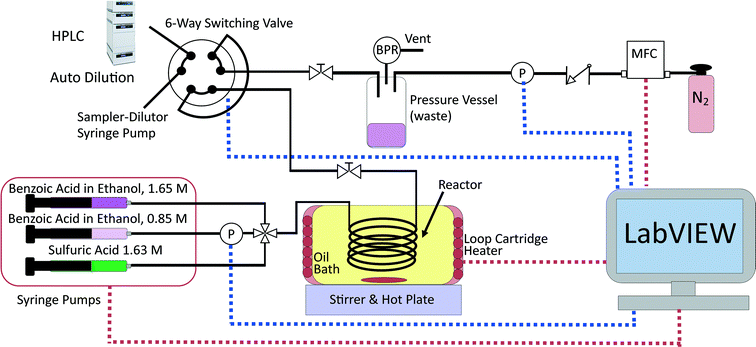
This reaction was chosen due to its simplicity as a homogenous reaction. It is also extremely slow at room temperature, hence the reaction can be stopped by simple cooling without requiring chemical quenching.⁶⁶ The experimental set-up is shown in Fig. 1 and included a reactor which was a 2 m long 250 μm internal diameter (i.d.) PEEK tube (Agilent) placed in a stirred oil bath heated by a rope heater (OMEGALUX FGR 6 foot length, 250 W). The small diameter ensured the reactor behaved as a plug flow reactor for the liquid flowrates used (5–100 μL min⁻¹); the vessel dispersion number, N_L, was estimated to be <0.006 for all conditions studied (see ESI†), which was <0.01, the commonly considered criterion for the validity of the plug flow assumption.⁶⁷ The small diameter tubing also provided high rates of heat transfer, so that the reaction mixture reached reaction temperature (at reactor inlet) or room temperature (at reactor outlet) very quickly when the tubing entered and left the oil bath (see heat transfer calculations in the ESI†). The reaction rate has been found to be negligible at room temperature and this allowed the reaction to be quenched simply by cooling, as the tubing left the oil bath and was exposed to air. The reaction was shown not to occur without the presence of the sulfuric acid catalyst; this allowed the reagents to be pre-mixed in 5 ml glass syringes (5 mL mid pressure, Cetoni) before use. Two syringes filled with different concentrations of benzoic acid in ethanol (0.85 and 1.65 M) were used to allow control of the feed concentration at any value between these two concentrations by adjusting the relative flowrates of the syringe pumps (neMESYS, low pressure module, Cetoni). The sulfuric acid concentration was kept constant at 0.163 M in the reactor by pumping a 1.63 M sulphuric acid in water solution at a flowrate 10% of the value of the total inlet flowrate. The reagents were mixed at a PEEK four-way junction with a 0.5 mm through-hole (UpChurch) and flowed through 30 cm of 250 μm tubing before reaching the oil bath, hence ensuring they were well mixed before entering the reactor (see ESI† for further mixing calculations). Due to the low boiling point of ethanol and the high reaction temperatures required to produce a reasonable rate of reaction, the system was pressurised to 6 barg to keep the reactants in the liquid phase for temperatures up to 140 °C. This was achieved by pressurising the product collection vessel with nitrogen gas from a mass flow controller (SLA mass flow controller, Brooks) and using a back-pressure regulator (Swagelok K series, 250 psig) set to the desired pressure. A pressure sensor (Honeywell 40PC, 250 psig) was connected inline with the pressure vessel to provide an accurate pressure reading of the back-pressure and a second pressure sensor (Zaiput Hastelloy, 300 psi, ≈10 μL dead volume) was placed inline in the low concentration benzoic acid line to measure the upstream pressure and hence the pressure drop, which was typically <0.2 bar. The product collection vessel consisted of a centrifuge tube (Corning 50 mL) with a custom made PEEK holder with three ports designed to withstand high pressure.

Fig. 1 Experimental set-up for the esterification of benzoic acid with ethanol using sulfuric acid as a homogenous catalyst. Red dashed lines indicate LabVIEW controls the equipment, blue dashed lines indicate LabVIEW reads the measurement from the equipment. BPR: back-pressure regulator; MFC: mass flow controller; P: pressure sensor.

The reactor outlet was connected to the 6-way switching valve of an automatic sampler-dilutor (Syrris, Asia Sampler and Dilutor), which was connected to an HPLC (Jasco LC-4000) for online concentration measurement. The sampler-dilutor had a 10 μL sample loop and a large dilution factor of 250 was used to protect the column from the sulfuric acid. The HPLC column was a 250 mm long, 4.6 mm i.d. ODS hypersil column with 5 μm particle size (Thermo Fisher Scientific). The HPLC method used 1.25 mL min⁻¹ of mobile phase consisting of 40% water and 60% acetonitrile by volume and the analysis lasted 7 min. The oven was held constant at 30 °C and a UV detector at 274 nm was used for quantification of the benzoic acid and ethyl benzoate concentrations. The standard deviation of the measurement error was found from repeated identical experiments to be 0.03 M for the benzoic acid concentration and 0.0165 M for the ethyl benzoate concentration. These standard deviations were used in the constant variance model for both parameter estimation and MBDoE. The measurement error was attributed to the combination of errors in the HPLC and the sampler-dilutor.

Statistical tools for model development and validation

Parameter estimation

Our model comprised of a set of equations, a vector of N_θ non-measurable parameters θ, state variables x and inputs u, that can be used to predict the behaviour of the system and hence can predict experimentally measurable values ŷ:

ŷ = f(x, u, θ) (2)

The non-measurable parameters θ, were the two Arrhenius parameters KP1 and KP2 (see later), while the inputs u, were the three control variables: temperature, flowrate and inlet concentration and the two fixed variables: pressure and sulfuric acid concentration. The state variables x were the reactant and product concentrations along the length of the reactor and y represented the measured concentrations of benzoic acid and ethyl benzoate at the reactor outlet. For parameter estimation, experimental measurements were used to identify the values of the non-measurable parameters θ, in a model. In a system where N_exp experiments are conducted with each experiment consisting of N_m measurements, then for the i^th experiment and j^th measurement the i,j^th residual ρ_ij, is defined as the difference between the model predicted value ŷ_ij and the experimentally measured value y_ij:

ρ_ij = y_ij − ŷ_ij (3)

Parameter estimation was conducted using the maximum likelihood principle, which assumes that i) the model structure is correct (the correct kinetic rate laws and reactor models are used) ii) there is no error associated with the experimental inputs u and iii) the residuals are caused by measurement errors, which are assumed to be normally distributed with a mean of 0 and a standard deviation σ_ij.^2,68 With these assumptions, parameter estimation was performed by finding the set of parameter values [small straight theta, Greek, circumflex], which maximised the log likelihood function (referred to as the objective function Φ(θ)), shown in eqn (4).

Goodness of fit

After completing the parameter estimation, it is necessary to assess the fitting of the model. Data fitting is a measure of how well a model describes the real physical system. If all the assumptions are correct (correct model structure, no error in the inputs and randomly distributed measurement errors with a mean of 0 and standard deviation σ), then the residuals should be randomly distributed with a mean of 0 and a standard deviation equal to their respective measurement error standard deviations. Therefore, by studying the residuals it is possible to identify if the previous assumptions are true or not. This is done using the χ² test which measures the fitting quality by comparing the χ² value, computed using eqn (5), to the χ² reference value at a 95% confidence level for the given number of degrees of freedom (degrees of freedom = N_exp × N_m − N_θ).

If all the previous assumptions are true, there is a 95% probability that the χ² value will be less than the χ² reference value. Most commonly, and in this work, it is assumed that the measurement error is accurately known and the experimental inputs are assumed to be well controlled, therefore whenever the χ² value is greater than the reference value, the model is rejected as being incompatible with the data collected. In this work, the measurement error was the standard deviation of repeated experiments.

Parameter accuracy and precision

After finding a suitable model that satisfies the χ² test it is necessary to assess the quality of the parameter estimation. In parameter estimation the two most important quantities are accuracy and precision. Accuracy is how close the parameter estimate is to the true value, however in real situations the true value is unknown and therefore it is not possible to estimate accuracy, except in simulated case studies when the true parameters are known. As parameter estimates are themselves randomly distributed variables, they have a standard deviation and precision, which describes if the same experiments and parameter estimation procedure were repeated multiple times, how spread out the resulting parameter estimates would be. A graphical explanation of accuracy and precision is included in the ESI.† The parameter precision is calculated from the covariance matrix V_θ, which can be approximated (using the first term Taylor expansion) as the inverse of the negative Hessian of the objective function as shown in eqn (6). Note that the negative Hessian of the objective function H_θ, is the Fisher information matrix.

The covariance matrix is used to calculate the 95% confidence intervals for each parameter, which represents the range in which, if parameter estimation was repeated with new experimental data, 95% of the time the new parameter estimates would fall within. Confidence intervals are calculated for the i^th parameter according to eqn (7), where v_θ,ii is the diagonal element of the covariance matrix V_θ and t(95%, DoF) is the Student t-value at 95% confidence level for the given number of degrees of freedom. In this work, where there were only 2 parameters, these results can be shown graphically as confidence ellipsoids.

The t-test is used to determine if a parameter has been estimated with sufficient precision. The t-value for each parameter is calculated according to eqn (8), and compared to the reference t-value for the given number of degrees of freedom, which is obtained from statistical tables. A t-value higher than the reference t-value indicates a precise parameter estimate.

Model-Based Design of Experiments

Model-Based Design of Experiments (MBDoE) for parameter precision refers to the practice of using the information already gathered about the model (model structure and preliminary parameter estimates) to design experiments in such a way as to minimise the parameter estimate uncertainty. Before minimising parameter estimate uncertainty it is necessary to mathematically quantify this uncertainty in scalar form. The most common methods are the A-criterion, D-criterion and E-criterion, all of which are measures of the co-variance matrix V_θ described below and shown graphically in Fig. 2.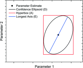

Fig. 2 Graphical representation of A-, D- and E-criteria to describe parameter estimate uncertainty.

• The A-criterion minimises the trace of the covariance matrix (sum of the elements in the main diagonal). This is proportional to the volume of the polyhedron circumscribing the confidence ellipsoid.

• The D-criterion minimises the determinant of the covariance matrix. This is proportional to the volume of the confidence ellipsoid.

• The E-criterion minimises the largest eigenvalue of the covariance matrix. This corresponds to minimising the length of the longest axis of the confidence ellipsoid.

While in parameter estimation problems the covariance matrix is calculated using the already collected experimental data, in MBDoE the expected covariance matrix after M_exp new experiments, V_θ,expected, can be calculated using the additivity of Fisher information according to eqn (9) where H_expected,i is the expected information from the i^th planned experiment and V_θ,0 is the preliminary covariance matrix from the N_exp already completed experiments. Note that in order to compute H_expected,i it is necessary to use the current parameter estimates [small straight theta, Greek, circumflex].

The MBDoE problem is an optimisation problem to find the values of the design vector φ, within a pre-defined allowable design space, which minimise a certain measure of the expected covariance matrix using one of the previously described methods of quantifying the size of a matrix² as shown in eqn (10).

φ = arg min ψ(V_θ,expected) (10)

The design vector φ, consists of all the control variables for the experiment.

Kinetic model

The reactor model in this work was the ideal plug flow reactor, shown in eqn (11) for transient conditions and in eqn (12) for steady-state conditionswhere C_BA is the concentration of benzoic acid (M), V is the reactor volume (L), v is volumetric flowrate (L min⁻¹) and r_BA (mol L⁻¹ min⁻¹) is the reaction rate of benzoic acid. Due to the large excess of ethanol used (molar ratio greater than 9 : 1) the reverse reaction was assumed to be negligible. Additionally, as the excess ethanol concentration can be considered constant, the ethanol dependence in the rate law was lumped with the pre-exponential factor, hence the rate laws were functions of temperature and benzoic acid only.⁶⁶ Thus, only two different irreversible kinetic rate laws were proposed, as shown in eqn (13a) and (b).

r_BA = −kC_BA (13a)

r_BA = −kC_BA² (13b)

To avoid any potential high correlation between the pre-exponential factor, k₀ (units are either min⁻¹ or L mol⁻¹ min⁻¹ depending on if the reaction is 1^st or 2^nd order), and activation energy, E_a (J mol⁻¹), the Arrhenius expression was written in the parameterised form shown in eqn (14), as this is shown to give the most accurate results and lead to fewer numerical problems during both parameter estimation and experiment design.⁶⁹

where T_M is the mean temperature 378.15 K, which was the average of the maximum and minimum temperature values, and KP1 (dimensionless) and KP2 (J mol⁻¹) are the kinetic parameters to be estimated. The Arrhenius pre-exponential factor, k₀, and activation energy, E_a can be calculated from the estimated parameters KP1 and KP2 according to eqn (15) and (16).

E_a = KP2 × 10 000 (16)

The reactor conversion X, was calculated according to

where C_BA,in is the known benzoic acid inlet concentration and C_BA,out is the HPLC measured outlet concentration of benzoic acid.

Experimental protocols

There were four types of experimental campaigns conducted; all were automatically controlled by LabVIEW, so they could be run without researcher supervision.

i. Steady-state factorial campaigns: a campaign of 8 steady-state experiments designed using the factorial method. This was repeated twice to allow estimation of experimental error.

ii. Steady-state MBDoE campaigns: a campaign of 8 steady-state experiments, where the first 2 experiments were pre-selected by the user and the following 6 experiments were designed by sequential MBDoE. This was repeated twice, once using the D-criterion and once with the E-criterion optimal design.

iii. Single-variable transient campaigns: a transient experiment where flowrate was ramped, while keeping all other variables constant. Due to the plug flow behaviour this was equivalent to an isothermal batch reactor. This was repeated at two different temperatures, where all experimental conditions (temperature, feed concentration, initial flowrate and ramp rate) were chosen by the user.

iv. Two-variable transient campaigns: a transient experiment where flowrate and temperature were simultaneously ramped. The experimental conditions (feed concentration, initial flowrate, initial temperature and ramp rates) were chosen by the user. This was done for two different sets of experimental conditions, one designed to explore a wide area of the design space, and the other designed by trial and error to minimise parameter uncertainty.

Steady-state factorial campaigns. In the first experimental campaign, the autonomous reactor platform ran a set of 8 steady-state experiments with conditions given in advance by the user. The list of experimental conditions was designed using a full factorial method of the three control variables at two levels (temperature 120 and 140 °C, flowrate 10 and 20 μL min⁻¹ and inlet benzoic acid concentration 1 and 1.5 M). The autonomous platform would run each experimental condition for 1 h to allow the reactor to reach steady-state before measuring the outlet concentration, performing online parameter estimation with a pre-selected kinetic model and moving to the next experimental condition. This campaign can then be viewed as the traditional benchmark against which the next methods (MBDoE and transient experiments) can be compared. In order to assess the experimental reproducibility, the full factorial campaign was repeated. The data collected from the factorial campaigns were used to identify the most suitable kinetic model, by using the previously described goodness of fit χ² test.

In these steady-state campaigns parameter estimation was performed online (using the 1^st order rate law in eqn (13a)) after each successive experiment starting from the second experiment (parameter estimation was not conducted after the first experiment, as a minimum of two different temperatures are needed before an activation energy can be estimated). The Nelder–Mead simplex algorithm was used for parameter estimation, and this required an initial guess for the parameter values. For the 1^st parameter estimation problem, conducted after 2 experiments, the initial guess for the parameter values were 8.97 and 7.6 based on some initial experimental data. For all the following parameter estimation problems (after experiments 3 to 8), the initial guess for the parameter values were the maximum likelihood estimate values obtained from the previous experiment.

Steady-state MBDoE campaigns. In these experimental campaigns, steady-state experiments were designed automatically by MBDoE. This required a model to be chosen by the user in advance of the experiments. The model chosen (based on the results from the factorial experimental campaigns, which will be discussed in the results section) was the steady-state ideal plug flow reactor model (eqn (12)) combined with the first order rate law (eqn (13a)). Parameter estimates are required to conduct MBDoE, however rather than providing the platform with an initial parameter guess and designing all experiments with MBDoE, it was decided instead to first run 2 experimental conditions chosen in advance by the user (140 °C, 20 μL min⁻¹, 1.5 M benzoic acid feed concentration and 120 °C, 10 μL min⁻¹, 1 M benzoic acid feed concentration). The experimental data collected from these 2 initial experiments enabled online parameter estimation, and these estimates were used for designing the next experiment with MBDoE. All subsequent experiments were designed with MBDoE using the updated parameter estimates from the previous experiment. In this way the MBDoE campaign was completed without requiring any estimate of the parameter value from the user. The ranges for the three control variables were 70–140 °C, 7.5–30 μL min⁻¹ and 0.9–1.55 M feed concentration. The upper temperature limit was chosen as 140 °C, because above this temperature the ethanol would evaporate at the system pressure of 6 barg. The lower flowrate limit was chosen in order to prevent excessively long reactor residence times and the upper concentration limit was chosen considering the maximum solubility of benzoic acid in ethanol. Each steady-state experiment was run for 65 min, and both D- and E-optimal MBDoE algorithms were used. The SLSQP (Sequential Least Squares Programming) algorithm was used for the MBDoE optimisation (see eqn (10)), and this required an initial guess for the optimum design (the optimum combination of temperature, flowrate and feed concentration). To mitigate the problem of incurring into local minima, an initial guess design vector was obtained by screening 10 000 randomly generated designs uniformly spread over the allowable design space. Each screening design was simulated and the predicted covariance matrix was calculated and quantified using either the D- or E-criterion. The screening design that produced the smallest covariance matrix was used as the initial design guess to initialise the SLSQP algorithm. This screening procedure was performed online every time the MBDoE algorithm was used, as the best screening design changed when the parameter estimates changed.

Single-variable transient campaigns. These experimental campaigns comprised of two transient experiments where the inlet flowrate to the reactor was ramped, while keeping the temperature constant. While other faster protocols of transient experiments exist, such as those which involve a step change of variables,⁴² these are not possible in this system due to the long analysis time required by the HPLC. The ramping approach used in this work can be adjusted for slow analysis methods by reducing the ramp rate, so a sufficient amount of data points can be collected before the ramp is completed. The ramped transient experiment was conducted twice, once at a temperature of 120 °C and an inlet benzoic acid concentration of 1.5 M and once at a temperature of 140 °C and an inlet benzoic acid concentration of 1.02 M. In both cases the initial flowrate was 100 μL min⁻¹ and the flowrate was reduced at a rate of 1 μL min⁻². In order to estimate the two parameter values, it was necessary to run two transient experiments at two different temperatures, and since each transient experiment took 100 min, both experiments were completed in under 4 h. For this experiment type we did not employ online parameter estimation, as two transient experiments conducted at two different temperatures are required to estimate the kinetic parameters. Instead the parameter estimation was conducted offline using the gPROMs ModelBuilder software (PSE). The data obtained from the transient experiments was analysed using the transient plug flow reactor model, as shown in eqn (11), along with the kinetic model shown in eqn (13a) and with an expression for the linear change in liquid flowrate as shown in eqn (18),

v = v₀ − α × t (18)

where v₀ is the initial flowrate (μL min⁻¹) and α is the rate at which the flowrate is decreasing (μL min⁻²). However, in this system the measurement was not taken exactly at the reactor exit, as there was a length of tubing connecting the reactor exit to the HPLC sample loop. This dead volume (44.2 μL) must be accounted for in order to relate the time at which a sample was measured, t_M, to the time it left the reactor, t_L.^22,29 This is shown in eqn (19),where V_dead is the dead volume (μL). A derivation of eqn (19) is included in the ESI.†

Two-variable transient campaigns. In these experimental campaigns, both the temperature and flowrate were ramped simultaneously to allow the exploration of a greater portion of the design space in a single experiment. The linear rate of change in temperature was modelled using eqn (20),

T = T₀ − β × t (20)

where T₀ is the initial temperature (K) and β is the rate of decrease in temperature (K min⁻¹). Here, only a single experiment requiring 100 min was necessary to conduct parameter estimation. Two experiments were conducted with different control variable profiles to demonstrate the effect of the experimental design. The first experiment design, called “wide spacing” was chosen based on commonly accepted rules of thumb, that exploring a wide region of the design space is beneficial for planning experiments. This design had an initial flowrate of 100 μL min⁻¹, which was ramped down at a rate of 1 μL min⁻² and the initial temperature was 140 °C, which was ramped down at a rate of 0.5 °C min⁻¹, the feed concentration was held constant at 1.50 M. The second experiment, called “improved design” was carefully designed by simulating many experiments and choosing the one which produced the smallest covariance matrix. The parameter estimates from the steady-state factorial campaign were used to simulate these experiments and the optimal design was found to have an initial flowrate of 30 μL min⁻¹, which was ramped down at a rate of 0.25 μL min⁻² and the initial temperature was 140 °C, which was ramped down at a rate of 0.2 °C min⁻¹, the feed concentration was held constant at 1.55 M.

Integration of Python scripts in LabVIEW

The autonomous platform was developed using a combination of LabVIEW (National Instruments) and Python, where LabVIEW was used to control lab equipment and monitor process values and Python was used to perform online parameter estimation, online MBDoE and also reading and writing the experimental results to Excel files. The integration of LabVIEW and Python was facilitated through the use of the LabVIEW-Python integration toolkit. The major advantage of using LabVIEW is that many commercial manufacturers of lab equipment make instrument drivers specifically for LabVIEW. Therefore, LabVIEW and its large collection of instrument drivers enable the easy and quick integration of multiple pieces of equipment. In this work, instrument drivers were available for the syringe pumps, heater, temperature and pressure sensors. However, there was no instrument driver available for the Jasco HPLC. For this reason the HPLC could not be directly integrated to the LabVIEW environment. Instead an alternative was developed, where the Jasco commercial software “ChromeNav” automatically triggered the HPLC measurement every 7 min and wrote the measured peak areas to an Excel file which could be accessed by the LabVIEW-Python code. A similar approach was reported in the literature for a GC system which also did not provide instrument drivers.¹⁴

One of the major issues of autonomous systems is that they are task-specific and that small changes in the experimental set-up require significant work to update the system. This can lead to situations where it is faster to conduct experiments manually than to develop automation algorithms for each new version of an experimental set-up.¹⁴ However, the LabVIEW code developed can be used with different equipment types, allowing this platform to be used for numerous reaction systems with only minor changes to the LabVIEW code. For example, without changing any LabVIEW code it is possible to replace the rope heater oil bath with a cartridge heater typically used to heat silicon-glass or glass microreactors. Additionally, with some simple changes to the LabVIEW code it is possible to incorporate different analysis methods, such as online Raman, UV or IR spectroscopy if such equipment were available.

For the steady-state experiments, the LabVIEW platform allowed the user to either implement a list of pre-selected experimental conditions, or to run a campaign of steady-state experiments, which were designed online by MBDoE algorithms written and executed in Python. In both cases the LabVIEW code ran an experimental condition for a duration of time specified by the user to ensure the reactor reached steady-state. When the specified time limit was reached, the LabVIEW code read the most recent HPLC measurement and took this value as the steady-state outlet concentration for that experimental condition. These experimental conditions and outlet concentrations were then written in a “Record” Excel file with all the previous experimental results. LabVIEW then called a Python function (involving the Nelder–Mead simplex algorithm) to perform parameter estimation using the “Record” Excel file as the Python function input. The computed parameter statistics were then displayed on the LabVIEW screen and were also written to the “Record” Excel file. The LabVIEW code measured and recorded the temperatures, flowrates and pressures every 5 s and saved the values in a separate “Process Value” Excel file, allowing the user to examine the experimental conditions at some later date. Additionally, the LabVIEW code had safety shutdown features, where if any temperature or pressure exceeded a user specified value the pumps and heater were automatically turned off. A detailed description of the LabVIEW code is provided in the ESI.†

Results and discussion

Steady-state factorial campaigns – model discrimination

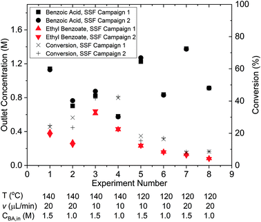
The results of the two identical steady-state factorial campaigns (see Fig. 3), showed that the system behaved well with high reproducibility. Values of the steady-state outlet concentrations for each experimental condition are reported in the ESI† and it is shown that the average mole balance closed to within 95%. In order to identify the appropriate rate law from the two candidate models described in eqn (13a) and (13b), the χ² test was applied to the data obtained from the factorial campaigns for both models. The results of the χ² test are shown in Table 1, where it is observed that model 13b, which had 2^nd order kinetics with respect to benzoic acid, must be rejected. As only a single candidate model remained after the initial factorial screening, it was not necessary to conduct further experiments designed by MBDoE algorithms for model discrimination.⁵³ The estimated parameter values of KP1 and KP2 obtained from a single campaign of 8 experiments designed by the steady-state factorial campaigns were 9.11 and 7.98. These estimates correspond to a pre-exponential of 11.65 × 10⁶ s⁻¹ and activation energy of 79.8 kJ mol⁻¹. In the literature the only work that employed similar experimental conditions selected a kinetic model which was 2^nd order with respect to benzoic acid. However, the activation energy of 80.5 kJ mol⁻¹ reported⁶⁶ is in agreement with our results.

Fig. 3 Outlet concentrations of benzoic acid and ethyl benzoate and benzoic acid conversion for the two identical steady-state factorial (SSF) campaigns, each consisting of 8 steady-state experiments.

Table 1 Data fitting results for two candidate kinetic models using experimental data from the two identical steady-state factorial campaigns

Eqn	Model	χ ^2 (χref^2 = 43.7)	Result
13a	r = kCBA	16.2	Possible model
13b	r = kCBA^2	156	Reject model

---

Steady-state MBDoE campaigns – parameter precision

The experimental conditions designed by the two steady-state MBDoE campaigns, D- and E-optimal, are shown in Fig. 4 (with the outlet concentrations shown in the ESI†). After the initial 2 experiments chosen by the user to be the opposite corners of the previously used factorial design space, the autonomous platform executed MBDoE algorithms to design each experiment sequentially, using the information gathered from previous experiments. It is observed that the MBDoE algorithms always designed experiments with the maximum feed concentration of benzoic acid (1.55 M) and minimum flowrate (7.5 μL min⁻¹). This is because the maximum feed concentration and minimum flowrate minimised the expected covariance matrix, which also meant that these experiments carried the greatest level of Fisher information. The optimal temperature for experiments was found to alternate between the maximum temperature allowed (140 °C) and lower temperatures in the range 110 °C–120 °C). For the D-optimal campaign the MBDoE algorithm chose to run the same experimental conditions (140 °C, 7.5 μL min⁻¹, 1.55 M) three times, whereas the E-optimal campaign only designed 1 experiment at this condition and placed the other 5 designed experiments in the low temperature region. The occurrence of repeated experiments designed by MBDoE methods is well documented in the literature, because repeated experiments in a highly informative region are more useful for parameter precision than a number of different experiments spread across a wide but lowly informative design space, so experiment replication is not surprising.^69,70 The E-optimal campaign explored lower temperatures than the D-optimal, possibly because the wider temperature range explored helped to reduce correlation between the two parameters.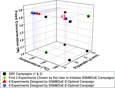

Fig. 4 Experimental conditions utilised by the steady-state factorial (SSF) and steady-state MBDoE (SSMBDoE) campaigns.

The parameter estimates and the associated statistics (including t-values, confidence intervals and χ² tests) from the steady-state factorial and the steady-state MBDoE experiments are compared in Table 2. The parameter estimates are similar for all campaigns, however the 95% confidence intervals are substantially smaller and the t-values substantially larger for the MBDoE campaigns. This demonstrates the benefits of online MBDoE for identifying kinetic models. As there are only two parameters in this model it is also possible to show these results graphically in the form of confidence ellipsoids in Fig. 5, where we can observe that both the steady-state MBDoE campaigns produce confidence ellipsoids which are much smaller than the steady-state factorial campaigns. Similarly, it is observed that the E-optimal campaign produces a shorter (but “fatter”) confidence ellipsoid than the D-optimal campaign, as the E-optimal campaign aims to minimise the length of the longest axis of the confidence ellipsoid. Additionally, Fig. 6 shows the diminishing return on conducting multiple experiments. For both the steady-state factorial and the steady-state MBDoE campaigns, after conducting 5 experiments the determinant of the covariance matrix (directly proportional to the volume of the confidence ellipsoid) did not get much smaller with further experiments in the allowable design space.

Table 2 Parameter estimates and statistics obtained from the steady-state factorial (SSF) and the steady-state MBDoE (SSMBDoE) campaigns. KP1 and KP2 are reparametrized forms of the Arrhenius parameters, as shown in eqn (14)–(16)

Campaign	KP1 ± 95% confidence interval	KP2 ± 95% confidence interval	KP1 95% t-value	KP2 95% t-value	t ref	χ ^2	χ ^2 ref	k 0 (s^−1)	E a (kJ mol^−1)
SSF 1	9.06 ± 0.19	7.84 ± 0.75	48.0	10.5	1.76	14.9	23.7	7.85 × 10^6	78.4
SSF 2	9.11 ± 0.19	7.98 ± 0.77	46.9	10.4	1.76	0.98	23.7	11.7 × 10^6	79.8
SSMBDoE D-optimal	9.17 ± 0.12	8.15 ± 0.46	79.1	17.6	1.76	10.6	23.7	18.8 × 10^6	81.5
SSMBDoE E-optimal	9.17 ± 0.10	8.12 ± 0.43	95.5	18.8	1.76	6.11	23.7	17.1 × 10^6	81.2

---

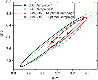Fig. 5 Statistical certainty of the parameters KP1 and KP2 for the steady-state factorial (SSF) and steady-state MBDoE (SSMBDoE) D- and E-optimal campaigns, as illustrated by the 95% confidence ellipsoids. KP1 and KP2 are reparametrized forms of the Arrhenius parameters, as shown in eqn (14)–(16).

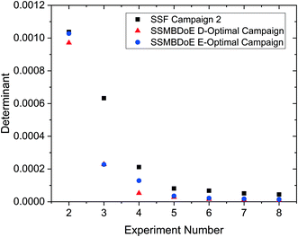Fig. 6 Determinant of the covariance matrix against number of experiments conducted for the steady-state factorial (SSF) and the steady-state MBDoE (SSMBDoE) D- and E-optimal campaigns.

Single-variable transient campaigns

The outlet concentrations of the transient experiments, where only flowrate was ramped while keeping temperature constant are shown in Fig. 7, while numerical values are shown in the ESI.† The parameter values estimated from the data gathered in these experiments, along with the statistical tests including χ², t-values and confidence intervals are shown in Table 3. The parameter estimates from the transient experiments are consistent with the estimates from the steady-state factorial campaign. Additionally, the parameter precision, as measured by the 95% confidence intervals is approximately equal for the transient and steady-state factorial experiments, despite the fact that the two transient experiments took only 4 h to perform instead of the 8 h required for the steady-state campaign. The transient experiments also required less reactant, hence this method offers considerable scope for saving both time and cost in the case of systems with expensive reactants. It should be noted that the experiments in the steady-state factorial campaigns were not optimised for maximum time efficiency. The steady-state experimental duration of 1 h was chosen to be the most efficient for the slower experiments in the campaign, those that used a 10 μL min⁻¹ flowrate. The 20 μL min⁻¹ flowrate steady-state experiments, which had shorter residence times could finish in just 40 min. Thus, if the experiment duration was linked to the experiment residence time, it is possible that the steady-state factorial campaign could have been completed in 6.7 h.

Fig. 7 Control variable profile and outlet concentrations of benzoic acid (BA) and ethyl benzoate (EB) obtained by automated HPLC measurements from the single-variable transient campaigns, where flowrate was isothermally ramped at a) 120 °C and b) at 140 °C.

Table 3 Parameter estimates and statistics obtained from the single-variable transient (SVT) campaign compared to the steady-state factorial (SSF) campaign 2. KP1 and KP2 are reparametrized forms of the Arrhenius parameters, as shown in eqn (14)–(16)

Campaign	KP1 ± 95% confidence interval	KP2 ± 95% confidence interval	KP1 95% t-value	KP2 95% t-value	t ref	χ ^2	χ ref ^2	k 0 (s^−1)	E a (kJ mol^−1)
SVT	9.03 ± 0.18	7.63 ± 0.76	49.1	10.0	1.68	25.9	67.5	4.15 × 10^6	76.3
SSF 2	9.11 ± 0.19	7.98 ± 0.77	46.9	10.4	1.76	0.98	23.7	11.7 × 10^6	79.8

---

Two-variable transient campaigns

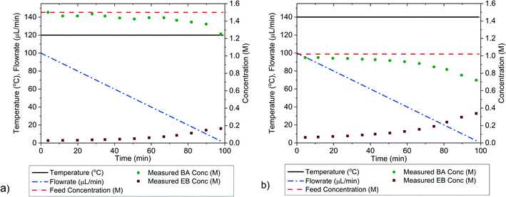
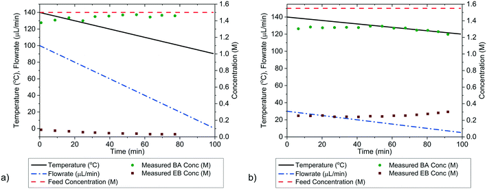
It is possible to further minimise the time required to gather enough kinetic data to allow for parameter estimation by ramping both temperature and flowrate simultaneously in a transient experiment. Such an experiment requires less than 2 h to complete, but still explores a large area of the design space. For this transient experiment it is necessary for the user to select the initial values of temperature, flowrate and concentration, as well as appropriate ramp rates for both temperature and flowrate. It was found that the choice of these variables was not intuitive and that a poor selection of values would lead to parameter estimates of low precision. This was demonstrated for the first experiment, called “wide spacing”, where the initial flowrate was 100 μL min⁻¹ and ramped down at 1 μL min⁻², while the temperature was simultaneously ramped down from an initial temperature of 140 °C at a rate of 0.5 °C min⁻¹, with constant feed concentration of 1.5 M, as shown in Fig. 8a. These control variable profiles were chosen as they covered a wide section of the design space, spanning from 140 to 90 °C and from 100 to 1 μL min⁻¹, so it was expected that they would lead to precise parameter estimation. However, it was later shown that this “wide spacing” experiment design was poor, leading to large 95% confidence ellipsoids, as shown in Fig. 9, and large confidence intervals, as shown in Table 4. The cause of the low parameter precision can be attributed to the experiment being conducted in a low information region of the design space. Looking at the measured outlet concentrations from the experiment in Fig. 8a, we speculate that the experiment design is poor due to the low conversions attained, which were always less than 6%. Therefore, it was difficult to estimate the kinetic parameters, as the reaction was never allowed to progress to significant levels and because the concentration change between the feed and the outlet value (typically less than 0.1 M) was only slightly larger than the measurement error (0.030 M for benzoic acid and 0.0165 M for ethyl benzoate).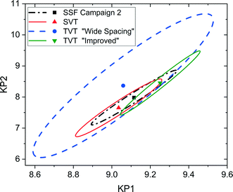

Fig. 8 Control variable profiles and outlet concentrations of benzoic acid (BA) and ethyl benzoate (EB) obtained by automated HPLC measurements for the two-variable transient campaigns, where flowrate and temperature were ramped simultaneously. Figure a) is the “wide spacing” design chosen by the user to cover a wide range of experimental conditions, and figure b) is the “improved” design chosen from screening many designs in simulated experiments.

Fig. 9 Statistical certainty of the parameters KP1 and KP2 for the steady-state factorial (SSF), single-variable transient (SVT) and two-variable transient (TVT) “wide spacing” and “improved” campaigns, as illustrated by the 95% confidence ellipsoids. KP1 and KP2 are reparametrized forms of the Arrhenius parameters, as shown in eqn (14)–(16).

Table 4 Parameter estimates and statistics obtained from the two-variable transient (TVT) campaigns, “wide spacing” and “improved”, where flowrate and temperature were ramped simultaneously, compared to the steady-state factorial (SSF) campaign 2

Campaign	KP1 ± 95% confidence interval	KP2 ± 95% confidence interval	KP1 95% t-value	KP2 95% t-value	t ref	χ ^2	χref^2	k 0 (s^−1)	E a (kJ mol^−1)
TVT “wide spacing”	9.06 ± 0.4	8.36 ± 1.97	22.7	4.24	1.72	4.77	31.4	41.0 × 10^6	83.6
TVT “improved”	9.25 ± 0.17	8.45 ± 0.86	52.9	9.73	1.70	4.15	38.9	45.2 × 10^6	84.5
SSF 2	9.11 ± 0.19	7.98 ± 0.77	46.9	10.4	1.76	0.98	23.7	11.7 × 10^6	79.8

---

In order to identify more suitable operating conditions, the parameter estimates from the steady-state factorial experiments were used to run simulated transient experiments, which were then used for parameter estimation. By simulating many different transient experiments with different control variable profiles and then examining the resulting parameter estimate statistics, it was possible to identify good and bad experiment designs. By trial and error the best simulated experimental design was found to be an initial flowrate of 30 μL min⁻¹, which was ramped down at a rate of 0.25 μL min⁻², along with a temperature profile that started at 140 °C and was ramped down at a rate of 0.2 °C min⁻¹, the feed concentration was held constant at 1.55 M. This best design was then run on the autonomous system. The control variable profiles and the resulting measured outlet concentrations are shown in Fig. 8b, where it can be observed that much higher conversions of up to 20% were achieved. The kinetic data obtained from this second “improved” design experiment led to much more precise parameter estimates, as shown by the narrower confidence intervals in Table 4 and the smaller 95% confidence ellipsoid in Fig. 9. The 95% confidence ellipsoid was much smaller than the previous “wide spacing” experiment, and was also only slightly larger than the confidence ellipsoid from the campaign of factorial experiments, despite the fact that the transient experiment required only 2 h compared to 8 h for the factorial campaign. When making comparisons between experimental methods used in this work, it is important to note that the two-variable transient “improved” design was the only campaign that used prior information (as it used parameter estimates from the steady-state factorial campaign for the simulations to find the improved design). Therefore, comparison between the two-variable transient “improved” campaigns with others must be done with caution, as no other campaign required such prior information. However, such an experimental strategy could be used if initial parameter estimates were available from the literature. For more complex systems where no initial parameter values can be estimated from the literature, this work demonstrates the difficulties in designing transient experiments without parameter estimates, as the precision obtained varies greatly depending on the design. In such situations, it may be advisable to begin with easily designed steady-state experiments, to generate the data required for parameter estimation, before designing transient experiments. Overall, the comparison between the steady-state and transient experiments in Fig. 9 demonstrates a trade-off between time and parameter precision, where the most precise parameter estimates were obtained from a campaign of steady-state experiments, while the transient experiments offered the fastest way of generating kinetic data, but with progressively lower precision.

Conclusion

In this work an autonomous microreactor platform for the rapid identification of reaction kinetics has been developed. This platform combines the advantages of flow microreactors, online analysis and automation to create a lab tool that can save researchers time and resources. Using the case study of esterification of benzoic acid and ethanol with homogenous sulfuric acid catalyst, the platform was tested in 4 experimental campaigns; i) automatically conducting 2 campaigns of 8 steady-state experiments designed by full factorial, ii) conducting 2 campaigns of steady-state experiments designed by D- and E-optimal MBDoE, iii) conducting 2 transient campaigns where flowrate was ramped to simulate an isothermal batch reactor at 2 different temperatures and iv) conducting 2 transient campaigns where flowrate and temperature were both ramped simultaneously, once designed to achieve wide exploration of the design space and once where the best design was obtained from simulated experiments. All experimental campaigns were in general agreement, giving similar parameter estimates as demonstrated by the overlapping confidence ellipsoids. When comparing the various experimental campaigns it is clear that transient experiments offered the fastest way to identify kinetic parameters, while also using the least amount of reagents. When flowrate and temperature were ramped simultaneously parameter estimates could be obtained in less than 2 h, however the precision of these estimates varied dramatically with the transient control variable profiles chosen by the user, which are difficult to choose unless there is already some prior information about the kinetic parameters. The slightly slower method of isothermally ramping flowrate, which required two transient experiments at two different temperatures, gave more precise parameter estimates in only 4 h. The most precise parameter estimates were obtained from the steady-state MBDoE experiments, where the 8 experiments showed significantly smaller confidence ellipsoids than those obtained from the same number of steady-state experiments designed by the factorial method. It is important to note that while MBDoE provides substantial benefits compared to a factorial campaign for developing a model with highly precise parameter estimates, this comes at the cost of reduced exploration of the design space making it harder to test the domain of validity of the model. Therefore MBDoE for parameter precision should only be used when there is already high confidence in the validity of the model, which can be achieved by conducting a widely spaced factorial campaign, and if necessary this can be followed by a campaign of experiments designed by MBDoE for model discrimination.

An important factor when selecting what type of experiments to conduct (transient or steady-state) is the relevant time scales for the reactor to reach a new steady-state compared to the analysis method. In cases where the analysis time is significantly less than the time required for the reactor to reach steady-state, there is an advantage in using transient experiments for saving time and reagents. If the analysis method is fast, or the reactor residence time is long, conducting transient experiments would be preferable to running steady-state campaigns. In contrast, if the analysis method is long compared to the reactor residence time, then a campaign of steady-state experiments may be preferable, initially designed by factorial methods to allow model discrimination and validation before a second MBDoE campaign is performed to target parameter estimation.

Conflicts of interest

There are no conflicts of interest to declare.

Acknowledgements

The authors CW and AP thank the department of Chemical Engineering, University College London, for their funding. MQ thanks the Hugh Walter Stern PhD Scholarship, University College London for funding. All the authors express their gratitude to Dr Gaowei Wu who designed the custom-made PEEK pressure vessel used in this work.

References

1. G. Franceschini and S. Macchietto, Ind. Eng. Chem. Res., 2008, 47, 2331–2348.
2. G. Franceschini and S. Macchietto, Chem. Eng. Sci., 2008, 63, 4846–4872.
3. M. W. Losey, M. A. Schmidt and K. F. Jensen, Ind. Eng. Chem. Res., 2001, 40, 2555–2562.
4. C. Yang, A. R. Teixeira, Y. Shi, S. C. Born, H. Lin, Y. Li Song, B. Martin, B. Schenkel, M. Peer Lachegurabi and K. F. Jensen, Green Chem., 2018, 20, 886–893.
5. N. Al-Rifai, E. Cao, V. Dua and A. Gavriilidis, Curr. Opin. Chem. Eng., 2013, 2, 338–345.
6. B. Gutmann, D. Cantillo and C. O. Kappe, Angew. Chem., Int. Ed., 2015, 54, 6688–6728.
7. J. Yoshida, A. Nagaki and T. Yamada, Chem. – Eur. J., 2008, 14, 7450–7459.
8. T. Salmi, J. Hernández Carucci, M. Roche, K. Eränen, J. Wärnå and D. Murzin, Chem. Eng. Sci., 2013, 87, 306–314.
9. J. Zhang, Y. Lu, Q. Jin, K. Wang and G. Luo, Chem. Eng. J., 2012, 203, 142–147.
10. S. Tadepalli, R. Halder and A. Lawal, Chem. Eng. Sci., 2007, 62, 2663–2678.
11. B. Walsh, J. R. Hyde, P. Licence and M. Poliakoff, Green Chem., 2005, 7, 456–463.
12. A. J. Parrott, R. A. Bourne, G. R. Akien, D. J. Irvine and M. Poliakoff, Angew. Chem., Int. Ed., 2011, 50, 3788–3792.
13. A. Echtermeyer, Y. Amar, J. Zakrzewski and A. Lapkin, Beilstein J. Org. Chem., 2017, 13, 150.
14. N. Cherkasov, Y. Bai, A. J. Expósito and E. V. Rebrov, React. Chem. Eng., 2018, 3, 769–780.
15. K. Koch, B. J. A. van Weerdenburg, J. M. M. Verkade, P. J. Nieuwland, F. P. J. T. Rutjes and J. C. M. van Hest, Org. Process Res. Dev., 2009, 13, 1003–1006.
16. T. C. Malig, J. D. B. Koenig, H. Situ, N. K. Chehal, P. G. Hultin and J. E. Hein, React. Chem. Eng., 2017, 2, 309–314.
17. J. P. McMullen and K. F. Jensen, Org. Process Res. Dev., 2010, 14, 1169–1176.
18. B. J. Reizman, Y.-M. Wang, S. L. Buchwald and K. F. Jensen, React. Chem. Eng., 2016, 1, 658–666.
19. J. P. McMullen and K. F. Jensen, Org. Process Res. Dev., 2011, 15, 398–407.
20. D. C. Patel, Y. F. Lyu, J. Gandarilla and S. Doherty, Anal. Chim. Acta, 2018, 1004, 32–39.
21. N. Holmes, G. R. Akien, A. J. Blacker, R. L. Woodward, R. E. Meadows and R. A. Bourne, React. Chem. Eng., 2016, 1, 366–371.
22. C. A. Hone, N. Holmes, G. R. Akien, R. A. Bourne and F. L. Muller, React. Chem. Eng., 2017, 2, 103–108.
23. A.-C. Bédard, A. Adamo, K. C. Aroh, M. G. Russell, A. A. Bedermann, J. Torosian, B. Yue, K. F. Jensen and T. F. Jamison, Science, 2018, 361, 1220–1225.
24. D. E. Fitzpatrick, C. Battilocchio and S. V. Ley, Org. Process Res. Dev., 2015, 20, 386–394.
25. N. Holmes, G. R. Akien, R. J. D. Savage, C. Stanetty, I. R. Baxendale, A. J. Blacker, B. A. Taylor, R. L. Woodward, R. E. Meadows and R. A. Bourne, React. Chem. Eng., 2016, 1, 96–100.
26. D. Perera, J. W. Tucker, S. Brahmbhatt, C. J. Helal, A. Chong, W. Farrell, P. Richardson and N. W. Sach, Science, 2018, 359, 429–434.
27. K. L. A. Chan, X. Niu, A. J. de Mello and S. G. Kazarian, Lab Chip, 2010, 10, 2170.
28. E. Gross, X.-Z. Shu, S. Alayoglu, H. A. Bechtel, M. C. Martin, F. D. Toste and G. A. Somorjai, J. Am. Chem. Soc., 2014, 136, 3624.
29. J. S. Moore and K. F. Jensen, Angew. Chem., Int. Ed., 2014, 53, 470–473.
30. J. S. Moore and K. F. Jensen, Org. Process Res. Dev., 2012, 16, 1409–1415.
31. K. C. Aroh and K. F. Jensen, React. Chem. Eng., 2018, 3, 94–101.
32. R. A. Skilton, A. J. Parrott, M. W. George, M. Poliakoff and R. A. Bourne, Appl. Spectrosc., 2013, 67, 1127–1131.
33. M. F. Roberto, T. I. Dearing, S. Martin and B. J. Marquardt, J. Pharm. Innov., 2012, 7, 69–75.
34. E. Cao, G. Brett, P. J. Miedziak, J. M. Douthwaite, S. Barrass, P. F. McMillan, G. J. Hutchings and A. Gavriilidis, Catal. Today, 2017, 283, 195–201.
35. V. Sans, L. Porwol, V. Dragone and L. Cronin, Chem. Sci., 2015, 6, 1258–1264.
36. A. M. Alb, M. F. Drenski and W. F. Reed, Polym. Int., 2008, 57, 390–396.
37. J. R. Goodell, J. P. McMullen, N. Zaborenko, J. R. Maloney, C.-X. Ho, K. F. Jensen, J. A. Porco Jr and A. B. Beeler, J. Org. Chem., 2009, 74, 6169–6180.
38. B. J. Reizman and K. F. Jensen, Chem. Commun., 2015, 51, 13290–13293.
39. R. J. Berger, F. Kapteijn, J. A. Moulijn, G. B. Marin, J. De Wilde, M. Olea, D. Chen, A. Holmen, L. Lietti, E. Tronconi and Y. Schuurman, Appl. Catal., A, 2008, 342, 3–28.
40. S. D. Schaber, S. C. Born, K. F. Jensen and P. I. Barton, Org. Process Res. Dev., 2014, 18, 1461–1467.
41. K. Morgan, N. Maguire, R. Fushimi, J. Gleaves, A. Goguet, M. Harold, E. Kondratenko, U. Menon, Y. Schuurman and G. Yablonsky, Catal. Sci. Technol., 2017, 7, 2416–2439.
42. S. Mozharov, A. Nordon, D. Littlejohn, C. Wiles, P. Watts, P. Dallin and J. M. Girkin, J. Am. Chem. Soc., 2011, 133, 3601–3608.
43. C. Houben and A. A. Lapkin, Curr. Opin. Chem. Eng., 2015, 9, 1–7.
44. S. V. Ley, D. E. Fitzpatrick, R. J. Ingham and R. M. Myers, Angew. Chem., Int. Ed., 2015, 54, 3449–3464.
45. V. Sans and L. Cronin, Chem. Soc. Rev., 2016, 45, 2032–2043.
46. J. P. McMullen, M. T. Stone, S. L. Buchwald and K. F. Jensen, Angew. Chem., Int. Ed., 2010, 49, 7076–7080.
47. R. A. Vieira, C. Sayer, E. L. Lima and J. C. Pinto, Ind. Eng. Chem. Res., 2002, 41, 2915–2930.
48. D. N. Jumbam, R. A. Skilton, A. J. Parrott, R. A. Bourne and M. Poliakoff, J. Flow Chem., 2012, 2, 24–27.
49. D. Cortés-Borda, K. V. Kutonova, C. Jamet, M. E. Trusova, F. O. Zammattio, C. Truchet, M. Rodriguez-Zubiri and F. O.-X. Felpin, Org. Process Res. Dev., 2016, 20, 1979–1987.
50. C. Houben, N. Peremezhney, A. Zubov, J. Kosek and A. A. Lapkin, Org. Process Res. Dev., 2015, 19, 1049–1053.
51. A. M. Schweidtmann, A. D. Clayton, N. Holmes, E. Bradford, R. A. Bourne and A. A. Lapkin, Chem. Eng. J., 2018, 352, 277–282.
52. G. E. Box and W. J. Hill, Technometrics, 1967, 9, 57–71.
53. G. B. Ferraris, P. Forzatti, G. Emig and H. Hofmann, Chem. Eng. Sci., 1984, 39, 81–85.
54. G. E. Box and H. Lucas, Biometrika, 1959, 46, 77–90.
55. N. R. Draper and W. G. Hunter, Biometrika, 1966, 53, 525–533.
56. D. C. Fabry, E. Sugiono and M. Rueping, Isr. J. Chem., 2014, 54, 341–350.
57. B. J. Reizman and K. F. Jensen, Acc. Chem. Res., 2016, 49, 1786–1796.
58. F. Galvanin, M. Barolo and F. Bezzo, Ind. Eng. Chem. Res., 2009, 48, 4415–4427.
59. F. Galvanin, S. Macchietto and F. Bezzo, Ind. Eng. Chem. Res., 2007, 46, 871–882.
60. F. Galvanin, E. Cao, N. Al-Rifai, A. Gavriilidis and V. Dua, Comput. Chem. Eng., 2016, 95, 202–215.
61. T. Lohmann, H. G. Bock and J. P. Schloeder, Ind. Eng. Chem. Res., 1992, 31, 54–57.
62. M. Fujiwara, Z. K. Nagy, J. W. Chew and R. D. Braatz, J. Process Control, 2005, 15, 493–504.
63. S. Issanchou, P. Cognet and M. Cabassud, AIChE J., 2005, 51, 1773–1781.
64. M. Cruz Bournazou, T. Barz, D. Nickel, D. Lopez Cárdenas, F. Glauche, A. Knepper and P. Neubauer, Biotechnol. Bioeng., 2017, 114, 610–619.
65. B. J. Reizman and K. F. Jensen, Org. Process Res. Dev., 2012, 16, 1770–1782.
66. G. Pipus, I. Plazl and T. Koloini, Chem. Eng. J., 2000, 76, 239–245.
67. O. Levenspiel, Chemical Reaction Engineering, Wiley, New York, 3rd edn, 1999.
68. Y. Bard, Nonlinear Parameter Estimation, Academic Press, New York, 1974.
69. G. Buzzi-Ferraris and F. Manenti, Chem. Eng. Sci., 2009, 64, 1061–1074.
70. M. Box, Journal of the Royal Statistical Society. Series B (Methodological), 1968, 30(2), 290–302.

---

Footnote

† Electronic supplementary information (ESI) available. See DOI: 10.1039/c8re00345a

---