DOI:
10.1039/D1RA03715C
(Paper)
RSC Adv., 2021,
11, 25764-25776
A property-oriented adaptive design framework for rapid discovery of energetic molecules based on small-scale labeled datasets†
Received
12th May 2021
, Accepted 8th July 2021
First published on 27th July 2021
Abstract
It remains an important challenge to apply machine learning in material discovery with limited-scale datasets available, in particular for the energetic materials. Motivated by the challenge, we developed a Property-oriented Adaptive Design Framework (PADF) to quickly design new energetic compounds with desired properties. The PADF consists of a search space, machine learning model, optimization algorithm and an evaluator based on quantum mechanical calculations. The effectiveness and generality of the PADF were assessed by two case studies on the heat of formation and heat of explosion as the target properties. 88 compounds were selected as the initial training dataset from the search space containing 84![[thin space (1/6-em)]](https://www.rsc.org/images/entities/char_2009.gif) 083 compounds generated. SVR.lin/Trade-off coupled with E-state + SOB and KRR/KG coupled with CDS + E-state + SOB were determined to be the best combination pairs for the heat of formation and the heat of explosion, respectively. Most of the ten compounds selected from the first ten iterations exhibit better properties than the optimal sample in the initial dataset. Besides, the heat of explosion as the target property outperforms the heat of formation in designing energetic compounds with high detonation performance. In particular, a new compound selected at the 3rd iteration exhibits high potential as an explosive. Our strategy could be extended to other domains limited by small-scale datasets labeled.
083 compounds generated. SVR.lin/Trade-off coupled with E-state + SOB and KRR/KG coupled with CDS + E-state + SOB were determined to be the best combination pairs for the heat of formation and the heat of explosion, respectively. Most of the ten compounds selected from the first ten iterations exhibit better properties than the optimal sample in the initial dataset. Besides, the heat of explosion as the target property outperforms the heat of formation in designing energetic compounds with high detonation performance. In particular, a new compound selected at the 3rd iteration exhibits high potential as an explosive. Our strategy could be extended to other domains limited by small-scale datasets labeled.
1 Introduction
The discovery of novel materials with desired properties can bring tremendous improvement in science and technology. However, the material exploration has historically been driven by the trial-and-error process, imposing high requirements for both resources and equipment. With rapid advances in computing power and mathematical algorithms, artificial intelligence (AI) has become a powerful tool in guiding experimental research studies.1 As an important subfield of AI, machine learning (ML) techniques could capture important information and map relationships underlying complicated data so that they show fascinating promise in diverse fields such as computer vision, medicine and chemistry.2,3 In material fields, ML techniques are also utilized to probe relationships between structures/compositions and properties.4,5 It is known that ML is a data-driven method, and the number of training data is a crucial factor for the robustness of the constructed inference model. However, compared with medicine and computer vision, labeled datasets in the material field are generally limited, in particular for energetic materials due to harsh and hazardous experimental conditions.6
As is known, the energetic materials have played a vital role in the military and civilian fields.7–9 With ever-growing needs for industry and military, research on the energetic materials has entered from the traditional compound stage into a new stage of high energy density materials (HEDMs). HEDMs composed of nitrogen-rich skeletons and energetic substituents exhibit promising potential for explosives.10 However, purely experimental investigations possess long cycle, high costs and risk, thus limiting the development of HEDMs. In order to assist experiments, quantum mechanics (QM) methods have been applied to obtain structural and energy-related properties as well as reaction mechanisms over decades.11–13 In spite of high accuracy of the QM calculations, it is computationally expensive to explore the enormous space of unknown energetic compounds. Thus, some ML-based works were utilized to quickly predict some properties of energetic materials, such as decomposition temperature,14 melting point,15 autoignition temperature,16 sensitivity and density.17,18 However, as mentioned above, the labeled data of the energetic compounds are very limited. Consequently, the applications of ML in the energetic materials generally suffer from prediction uncertainties when extrapolated to unknown chemical space. In addition, most of the previous ML-related works focused on the property prediction based on the structure, lacking the property-oriented structure design with higher efficiency. Recently, the Few-Shot Learning (FSL) paradigm was proposed to enable ML models to generalize with small-scale samples from the aspects of data, model and algorithm.19 Active learning is a typical framework of FSL, which utilizes an adaptive design strategy to help relieve the burden of obtaining large-scale data by means of machine learning prediction results coupled with an optimization algorithm, which can recommend the high-performing compound for the next test. Practically, the active learning paradigm has been successfully applied to some material fields like high entropy alloys, energy storage materials and piezoelectrics, which were validated by experimental synthesis.20–22
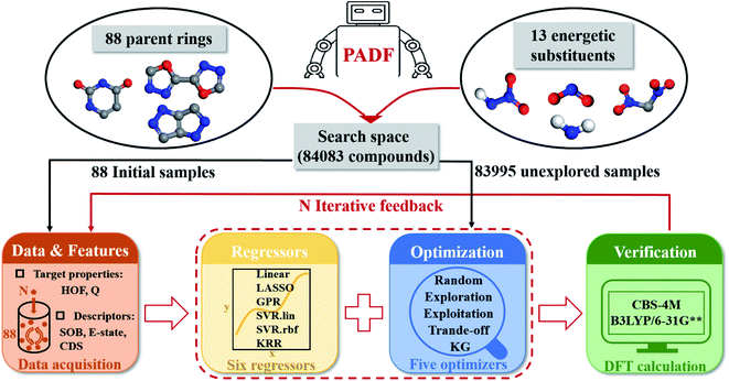
Motivated by the issue, we, in this work, developed a property-oriented adaptive design framework based on a small amount of datasets labeled, which can rapidly screen potential energetic compounds with desired properties from a vast chemical space unexplored. We name it Property-oriented Adaptive Design Framework (PADF). The PADF consists of a search space, a ML-based regression model (also called a regressor), an optimization function (also called an optimizer) and an evaluation system based on quantum mechanical calculations. Specifically, the search space unlabeled is generated by combining energetic parent rings and energetic substituents. The ML-based regression model is constructed based on a small-amount of labeled datasets to predict the unexplored samples in the search space. Combining the predictive value from the ML model and the uncertainty derived from the optimization function, a highly informative sample is screened from the unknown space and added into the training set to decrease uncertainty in the ML-based regression. Finally, the QM-based calculation is applied to validate the energetic properties. After iterative cycles, an efficient self-adaptive design framework could be constructed, through which the predictive ability of the ML model could be improved and the high-performing candidate could be quickly searched from the huge unknown space. Herein, we mainly focus on the two important energetic properties: heat of formation (HOF) and heat of explosion (Q). In fact, HOF often serves as a general target in the material domains, which is closely associated with the stability and the energy of materials, like perovskite solar cells,23 ionic liquids,24 and especially energetic materials.25 The heat of explosion is a specific and important property for the explosives. We first construct the PADF for the heat of formation. Then, we extend the PADF to the heat of explosion in order to further assess its performance on one side. On the other hand, we also hope to evaluate which property as the desired target is more beneficial to search the explosive with high performance.
2 Computational details
Our proposed PADF is constructed according to the flow chart in Fig. 1. The search space unexplored is generated by combining 88 parent rings and 13 energetic substituents, from which a small-scale initial dataset is selected to be labeled in order to train the ML-based regressor. In each iteration, a candidate compound will be selected from the search space in terms of the combination pair of the regressor and the optimizer. Then it is added into the initial training set after verifying its property by QM calculations. Accordingly, a feedback loop can be constructed to iteratively recommend candidates and improve the predictive capacity of the regressor.
 |
| | Fig. 1 The flowchart of the Property-oriented Adaptive Design Framework (PADF), which consists of a search space, a ML-based regressor, an optimizer, and an evaluation system based on quantum mechanical calculations. | |
2.1 Search space
The implementation of the PADF begins with a search space containing vast potential energetic compounds unexplored. Due to the lack of an existing energetic dataset, we constructed it by combining the 88 parent rings and the 13 energetic substituents collected from the literature involving energetic materials. Tables S1 and S2† show the chemical structures of the 88 parent rings and the 13 substituents. Substitution sites of each parent ring were identified by the RDKit library (RDKit: open-source cheminformatics software. https://www.rdkit.org). All possible combinations of backbones and energetic substituents were enumerated by self-compiled python scripts. Herein, only the mono-substitutions and di-substitutions were chosen to test the PADF, considering the difficulty of the synthesis. Checking structures and removing duplications, we finally got a search space composed of 84![[thin space (1/6-em)]](https://www.rsc.org/images/entities/char_2009.gif) 083 samples, including 2944 mono-substituted compounds and 81
083 samples, including 2944 mono-substituted compounds and 81![[thin space (1/6-em)]](https://www.rsc.org/images/entities/char_2009.gif) 139 di-substituted compounds.
139 di-substituted compounds.
2.2 Generation of an initial dataset labeled
A small amount of dataset was selected from the search space, which served as the initial dataset labeled. To ensure that each substituent and parent ring makes an equal contribution to the initial training set, several rules were applied during the selection process: (1) each parent ring appears one time, leading to at most 88 samples; (2) the number of the mono-substituted and di-substituted compounds is determined to be 3 and 85, respectively, according to the ratio of mono-substituted compounds to di-substituted compounds in the search space (2944: 81![[thin space (1/6-em)]](https://www.rsc.org/images/entities/char_2009.gif) 139); (3) based on the former two rules, the total number of each substituent appearing in the initial dataset is determined to be twelve or thirteen to ensure the representativity of each substituent. Consequently, the initial dataset was composed of 88 compounds. Their 3D structures were obtained using Simplified Molecular Input Line Entry System (SMILES) strings with the RDKit library.
139); (3) based on the former two rules, the total number of each substituent appearing in the initial dataset is determined to be twelve or thirteen to ensure the representativity of each substituent. Consequently, the initial dataset was composed of 88 compounds. Their 3D structures were obtained using Simplified Molecular Input Line Entry System (SMILES) strings with the RDKit library.
2.3 Feature descriptors
In the work, four types of descriptors were considered to characterize the molecular structure.
(1) Sum over bonds (SOB). It is generated by enumerating all of the bond types in the data set and then counting the number of each bond in every molecule.26 There are a total of 22 bond types in 84![[thin space (1/6-em)]](https://www.rsc.org/images/entities/char_2009.gif) 083 compounds: N
083 compounds: N![[double bond, length as m-dash]](https://www.rsc.org/images/entities/char_e001.gif) N, N
N, N![[double bond, length as m-dash]](https://www.rsc.org/images/entities/char_e001.gif) O, C:N, C:O, C:C, C–O, C–N, C–H, C–C, C/C, N:O, N:N, C/O, C/N, N/N, O–O, C
O, C:N, C:O, C:C, C–O, C–N, C–H, C–C, C/C, N:O, N:N, C/O, C/N, N/N, O–O, C![[double bond, length as m-dash]](https://www.rsc.org/images/entities/char_e001.gif) O, C
O, C![[double bond, length as m-dash]](https://www.rsc.org/images/entities/char_e001.gif) N, H–N, N–N, N–O, C
N, H–N, N–N, N–O, C![[double bond, length as m-dash]](https://www.rsc.org/images/entities/char_e001.gif) C (‘–’ for single bond, ‘
C (‘–’ for single bond, ‘![[double bond, length as m-dash]](https://www.rsc.org/images/entities/char_e001.gif) ’ for double bond, ‘/’ for directional bond and ‘:’ for aromatic bond).
’ for double bond, ‘/’ for directional bond and ‘:’ for aromatic bond).
(2) Extended connectivity fingerprint (ECFP). It is currently one of the most popular graph-based fingerprints, representing local connectivity over groups of atoms. ECFP usually only characterizes the presence or absence of the unique groups through a binary representation and has user-controlled length.27 In this work, 2048-bit ECFPs are used.
(3) E-state fingerprint (E-state). It is based on electrotopological state indices, which encodes information involving functional groups, graph topology, and Kier–Hall electronegativity for each atom. E-state has been successfully applied to predict the drug-target bioactivity and the ecotoxicity of pharmaceuticals.28 Different from traditional fingerprints, the electronic fingerprints have fixed-length and contain a vector with counts of 79 atom types. The E-state fingerprint is shorter in length, which is more suitable for a small amount of labeled data to avoid overfitting. Our 84![[thin space (1/6-em)]](https://www.rsc.org/images/entities/char_2009.gif) 083 compounds only involve thirteen atom types, so we threw out the vectors that are always zero and truncated the descriptors to a length of thirteen.
083 compounds only involve thirteen atom types, so we threw out the vectors that are always zero and truncated the descriptors to a length of thirteen.
(4) Custom descriptor set (CDS). It contains fifteen kinds of features involving the types of N and O atoms and the elementary composition. N and O atoms are categorized in terms of how they incorporate into a molecule. For the 84![[thin space (1/6-em)]](https://www.rsc.org/images/entities/char_2009.gif) 083 compounds generated, there are seven types of N and three types of O, such as C–NO2, N–NO2, O–N
083 compounds generated, there are seven types of N and three types of O, such as C–NO2, N–NO2, O–N![[double bond, length as m-dash]](https://www.rsc.org/images/entities/char_e001.gif) O, O–NO2, C–N
O, O–NO2, C–N![[double bond, length as m-dash]](https://www.rsc.org/images/entities/char_e001.gif) N, C
N, C![[double bond, length as m-dash]](https://www.rsc.org/images/entities/char_e001.gif) N–O, C–NH2, N–O–C, N
N–O, C–NH2, N–O–C, N![[double bond, length as m-dash]](https://www.rsc.org/images/entities/char_e001.gif) O and C
O and C![[double bond, length as m-dash]](https://www.rsc.org/images/entities/char_e001.gif) O. The number of each type is counted. In addition to the ten descriptors, CDS also includes oxygen balance, counts of N, C and H, and the ratio between nitrogen and carbon atoms.
O. The number of each type is counted. In addition to the ten descriptors, CDS also includes oxygen balance, counts of N, C and H, and the ratio between nitrogen and carbon atoms.Table S3† representatively shows the data matrix for SOB, E-state and CDS descriptors of the initial 88 samples, and source codes calculating all the four descriptors under study are available at https://github.com/Alan-Xie/PADF/blob/main/Code/descriptors.py.
2.4 Machine learning based regression models
Since our proposed PADF is mainly based on the 88 compounds labeled, traditional machine learning models are more suitable than deep learning. Thus, we tested six traditional machine learning algorithms, which exhibited good performance in learning the structure–property relationship for the small-scale dataset: a linear regression model (Lin),29 a least absolute shrinkage and selection operator regression model (LASSO),30 a kernel ridge regression model (KRR),31 a support vector regression model with a linear kernel (SVR.lin) and with a radial basis kernel (SVR.rbf),32 and a Gaussian process regression model (GPR).33
Lin and LASSO are linear regression methods while the other four models are nonlinear algorithms. Lin aims at predicting properties by linear combination of two or more variables, and the training process on the linear regression model does not require complex calculations. Compared to Lin, the LASSO regression involves a penalty term, which enables the regression model to be trained on limited-scale datasets without severe overfitting. The feature vector in KRR is projected onto the solution space, thus, coefficients in non-linear relationship are easier to obtain. SVR is a version of a support vector machine for regression, which addresses non-linear problems by implementation of kernel trick. It maps the original feature space of the given data into a hyperplane in a high-dimensional space, where the optimal hyperplane could minimize the total deviation of all the sample points. According to the types of kernel trick, SVR can be categorized as SVR.lin (linear kernel) and SVR.rbf (radial basis kernel), which are both used in this work. GPR is a Bayesian-based approach, which adopts a Gaussian distribution of functions to match the observed variables.
The machine learning models mentioned above were implemented with Python scripts by utilizing the open-source scikit-learn package.34 For each machine learning model, the metrics were averaged over 20 training and test sets obtained using shuffle split with 80/20 splitting. The model hyperparameters were optimized using the grid search method with nested 5-fold cross validation. Mean absolute error (MAE), root mean square error (RMSE), and coefficient of determination (R2) values were calculated to evaluate the performance of these machine learning models:
| |
 | (1) |
| |
 | (2) |
| |
 | (3) |
In the equations above, n is the number of samples, ŷj is the real value, yj is the predicted value and ȳj is the mean value.
2.5 Optimizers
To recommend candidates from the unexplored space, the PADF needs to consider the ML-based prediction values and uncertainties using the optimization functions. Herein, we considered five optimizers and tested their performance in order to select the most efficient one:
(1) Exploitation. It selects the candidate with the maximum predicted value from the unknown search space.
(2) Exploration. It selects the sample with the largest variance in the model prediction. Because the initial data set only contains 88 compounds labeled, this work uses the “bootstrap” method sampling 1000 times to calculate the average (μ), standard deviation (σ) and variance (σ2) of the target property for each selected compound. Eqn (4) shows the calculation for the variance of each compound:| |
 | (4) |
where yi is the predicted value of each bootstrap sample and μ is the mean value of predicted values over the 1000 bootstraps.
(3) Trade-off between exploitation and exploration (trade-off). It balances the trade-off between exploitation and exploration to maximize the “expected improvement” (EI). EI can be calculated using both the mean value and variance, as shown by eqn (5) and (6):where μ* is the best-so-far property in the training dataset, and φ(z) and Φ(z) are the standard density and cumulative distribution functions, respectively.35
(4) Knowledge gradient algorithm (KG). It is similar to the trade-off between exploitation and exploration, where the μ* is replaced by maximum over all the search space.
(5) Random selection. It randomly selects the candidate from the unknown search space without any guidance.
2.6 Calculation of two target properties
(1) Heat of formation. The heat of formation (kJ mol−1) could be computed according to the atomization energy method, which breaks down molecules into atoms and uses known isolated atoms to solve the heat of formation and CBS-4M electronic enthalpies,36–38 as expressed by eqn (7):| |
 | (7) |
H(molecule,298) is the calculated value of the heat of formation of molecules at 298 K.  is the sum of calculated heat of formation over all atoms at 298 K and
  is the sum of the experimental values of standard heat of formation over all atoms at 298 K. To use the atomization energy method to calculate the heat of formation for the energetic compounds, it is necessary to acquire the data of the standard heat of formation of each atom at 298 K. Table 1 lists the heat of formation values of the C, H, O and N atoms, derived from CBS-4M methods and the experiment.39
Table 1 Heats of formation for C, H, O and N atoms, derived from the CBS-4M calculation  and the experimental determination
| Atom |

[au] (Hartree per particle) |

(kJ mol−1) |
| H |
−0.500991 |
218.2 |
| C |
−37.786156 |
717.2 |
| N |
−54.522462 |
473.1 |
| O |
−74.991202 |
249.5 |
(2) Heat of explosion. The heat of explosion refers to the total amount of energy released in the explosive reaction and is of great significance for validating the efficiency of HEDMs. The heat of explosion (cal g−1) of the energetic compound CaHbOcNd can be obtained by the calculation methods listed in Table 2.
Table 2 Calculation methods of heat of explosion (Q), the mole of detonation gases per gram explosive (N) and the average molecular weight of the gaseous products (![[M with combining macron]](https://www.rsc.org/images/entities/i_char_004d_0304.gif) ) for the energetic compound CaHbOcNda
) for the energetic compound CaHbOcNda
2.7 Calculation of three properties associated with detonation performance
In order to estimate the detonation performance of the selected compound, we also calculated oxygen balance (OB), detonation velocity (D) and detonation pressure (P). OB refers to the amount of oxidizer inherent in the energetic materials required for the decomposition process. For an explosive reaction, the energy density of the material would be increased when it approaches the oxygen balance (i.e. OB is zero). The OB of CaHbOcNd compound can be calculated by eqn (8):| |
 | (8) |
MW is the molar mass of the compound.
The detonation velocity refers to the stable speed of the explosion shock wave while the detonation pressure denotes the stable pressure after the explosion impact. Here the Kamlet–Jacobs equations are used to calculate the detonation velocity D (m s−1) and the detonation pressure P (GPa),40 as defined by eqn (9) and (10). It was reported that the calculated values obtained from the equations are very close to the experimental values.41
| |
D = 1.01(N![[M with combining macron]](https://www.rsc.org/images/entities/i_char_004d_0304.gif) 0.5Q0.5)0.5(1 + 1.30ρ) 0.5Q0.5)0.5(1 + 1.30ρ)
| (9) |
| |
P = 1.558ρ2N![[M with combining macron]](https://www.rsc.org/images/entities/i_char_004d_0304.gif) 0.5Q0.5 0.5Q0.5
| (10) |
In the two equations, N is the mole of detonation gases per gram explosive. M is the average molecular weight of the gaseous products, which is calculated by the method presented in Table 2. ρ is the loaded density of the explosive (g cm−3), and the theoretical density is usually used due to the complexity of density testing of experimental charges. The theoretical density is obtained by an improved equation proposed by Politzer et al.,42 as shown in eqn (11):
| |
 | (11) |
M is the molecular mass (g mol−1) and V (0.001) is the volume of the 0.001 electrons per bohr3 contour of electron density of the molecule (cm3 per molecule). υ describes the degree of balance between the positive and negative potentials on the isosurface, and σtot2 is a measurement of the variability of the electrostatic potential on the surface. The coefficients α, β and γ are 0.9183, 0.0028 and 0.0443, respectively. Multiwfn software is used to calculate the surface electrostatic potential in eqn (11).43
2.8 Calculation of bond dissociation energy
In order to assess the thermal stability of the energetic compounds, we also calculated bond dissociation energy (BDE). BDE refers to the energy required for bond homolysis, which represents the stability of the covalent bonds. The bond dissociation energy at 298 K and 1 atm corresponds to the enthalpy of reaction A–B(g) → A˙(g) + B˙(g). A˙ and B˙ are two radicals, which are generated from the rupture of the molecule A–B.44 Thus, at 0 K, the homolytic bond dissociation energy can be defined by eqn (12)| | |
BDE0(A–B) = E0(Ȧ) + E0(Ḃ) − E0(A–B)
| (12) |
where E0(A˙) and E0(B˙) denote the total energies of the radicals A˙ and B˙ at 0 K, respectively. The calculations of E0(A˙), E0(B˙) and E0(A–B) are performed at the level of B3LYP/6-31G**.
All quantum mechanical calculations mentioned above were carried out using the Gaussian 09 program.45 The structural optimization was performed at the level of CBS-4M and vibration frequency analysis at the same level was used to further confirm that the optimized structure is the minimum on the potential energy surface.
3 Results and discussion
We first selected the heat of formation as the desired property to adaptively design and search explosives with high heat of formation due to its importance in the energetic materials and some other domains like perovskite solar cells and ionic liquids. Then, we further assessed the generalization capacity of our strategy by extending it to the heat of explosion as the other target property.
3.1 Construction of a machine learning based regressor for the heat of formation
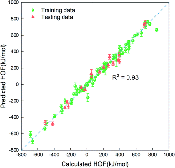
In order to quickly estimate the heat of formation for the unlabeled compounds in the vast search space, we need to construct a regressor based on the small amount of dataset labeled (88 representative compounds), which is an advantage of the PADF in the limited dataset. Due to the small-scale dataset, traditional machine learning methods are more appropriate than deep learning ones. Herein, we considered six machine learning algorithms (Lin, LASSO, KRR, SVR.lin, SVR.rbf, and GPR), which exhibited good performance in mapping the structure–property relationship for the small-scale dataset.29–33 As is known, the informative descriptors and efficient machine learning algorithms are critical to map the relationship between the descriptors and the targeted property. Thus, we tested the six traditional ML models and the four types of descriptors (SOB, ECFP, E-state and SOB + E-state) for the 88 initial samples labeled. Herein, “SOB + E-state” means the combination of the descriptor SOB (sum over bonds) and E-state (E-state fingerprint). Table 3 summaries predictive performances for 24 combinations for the 88 initial samples. As reflected in Table 3, ECFP coupled with the six regression models presents the worst performance. The six ML models coupled with the descriptor E-state characterizing the electrotopological state are poorer than those coupled with SOB. Judging from Rtest2, MAE and RMSE in Table 3, SVR.lin coupled with the combinatorial descriptor of SOB + E-state exhibits the best performance. Fig. 2 further shows high correlation between the heats of formation predicted by SVR.lin and ones calculated by the DFT method. Thus, SVR.lin coupled with the “SOB + E-state” descriptor is selected as the regressor to predict the heat of formation for the unexplored search space in the next step.
Table 3 Comparison of prediction accuracies between different combinations of the four types of descriptors and the six regression algorithms
| Modelsa |
Descriptors |
MAEtrainb |
MAEtestc |
RMSEtraind |
RMSEteste |
Rtrain2![[thin space (1/6-em)]](https://www.rsc.org/images/entities/char_2009.gif) f f |
Rtest2![[thin space (1/6-em)]](https://www.rsc.org/images/entities/char_2009.gif) g g |
| The ShuffleSplit method was used to divide the training set and the test set of 88 compounds (80% of the data set was used for the training set and 20% for the test set). The data set was divided 20 times in total to obtain the average value of the model evaluation index. Mean average error on the training set. Mean average error on the test set. Root mean squared error on the training set. Root mean squared error on the test set. Averaged R2 of the training set. Averaged R2 of the test set. |
| Lin |
SOB |
37.4 ± 2.0 |
68.2 ± 15.0 |
49.4 ± 2.5 |
87.7 ± 19.6 |
0.98 ± 0.00 |
0.92 ± 0.06 |
| ECFP |
18.7 ± 18.8 |
107.8 ± 44.4 |
24.7 ± 24.7 |
136.5 ± 54.8 |
0.99 ± 0.01 |
0.79 ± 0.16 |
| E-state |
34.8 ± 27.5 |
104.6 ± 37.7 |
44.4 ± 34.5 |
132.0 ± 47.4 |
0.97 ± 0.02 |
0.81 ± 0.15 |
| SOB + E-state |
33.5 ± 24.0 |
95.6 ± 37.4 |
43.2 ± 30.0 |
122.5 ± 46.4 |
0.98 ± 0.02 |
0.83 ± 0.14 |
| LASSO |
SOB |
39.2 ± 3.6 |
73.4 ± 20.5 |
50.6 ± 3.7 |
95.7 ± 30.2 |
0.98 ± 0.00 |
0.89 ± 0.12 |
| ECFP |
60.4 ± 32.3 |
115.7 ± 46.5 |
77.5 ± 41.6 |
144.7 ± 56.2 |
0.94 ± 0.06 |
0.76 ± 0.19 |
| E-state |
62.9 ± 26.7 |
109.6 ± 40.2 |
80.4 ± 34.3 |
137.6 ± 49.3 |
0.94 ± 0.05 |
0.78 ± 0.17 |
| SOB + E-state |
55.9 ± 26.2 |
98.5 ± 40.6 |
71.3 ± 33.7 |
124.5 ± 49.7 |
0.95 ± 0.05 |
0.82 ± 0.17 |
| KRR |
SOB |
35.9 ± 10.0 |
72.8 ± 13.4 |
46.0 ± 12.2 |
94.7 ± 18.3 |
0.98 ± 0.01 |
0.91 ± 0.07 |
| ECFP |
43.6 ± 135.8 |
195.3 ± 167.0 |
53.7 ± 165.2 |
242.4 ± 190.9 |
0.75 ± 1.03 |
0.12 ± 2.12 |
| E-state |
75.7 ± 13.3 |
105.0 ± 21.9 |
95.1 ± 15.0 |
132.4 ± 29.1 |
0.92 ± 0.03 |
0.81 ± 0.11 |
| SOB + E-state |
19.7 ± 8.0 |
64.1 ± 13.0 |
25.5 ± 10.0 |
85.0 ± 18.0 |
0.99 ± 0.00 |
0.92 ± 0.05 |
| SVR.lin |
SOB |
39.2 ± 4.5 |
66.6 ± 16.9 |
53.1 ± 3.1 |
86.4 ± 24.3 |
0.98 ± 0.00 |
0.92 ± 0.06 |
| ECFP |
11.0 ± 14.5 |
148.2 ± 22.1 |
15.1 ± 16.6 |
186.5 ± 28.6 |
1.00 ± 0.00 |
0.66 ± 0.12 |
| E-state |
69.0 ± 5.3 |
101.3 ± 19.7 |
87.6 ± 5.1 |
129.9 ± 30.7 |
0.94 ± 0.01 |
0.82 ± 0.12 |
| SOB + E-state |
32.7 ± 4.4 |
61.7 ± 15.3 |
45.4 ± 4.2 |
81.1 ± 19.1 |
0.98 ± 0.00 |
0.93 ± 0.06 |
| SVR.rbf |
SOB |
56.4 ± 14.9 |
134.6 ± 28.9 |
75.8 ± 13.6 |
170.2 ± 37.5 |
0.95 ± 0.02 |
0.70 ± 0.17 |
| ECFP |
172.5 ± 116.7 |
209.7 ± 81.8 |
213.6 ± 138.4 |
254.1 ± 92.0 |
0.48 ± 0.48 |
0.30 ± 0.44 |
| E-state |
150.9 ± 100.6 |
197.0 ± 72.5 |
188.8 ± 118.9 |
244.9 ± 82.9 |
0.60 ± 0.43 |
0.35 ± 0.43 |
| SOB + E-state |
124.8 ± 98.3 |
175.8 ± 74.1 |
157.6 ± 116.4 |
219.3 ± 86.0 |
0.69 ± 0.40 |
0.46 ± 0.43 |
| GPR |
SOB |
0.11 ± 0.01 |
110.3 ± 21.4 |
0.16 ± 0.02 |
149.3 ± 30.5 |
1.00 ± 0.00 |
0.76 ± 0.17 |
| ECFP |
0.06 ± 0.05 |
133.4 ± 33.6 |
0.10 ± 0.07 |
173.6 ± 40.8 |
1.00 ± 0.00 |
0.69 ± 0.17 |
| E-state |
0.08 ± 0.04 |
135.1 ± 32.7 |
0.12 ± 0.06 |
174.5 ± 40.5 |
1.00 ± 0.00 |
0.68 ± 0.19 |
| SOB + E-state |
0.09 ± 0.04 |
120.9 ± 38.2 |
0.13 ± 0.07 |
157.8 ± 47.1 |
1.00 ± 0.00 |
0.73 ± 0.19 |
 |
| | Fig. 2 The correlation between the average values predicted by SVR.lin coupled with E-state + SOB descriptors over 20 repeated tests and the heat of formation calculated at the level of CBS-4M. The training data and the testing data are represented by green spheres and orange triangles, respectively. | |
3.2 Combination of the regressor and the optimizer
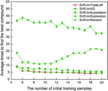
Although we can quickly estimate the heat of formation for the unexplored compounds in the vast search space using the regressor constructed, the regressor trained on the small-scale dataset labeled may suffer from large prediction uncertainty. Thus, it is a key question how to effectively select the desired compound from the vast search space. We hope that the compound has high heat of formation and can significantly improve the performance of the regressor when it is added into the initial training set. Consequently, the search needs to consider the ML-based prediction value and the uncertainty using an optimization function. Herein, we consider four optimization functions (exploitation, exploration, trade-off and KG). As mentioned in the section of Computational details, Exploitation selects the candidate with the maximum predicted value from the unknown search space while exploration selects the samples with the largest variance on the model predictions. The trade-off method is to balance the trade-off between exploitation and exploration to maximize the “expected improvement” (EI) while KG is similar to the trade-off between exploitation and exploration (see 2. Computational details). In addition, we also employ the random selection as a reference. In order to figure out the best optimization function, we test the performance of four optimization methods combined with SVR.lin as a function of the size of the training set. Specifically, the samples are randomly selected from the 88 labeled compounds as a training set in a given number (s = 5–20) while the remaining part of the 88 compounds acts as the search space. We use a combination pair of the SVR.lin regressor and each of the five optimizers to search the next compound from the search space, and count the number of iterations to find the compound with the highest heat of formation in the initial 88 samples. We repeat this process 1000 times for each initial set selected randomly with a specific number of samples ranging from 5 to 20, and calculate the average value of the number of iterations over the 1000 times.
The metric to evaluate the regressor/optimizer combination pair is the number of iterations required to find the best compound among the 88 samples labeled. Fig. 3 shows the performance of different regressor/optimizer combination pairs. It can be seen that the number of iterations gradually decreases with increasing number of the initial samples, except for exploration. Compared to the four optimizers, the random selection is the least efficient as it takes the most iteration times. Trade-off and KG that yield a compromise between exploration and exploitation show almost identical performance and are better than the other optimizers. As observed from Fig. 3, when the number of initial samples is beyond eight, the performance of SVR.lin/Trade-off and SVR.lin/KG becomes relatively stable. For the initial dataset containing eight samples, only five iterations are needed to find the optimal candidate from the remaining compounds, exhibiting high efficiency of the proposed PADF. Considering that SVR.lin/trade-off slightly outperforms SVR.lin/KG, the combination pair of SVR.lin/trade-off is finally determined to be the best combination pair, which will be used in searching the unknown space with more than eighty thousand samples.
 |
| | Fig. 3 Comparison of performance for the 10 regressor/optimizer combination pairs on different initial datasets randomly selected from the 88 samples labeled. The x axis represents the number of initial samples randomly selected from the 88 compounds to establish a statistical inference model. The y axis represents the average number of iterations required to find the best compound (i.e. the compound with the highest heat of formation) in the 88 samples. The standard deviation of the results over 20 repeated tests is marked by the error bar. The best regressor/optimizer combination pair is able to find the highly informative compound at the least number of iterations. The results show that the combination of SVR.lin/trade-off (vide the continuous red line) is the best regressor/optimizer pair. | |
3.3 Adaptive discovery for the target compound from the vast search space
After determining the best combination of the ML-based regressor and the optimizer, we apply them to select the desired compound with high heat of formation from the 83![[thin space (1/6-em)]](https://www.rsc.org/images/entities/char_2009.gif) 995 compounds unexplored in the search space. Specifically, SVR.lin is used to train the 88 samples labeled as the initial dataset, and applied to predict the heat of formation of the 83
995 compounds unexplored in the search space. Specifically, SVR.lin is used to train the 88 samples labeled as the initial dataset, and applied to predict the heat of formation of the 83![[thin space (1/6-em)]](https://www.rsc.org/images/entities/char_2009.gif) 995 unlabeled compounds in the search space. Fig. 4 shows the distribution of HOFs calculated by QM for the 88 samples. It can be seen that the HOF values of the initial dataset are not evenly distributed and samples with high heat of formation are relatively scarce. As is known, the regression models trained on the limited-scale and unbalanced dataset generally produce large prediction uncertainty and hardly avoid the local optimum. However, the optimization function could improve the predictive capacity of the regressor to the most extent through finding the highly informative sample to augment the training data with the aid of a self-adaptive cycle. For example, based on the EI scores obtained from the optimization function, the heat of formation of the beneficial compound selected from the unknown space would be calculated and added into the training set. Consequently, in the next iteration, the number of samples in the training set is increased to 89, while the prediction set contains 83
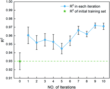
995 unlabeled compounds in the search space. Fig. 4 shows the distribution of HOFs calculated by QM for the 88 samples. It can be seen that the HOF values of the initial dataset are not evenly distributed and samples with high heat of formation are relatively scarce. As is known, the regression models trained on the limited-scale and unbalanced dataset generally produce large prediction uncertainty and hardly avoid the local optimum. However, the optimization function could improve the predictive capacity of the regressor to the most extent through finding the highly informative sample to augment the training data with the aid of a self-adaptive cycle. For example, based on the EI scores obtained from the optimization function, the heat of formation of the beneficial compound selected from the unknown space would be calculated and added into the training set. Consequently, in the next iteration, the number of samples in the training set is increased to 89, while the prediction set contains 83![[thin space (1/6-em)]](https://www.rsc.org/images/entities/char_2009.gif) 994 molecules. We continuously repeat the above process for the next round of the regression and selection. Consequently, the data distribution in the training set could be adjusted, in turn improving the learning ability of the regressor, as evidenced by Fig. 5. It can be seen that compared to the initial dataset containing 88 samples, R2 almost presents an upward trend as the number of samples with high heat of formation in the training set is increased by the iteration, despite some fluctuations within the ten iterations. All the iterations present higher R2 than original 88 training data. In addition, the standard deviation over the 20 repeated tests on every iteration is also lowered with increasing the number of iterations, as reflected by the error bar in Fig. 5, which implies an improvement in the prediction performance of the ML-model. The results clearly confirm that our self-adaptive strategy could efficiently improve the learning capacity of the regressor based on the small amount of training dataset to better map the relationship between the structure and the target property.
994 molecules. We continuously repeat the above process for the next round of the regression and selection. Consequently, the data distribution in the training set could be adjusted, in turn improving the learning ability of the regressor, as evidenced by Fig. 5. It can be seen that compared to the initial dataset containing 88 samples, R2 almost presents an upward trend as the number of samples with high heat of formation in the training set is increased by the iteration, despite some fluctuations within the ten iterations. All the iterations present higher R2 than original 88 training data. In addition, the standard deviation over the 20 repeated tests on every iteration is also lowered with increasing the number of iterations, as reflected by the error bar in Fig. 5, which implies an improvement in the prediction performance of the ML-model. The results clearly confirm that our self-adaptive strategy could efficiently improve the learning capacity of the regressor based on the small amount of training dataset to better map the relationship between the structure and the target property.
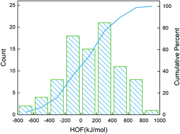 |
| | Fig. 4 Distribution of the heat of formation calculated at the level of CBS-4M for the 88 initial samples. The blue line denotes the cumulative percentage of the heat of formation. | |
 |
| | Fig. 5 The coefficient of determination R2 for the first ten iterations, derived from the SVR.lin regressor for 20 training and test sets obtained by the shuffle split method. Iteration 0 means that the training set is the initial 88 compounds, where the average value of R2 is 0.93. The standard deviation of the results over the 20 repeated tests is marked by the error bar for every iteration. | |
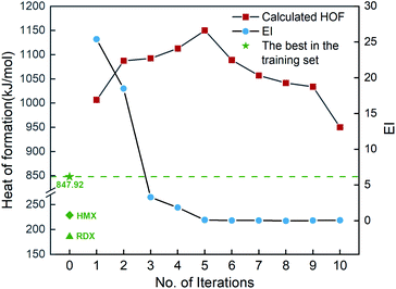
Fig. 6 shows the EI scores of the ten compounds selected at the first ten iterations by the SVR.lin/trade-off combination pair. It can be seen that the EI score keeps a downward trend before the 5th iteration. After that, the EI scores approach an equilibrium. Fig. 6 also displays the calculated heat of formation by QM for the compound selected at each iteration. It can be seen that the heat of formation presents to some extent fluctuation with increasing number of iterations. The heat of formation reaches a peak value (1150.08 kJ mol−1) at iteration 5, and then drops in subsequent iterations. It can be seen that the ten compounds selected from the unexplored space at the first ten iterations all present higher values than the maximum one (847.92 kJ mol−1) of the initial training set containing 88 compounds and those of the two classic explosives HMX and RDX. The result clearly shows that our PADF can quickly search the energetic compounds with high heat of formation from the vast unknown space, only needing several iterations.
 |
| | Fig. 6 The heat of formation calculated by CBS-4M and EI scores of the ten compounds selected by the SVR.lin/trade-off combination pair. Iteration 0 means that the training set is the initial 88 compounds, where the maximum value of the heat of formation is 847.92 kJ mol−1. For each iteration (starting from 1), a new compound will be selected from the remaining unexplored space and verified by the CBS-4M calculation. Then it is added to the training set for the next iteration (see 2. Computational details). | |
Chart 1 presents the 2D structure and molecular formula of the ten compounds (a1–a10) selected from the first 10 iterations. Comparing the ten compounds selected, it can be seen that they all include the substituent of –NHNO2, except for the compound a9. In addition, eight compounds, except for a1 and a10, possess the same parent ring, i.e., 6-(1H-pyrazole-4-amino)-[1,2,4]azole[4,3-b]-1,2,4,5-tetrazine, indicating the highly energetic property of the parent ring. The substituted sites of the substituents are the same for the compounds a5 and a6, but the heat of formation of a5 substituted by two –NHNO2 is higher than that of the compound a6 substituted by one –NHNO2 and –ONO2, indicating higher energetic potential of the substituent –NHNO2 than –ONO2 for the heat of formation. The compound a1 was synthesized by Fischer and considered to be a promising powerful explosive, judging from some computational evidence.46 The heat of formation of the parent ring of a10 was calculated to be 164.56 kJ mol−1 by Bo,47 much lower than that of a10 (949.87 kJ mol−1) substituted by two –NHNO2. The heat of formation of the compound with the same parent ring as a2–a9 but with two –NO2 substituted at the carbon atom of pyrazole was reported to be 550.84 kJ mol−1,48 significantly lower than those of the eight compounds (a2–a9) with the same parent ring, indicating the energetic characteristics of the –NHNO2 and –ONO2 substituents.
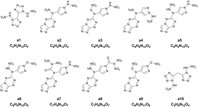 |
| | Chart 1 The 2D structures and molecular formulas of the ten compounds (a1–a10) selected from the first ten iterations for the heat of formation as the target property. | |
3.4 Detonation performance
To further evaluate the detonation performance of the ten compounds selected from our PADF, we calculate several detonation properties, i.e., the oxygen balance, the detonation velocity and the detonation pressure. The calculated results are summarized in Table 4, along with the corresponding properties of the two classic explosives RDX and HMX. The two explosives generally serve as the benchmark for HEDMs.25 It can be seen that the ten compounds selected are significantly higher than RDX and HMX for the heat of formation. However, their detonation velocities and detonation pressures are lower than those of the two classic explosives. Furthermore, their oxygen balances are also lower than those of HMX and RDX, except for a1. The compound a5 possesses the highest heat of formation, but its oxygen balance, detonation velocity and detonation pressure are in the last second order of the ten compounds, much lower than those of RDX and HMX. In contrast, the compound a1 with the heat of formation in the last second order outperforms RDX and is close to HMX for the detonation velocity and pressure, and its oxygen balance is close to zero. The observation indicates that the heat of formation cannot well reflect the detonation performance of the explosives. Generally, the energetic materials require not only excellent detonation properties, but also thermal stabilities, which is associated with the safety in practical applications. As accepted, the bond dissociation energy (BDE) is related to the thermal stability. Thus, we also calculate BDEs of the ten compounds and the two classic explosives, as shown in Table 4. It was proposed that if the bond dissociation energy is greater than 80 kJ mol−1, the compound meets the basic requirements for the stability of the energetic compound; if it is greater than 120 kJ mol−1, then the energetic compound possesses excellent stability.49 Judging from the rules, the compounds a1, a4, a5, a7 and a10 are thermally stable.
Table 4 The detonation performance of compounds a1–a10 selected from the heat of formation as the target property and two classic explosives
| Compounds |
ΔHfa (kJ mol−1) |
OBb (%) |
Dc (m s−1) |
Pd (GPa) |
BDEe (kJ mol−1) |
| Heat of formation (kJ mol−1). Oxygen balance (%). Detonation velocity (m s−1). Detonation pressure (GPa). Bond dissociation energy (kJ mol−1). The values were calculated using the same method as the ten compounds. The experimental values were obtained from a literature study.41 |
| a1 |
1006.68 |
−6.20 |
9113.69 |
37.10 |
103.54 |
| a2 |
1087.55 |
−51.92 |
8381.64 |
31.55 |
64.37 |
| a3 |
1092.59 |
−44.42 |
8428.66 |
32.03 |
28.55 |
| a4 |
1112.74 |
−74.77 |
7789.38 |
26.60 |
97.55 |
| a5 |
1150.08 |
−51.98 |
8142.99 |
29.42 |
95.29 |
| a6 |
1088.93 |
−44.42 |
8377.83 |
31.49 |
26.84 |
| a7 |
1057.16 |
−36.35 |
8434.83 |
32.22 |
92.01 |
| a8 |
1041.62 |
−36.35 |
8348.48 |
31.35 |
79.18 |
| a9 |
1033.76 |
−36.90 |
8762.72 |
34.76 |
28.61 |
| a10 |
949.87 |
−23.52 |
8822.93 |
34.80 |
114.36 |
| RDX |
Calcf |
185.73 |
−21.61 |
9047.12 |
36.20 |
140.79 |
| Expg |
— |
— |
8750 |
34.00 |
— |
| HMX |
Calcf |
228.78 |
−21.61 |
9247.75 |
38.93 |
164.40 |
| Expg |
— |
— |
9100 |
39.00 |
— |
3.5 Generalization of the PADF to search energetic compounds with high heat of explosion
To evaluate the generalization capacity of the PADF for other target properties, we extend it to the heat of explosion as the desired property. The heat of explosion of each initial sample is calculated in terms of the methods listed in Table 2. Similarly, we test different descriptors, regression models and optimizers in order to construct the best PADF for the heat of explosion. In the case of HOF, the ECFP descriptor presents the poorest performance in the regression model while the SOB coupled with E-state performs best. Thus, in the part, we exclude the ECFP descriptor. However, as reflected by Table S4 in the ESI,† SOB, E-state and SOB + E-state used in the heat of formation all exhibit poor prediction accuracies, indicating that these descriptors do not completely characterize features associated with the heat of explosion. Thereby, we add another type of descriptor called the custom descriptor set (CDS). The CDS includes fifteen kinds of features involving the types of N and O atoms and elementary composition. The N and O atoms are categorized according to how they incorporate into a molecule, including C–NO2, N–NO2, O–N![[double bond, length as m-dash]](https://www.rsc.org/images/entities/char_e001.gif) O, O–NO2, C–N
O, O–NO2, C–N![[double bond, length as m-dash]](https://www.rsc.org/images/entities/char_e001.gif) N, C
N, C![[double bond, length as m-dash]](https://www.rsc.org/images/entities/char_e001.gif) N–O, C–NH2 and N–O–C, which are not involved in SOB. In addition, the CDS also includes oxygen balance, counts of N, C and H, and the ratio between nitrogen and carbon atoms. These features are considered to be associated with the explosion process.50 As shown in Table S4 and Fig. S1 in the ESI,† the combinatorial descriptor E-state + SOB + CDS coupled with the KRR model outperforms other descriptors like SOB, E-state, CDS, and SOB + E-state for the test set. Its prediction accuracy reaches 0.90Rtest2 with 69.5 cal g−1 MAEtest.
N–O, C–NH2 and N–O–C, which are not involved in SOB. In addition, the CDS also includes oxygen balance, counts of N, C and H, and the ratio between nitrogen and carbon atoms. These features are considered to be associated with the explosion process.50 As shown in Table S4 and Fig. S1 in the ESI,† the combinatorial descriptor E-state + SOB + CDS coupled with the KRR model outperforms other descriptors like SOB, E-state, CDS, and SOB + E-state for the test set. Its prediction accuracy reaches 0.90Rtest2 with 69.5 cal g−1 MAEtest.
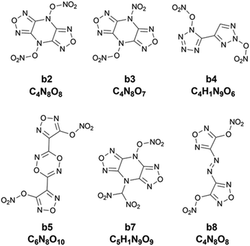
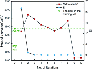
In addition, the combination of KRR/KG is found to be the best combination of the regressor and the optimizer, evidenced by Fig. S2 in the ESI.† Then ten iterative loops are conducted to search the unknown space with more than eighty thousand compounds, using the KRR/KG combination. Fig. 7 depicts the iteration results. It can be seen that there are six selected compounds (i.e. b2, b3, b4, b5, b7 and b8) within the first ten iterations presenting higher heat of explosion than the highest one (1775.19 cal g−1) among the initial 88 samples in the training set, exhibiting good performance. However, compared to the heat of formation above, the search performance is lower. For the heat of formation, all the ten compounds selected are superior to the one with the highest value among the initial samples. As shown in Table S4,† the determination coefficient on the test set Rtest2 of the heat of explosion is 0.90 ± 0.05, lower than the heat of formation (0.93 ± 0.06). The observation indicates that the ML-based prediction on the heat of explosion has relatively larger uncertainty (i.e. variance) than that on the heat of formation. Consequently, there are relatively more compounds selected that are inferior to the best compound of the initial dataset, compared to the heat of formation. The result indicates that the prediction performance of the ML-based regressor could influence the search efficiency of the optimizers like trade-off and KG used in our PADF. It is not unexpected since the trade-off and KG optimizer are based on maximizing the “expected improvement” (EI) that takes both the average prediction value (μ) and uncertainty (σ) into consideration. The lower the ML model prediction performance the larger the prediction uncertainty. In order to maximize the EI value, the optimizer tends to select samples with large uncertainty from the search space, as reflected by eqn (5) and (6). The adaptive design strategy also hopes to add the compound with large uncertainty to the training set so that the prediction performance of the ML models could be efficiently improved through further training.20 To confirm the search efficiency of the PADF, we continuously conduct 40 iterations after the first ten iterations, as shown in Fig. S3.† It can be seen that the heat of explosion of the selected compounds almost presents a downward trend for the first 50 iterations despite some fluctuations. Furthermore, the heats of explosion of the latter 40 selected compounds are lower than the maximum value of the first 10 iterations (1940.71 cal g−1). It further confirms that our PADF can quickly screen high-performing samples from the unknown search space in very few iterations. It is noted that if the ML-based regressor has higher prediction accuracy, there would be more compounds selected with better properties than the initial training set.
 |
| | Fig. 7 The heat of explosion derived from the QM calculation and empirical equation and EI scores of 10 compounds selected by the KRR/KG combination pair. Iteration 0 means that the training set consists of the initial 88 compounds, where the maximum value of the heat of explosion is 1775.19 cal g−1. For each iteration (starting from 1), a new compound will be selected from the remaining unexplored space and further verified by the QM-based evaluation system, which will be added into the training set for the next iteration (see 2. Computational details). | |
Chart 2 shows 2D structures of the six compounds. A comparison of chemical structures between the six compounds and the ten compounds a1–a10 selected from the heat of formation clearly shows that they are completely different in either parent rings or substituents. The six compounds derived from the heat of explosion commonly contain substituents –ONO2 and –NO2, and do not have the –NHNO2 group existing in the compounds a1–a10. In some literature studies involving energetic materials, the heats of explosion of compounds with the same parent ring as b2, b3 and b7 but with the two substituents –CH2ONO2 and two substituents –NHNO2 at the same substitution site were reported to be 1540.86 cal g−1 and 1651.21 cal g−1,51,52 respectively, whereas the lowest heat of explosion of the b2, b3 and b7 compounds is 1786.43 cal g−1. The heat of explosion of the compound with the same parent ring as b4 but with one –NO2 substituted at the triazole ring was reported to be 1253.57 cal g−1,53 significantly lower than the 1821.60 cal g−1 of b4. The compound, which has an identical parent ring and substitution site to b5 but substituted by two –NHNO2 (rather than the two –ONO2 like b5), was reported to have 1545.21 cal g−1 for heat of explosion,54 lower than the 1791.24 cal g−1 of b5. The heat of explosion of the compound with the same parent ring as b8 but substituted by two –CH(NO2)2 was reported to be 1622.42 cal g−1,55 significantly lower than that of b8 substituted by two –ONO2 (Q: 1869.22 cal g−1). These observations show the high energetic performance of –ONO2 for the heat of explosion.
 |
| | Chart 2 The 2D structure and molecular formula of the six compounds (b2, b3, b4, b5, b7 and b8) with higher heat of explosion than the maximum value of the initial 88 compounds. | |
Table 5 also lists the detonation performance calculated for the six compounds. Compared to the two classic explosives HMX and RDX, the six compounds exhibit higher heat of explosion. Furthermore, their oxygen balances are also better than those of HMX and RDX. Except for b8, the other five compounds have higher detonation velocities and detonation pressures than HMX and RDX. These observations indicate that the heat of explosion as the target property could better select compounds with high detonation performance than the heat of formation. However, except for b3, BDEs of the other five compounds are much lower than 80 kJ mol−1, exhibiting low thermal instability. Interestingly, the compound b3 not only has higher detonation performance than HMX and RDX, but also presents excellent thermal stability with 141.33 kJ mol−1 for BDE, exhibiting high potential as a new explosive with high performance.
Table 5 The detonation performance of six compounds selected from the heat of explosion as the target property and two classic explosives HMX and RDX
| Compounds |
Qa (cal g−1) |
OBb (%) |
Dc (m s−1) |
Pd (GPa) |
BDEe (kJ mol−1) |
| Heat of explosion (cal g−1). Oxygen balance (%). Detonation velocity (m s−1). Detonation pressure (GPa). Bond dissociation energy (kJ mol−1). The values were calculated using the same method as the six compounds. The experimental values were obtained from a literature study.41 |
| b2 |
1940.71 |
0.00 |
9567.64 |
42.17 |
54.05 |
| b3 |
1889.24 |
−5.88 |
9414.28 |
40.76 |
141.33 |
| b4 |
1821.60 |
−3.09 |
9441.44 |
40.63 |
34.43 |
| b5 |
1791.24 |
−9.30 |
9096.66 |
37.92 |
14.37 |
| b7 |
1786.43 |
−7.25 |
9298.34 |
39.75 |
26.22 |
| b8 |
1869.22 |
0.00 |
8983.56 |
35.56 |
28.36 |
| RDX |
Calcf |
1553.89 |
−21.61 |
9047.12 |
36.20 |
140.79 |
| Expg |
— |
— |
8750 |
34.00 |
— |
| HMX |
Calcf |
1549.78 |
−21.61 |
9247.75 |
38.93 |
164.40 |
| Expg |
— |
— |
9100 |
39.00 |
— |
4 Conclusions
In this work, we developed a property-oriented adaptive design framework to quickly discover the target molecule from the vast space unexplored in the case of limited scale datasets available. The performance of the design framework is validated by two case studies on discovering energetic materials with high heat of formation and high heat of explosion. The framework proposed is composed of a ML-based regressor, an optimizer and a validation system based on quantum mechanics calculations. We only utilized around 0.1% (88 samples) of the vast unexplored space as the initial dataset to label their properties. Based on the small dataset labeled, the machine learning model is trained to obtain the regressor in order to predict the target property for the remaining compounds in the vast search space. Then different optimization algorithms are used to help select the high-performing compound from the search space. Tests on different combination pairs of the regressors and the optimizers indicate that the best pairs are SVR.lin/Trade-off coupled with E-state + SOB descriptors for the heat of formation and KRR/KG coupled with CDS + E-state + SOB descriptors for the heat of explosion. Most of the selected compounds within the first ten iterations present better performance in the target property than the initial dataset. For these selected compounds, we also further evaluated their oxygen balances, detonation velocities, detonation pressures and bond dissociation energies, which are closely associated with the detonation performance and the thermal stability of the explosives. The results show that the compounds selected from the two different target properties are completely different, either in the parent ring or in the substituent. The substituent –NHNO2 favors the high heat of formation, but disfavors the high heat of explosion. The substituent –ONO2 exhibits an advantage in improving the heat of explosion. Furthermore, the heat of explosion as the target property outperforms the heat of formation in designing new explosives with high detonation performance. Also, it is worthy of note that the compound b3 selected at the 3rd iteration based on the heat of explosion exhibits better performance (heat of explosion: 1889.24 cal g−1, detonation velocity: 9414.28 m s−1, detonation pressure: 40.76 GPa and oxygen balance: −5.88%) than the two benchmark explosives RDX and HMX. Furthermore, the bond dissociation energy calculation further indicates that the compound b3 has excellent thermal stability. These lines of evidence demonstrate the high potential of the compound b3 as a low-sensitivity HEDM. The observations indicate that our PADF constructed can quickly design energetic compounds with desired properties. The successful application of the PADF in the two cases confirms its generalization ability, indicating that the design framework could be extended to other fields limited by the small-scale labeled dataset. Despite the encouraging results, our findings still need further experimental validation.
Author contributions
Yunhao Xie: conceptualization, formal analysis, and writing – original draft preparation. Yijing Liu: methodology and software. Renling Hu: formal analysis and validation. Xu Lin: investigation and visualization. Jing Hu: data curation. Xuemei Pu: supervision and writing – reviewing.
Conflicts of interest
There are no conflicts to declare.
Acknowledgements
This project was supported by NSAF (Grant no. U1730127), Sichuan International Science and Technology Innovation Cooperation Project (Grant no. 2021YFH0140) and Key Laboratory Foundation (Grant no. 6142603190305).
Notes and references
- R. Dehghannasiri, D. Xue, P. V. Balachandran, M. R. Yousefi, L. A. Dalton, T. Lookman and E. R. Dougherty, Comput. Mater. Sci., 2017, 129, 311–322 CrossRef CAS.
- D. Dey, P. J. Slomka, P. Leeson, D. Comaniciu, S. Shrestha, P. P. Sengupta and T. H. Marwick, J. Am. Coll. Cardiol., 2019, 73, 1317–1335 CrossRef PubMed.
- X. Yang, Y. Wang, R. Byrne, G. Schneider and S. Yang, Chem. Rev., 2019, 119, 10520–10594 CrossRef CAS PubMed.
- H. Wang, Y. Ji and Y. Li, Wiley Interdiscip. Rev.: Comput. Mol. Sci., 2020, 10, e1421 CAS.
- J. Zeng, L. Cao, M. Xu, T. Zhu and J. Z. Zhang, Nat. Commun., 2020, 11, 1–9 Search PubMed.
- G. Li and C. Zhang, J. Hazard. Mater., 2020, 122910 CrossRef CAS PubMed.
- Y. Liu, G. Zhao, Q. Yu, Y. Tang, G. H. Imler, D. A. Parrish and J. M. Shreeve, J. Org. Chem., 2019, 84, 16019 CrossRef CAS PubMed.
- Y. Qu, Q. Zeng, J. Wang, Q. Ma, H. Li, H. Li and G. Yang, Chem.–Eur. J., 2016, 22, 12527 CrossRef CAS PubMed.
- J. Zhang, B. Jin, R. Peng, C. Niu, L. Xiao, Z. Guo and Q. Zhang, Dalton Trans., 2019, 48, 11848 RSC.
- Y. Wang, Y. Liu, S. Song, Z. Yang, X. Qi, K. Wang, Y. Liu, Q. Zhang and Y. Tian, Nat. Commun., 2018, 9, 2444 CrossRef PubMed.
- M. Jaidann, S. Roy, H. Abou-Rachid and L.-S. Lussier, J. Hazard. Mater., 2010, 176, 165–173 CrossRef CAS PubMed.
- X. Li, Q. Sun, Q. Lin and M. Lu, Chem. Eng. J., 2021, 406, 126817 CrossRef CAS.
- W. Zhao, S. J. Carey, Z. Mao and C. T. Campbell, ACS Catal., 2018, 8, 1485–1489 CrossRef CAS.
- M. Fathollahi and H. Sajady, J. Therm. Anal. Calorim., 2018, 133, 1663–1672 CrossRef CAS.
- A. Al-Fakih, Z. Algamal, M. Lee and M. Aziz, SAR QSAR Environ. Res., 2018, 29, 339–353 CrossRef CAS PubMed.
- M. H. Keshavarz, M. Jafari, K. Esmaeilpour and M. Samiee, Process Saf. Environ. Prot., 2018, 113, 491–497 CrossRef CAS.
- T. L. Jensen, J. F. Moxnes, E. Unneberg and D. Christensen, J. Mol. Model., 2020, 26, 1–14 CrossRef PubMed.
- N. Zohari, F. Abrishami and V. Zeynali, Z. Anorg. Allg. Chem., 2017, 643, 2124–2137 CrossRef CAS.
- Y. Wang, Q. Yao, J. T. Kwok and L. M. Ni, ACM Comput. Surv., 2020, 53, 63 Search PubMed.
- H. A. Doan, G. Agarwal, H. Qian, M. J. Counihan, J. Rodríguez-López, J. S. Moore and R. S. Assary, Chem. Mater., 2020, 32, 6338–6346 CrossRef CAS.
- C. Wen, Y. Zhang, C. Wang, D. Xue, Y. Bai, S. Antonov, L. Dai, T. Lookman and Y. Su, Acta Mater., 2019, 170, 109–117 CrossRef CAS.
- R. Yuan, Z. Liu, P. V. Balachandran, D. Xue, Y. Zhou, X. Ding, J. Sun, D. Xue and T. Lookman, Adv. Mater., 2018, 30, 1702884 CrossRef PubMed.
- G. P. Nagabhushana, R. Shivaramaiah and A. Navrotsky, Proc. Natl. Acad. Sci. U. S. A., 2016, 113, 7717–7721 CrossRef CAS PubMed.
- D. H. Zaitsau and S. P. Verevkin, J. Mol. Liq., 2019, 287, 110963 CrossRef.
- O. T. O'Sullivan and M. J. Zdilla, Chem. Rev., 2020, 120, 5682–5744 CrossRef PubMed.
- K. Hansen, F. Biegler, R. Ramakrishnan, W. Pronobis, O. A. Von Lilienfeld, K.-R. Müller and A. Tkatchenko, J. Phys. Chem. Lett., 2015, 6, 2326–2331 CrossRef CAS PubMed.
- D. Rogers and M. Hahn, J. Chem. Inf. Model., 2010, 50, 742–754 CrossRef CAS PubMed.
- L. H. Hall and L. B. Kier, J. Chem. Inf. Comput. Sci., 1995, 35, 1039–1045 CrossRef CAS.
- X. Shen, W. Pan and Y. Zhu, J. Am. Stat. Assoc., 2012, 107, 223–232 CrossRef PubMed.
- G. H. Gu, P. Plechac and D. G. Vlachos, React. Chem. Eng., 2018, 3, 454–466 RSC.
- P. R. Regonia, C. M. Pelicano, R. Tani, A. Ishizumi, H. Yanagi and K. Ikeda, Optik, 2020, 207, 164469 CrossRef CAS.
- A. Alzghoul, A. Alhalaweh, D. Mahlin and C. A. Bergström, J. Chem. Inf. Model., 2014, 54, 3396–3403 CrossRef CAS PubMed.
- E. Swinnich, Y. J. Dave, E. B. Pitman, S. Broderick, B. Mazumder and J.-H. Seo, Mater. Discovery, 2018, 11, 1–5 CrossRef.
- F. Pedregosa, G. Varoquaux, A. Gramfort, V. Michel, B. Thirion, O. Grisel, M. Blondel, P. Prettenhofer, R. Weiss and V. Dubourg, J. Mach. Learn. Res., 2011, 12, 2825–2830 Search PubMed.
- D. R. Jones, M. Schonlau and W. J. Welch, J. Global. Optim., 1998, 13, 455–492 CrossRef.
- L. A. Curtiss, K. Raghavachari, P. C. Redfern and J. A. Pople, J. Chem. Phys., 1997, 106, 1063–1079 CrossRef CAS.
- D. Fischer, T. M. Klapötke, M. Reymann and J. Stierstorfer, Chem.–Eur. J., 2014, 20, 6401–6411 CrossRef CAS PubMed.
- M. Göbel, K. Karaghiosoff, T. M. Klapötke, D. G. Piercey and J. r. Stierstorfer, J. Am. Chem. Soc., 2010, 132, 17216 CrossRef PubMed.
- P. J. Linstrom and W. G. Mallard, J. Chem. Eng. Data, 2001, 46, 1059–1063 CrossRef CAS.
- M. J. Kamlet and S. Jacobs, J. Chem. Phys., 1968, 48, 23–35 CrossRef CAS.
- P. Politzer and J. S. Murray, Cent. Eur. J. Energ. Mater., 2011, 8, 209–220 CAS.
- P. Politzer, J. Martinez, J. S. Murray, M. C. Concha and A. Toro-Labbe, Mol. Phys., 2009, 107, 2095–2101 CrossRef CAS.
- T. Lu and F. Chen, J. Comput. Chem., 2012, 33, 580–592 CrossRef CAS PubMed.
- P. Politzer and J. S. Murray, J. Mol. Struct., 1996, 376, 419–424 CrossRef CAS.
- M. J. Frisch, G. W. Trucks, H. B. Schlegel, G. E. Scuseria, M. A. Robb, J. R. Cheeseman, G. Scalmani, V. Barone, B. Mennucci, G. A. Petersson, H. Nakatsuji, M. Caricato, X. Li, H. P. Hratchian, A. F. Izmaylov, J. Bloino, G. Zheng, J. L. Sonnenberg, M. Hada, M. Ehara, K. Toyota, R. Fukuda, J. Hasegawa, M. Ishida, T. Nakajima, Y. Honda, O. Kitao, H. Nakai, T. Vreven, J. E. Peralta, F. Ogliaro, M. Bearpark, J. J. Heyd, E. Brothers, K. N. Kudin, V. N. Staroverov, R. Kobayashi, J. Normand, K. Raghavachari, A. Rendell, J. C. Burant, S. S. Iyengar, J. Tomasi, M. Cossi, N. Rega, J. M. Millam, M. Klene, J. E. Knox, J. B. Cross, V. Bakken, C. Adamo, J. Jaramillo, R. Gomperts, R. E. Stratmann, O. Yazyev, A. J. Austin, R. Cammi, C. Pomelli, J. W. Ochterski, R. L. Martin, K. Morokuma, V. G. Zakrzewski, G. A. Voth, P. Salvador, J. J. Dannenberg, S. Dapprich, A. D. Daniels, Ö. Farkas, J. B. Foresman, J. V. Ortiz, J. Cioslowski and D. J. Fox. Gaussian. Inc., Wallingford, CT, 2009.
- D. Fischer, T. M. Klapötke, J. Stierstorfer and N. Szimhardt, Chem.–Eur. J., 2016, 22, 4966–4970 CrossRef CAS PubMed.
- Z. Bo, C. Sitong, G. Weiming, Z. Weijing, W. Lin, Y. Li and Z. Jianguo, Sci. Rep., 2017, 7, 13426 CrossRef PubMed.
- V. Sinditskii, S. Smirnov, V. Y. Egorshev, A. Chernyi, T. Shkineva, N. Palysaeva, K. Y. Suponitsky and I. Dalinger, Thermochim. Acta, 2017, 651, 83–99 CrossRef CAS.
- Z. X. Chen and H. M. Xiao, Propellants, Explos., Pyrotech., 2014, 39, 487–495 CrossRef CAS.
- D. C. Elton, Z. Boukouvalas, M. S. Butrico, M. D. Fuge and P. W. Chung, Sci. Rep., 2018, 8, 9059 CrossRef PubMed.
- W. Li, K. Wang, X. Qi, Y. Jin and Q. Zhang, Cryst. Growth Des., 2018, 18, 1896–1902 CrossRef CAS.
- J. Zhang, P. Yin, L. A. Mitchell, D. A. Parrish and M. S. Jean'Ne, J. Mater. Chem. A, 2016, 4, 7430–7436 RSC.
- D. Izsák, T. M. Klapötke and C. Pflüger, Dalton Trans., 2015, 44, 17054–17063 RSC.
- H. Huang, Y. Shi, Y. Liu and J. Yang, Dalton Trans., 2016, 45, 15382–15389 RSC.
- Y. Tang, H. Gao, G. H. Imler, D. A. Parrish and M. S. Jean'ne, RSC Adv., 2016, 6, 91477–91482 RSC.
Footnote |
| † Electronic supplementary information (ESI) available: Table S1: the Chemical structures and SMILES (simplified molecular input line entry specification) of 88 parent rings. Table S2: the chemical structures and SMILES of 13 substituents. Table S3: the chemical structures and descriptor matrix of 88 initial compounds. Table S4: comparison of prediction accuracies for different combinations of five types of descriptors and six regression algorithms for the heat of explosion as the target property. Fig. S1: the relationship between the average values predicted by KRR coupled with E-state + SOB + CDS for 20 repeated tests and calculated values derived from the QM method and empirical equation for the heat of explosion. Fig. S2: comparison of performance for the 10 regressor/optimizer combination pairs on different initial dataset randomly selected from the 88 samples labeled for the heat of explosion, derived from 20 repeated tests. Fig. S3: the calculated heat of explosion derived from the QM calculation and empirical equation of 50 compounds selected from the first 50 iterations by means of the KRR/KG combination pair. See DOI: 10.1039/d1ra03715c |
|
| This journal is © The Royal Society of Chemistry 2021 |
Click here to see how this site uses Cookies. View our privacy policy here.  Open Access Article
 a,
Yijing Liub,
Renling Hua,
Xu Lina,
Jing Hua and
Xuemei Pu
 *a
*a
![[thin space (1/6-em)]](https://www.rsc.org/images/entities/char_2009.gif) 083 compounds generated. SVR.lin/Trade-off coupled with E-state + SOB and KRR/KG coupled with CDS + E-state + SOB were determined to be the best combination pairs for the heat of formation and the heat of explosion, respectively. Most of the ten compounds selected from the first ten iterations exhibit better properties than the optimal sample in the initial dataset. Besides, the heat of explosion as the target property outperforms the heat of formation in designing energetic compounds with high detonation performance. In particular, a new compound selected at the 3rd iteration exhibits high potential as an explosive. Our strategy could be extended to other domains limited by small-scale datasets labeled.
083 compounds generated. SVR.lin/Trade-off coupled with E-state + SOB and KRR/KG coupled with CDS + E-state + SOB were determined to be the best combination pairs for the heat of formation and the heat of explosion, respectively. Most of the ten compounds selected from the first ten iterations exhibit better properties than the optimal sample in the initial dataset. Besides, the heat of explosion as the target property outperforms the heat of formation in designing energetic compounds with high detonation performance. In particular, a new compound selected at the 3rd iteration exhibits high potential as an explosive. Our strategy could be extended to other domains limited by small-scale datasets labeled.![[thin space (1/6-em)]](https://www.rsc.org/images/entities/char_2009.gif) 083 samples, including 2944 mono-substituted compounds and 81
083 samples, including 2944 mono-substituted compounds and 81![[thin space (1/6-em)]](https://www.rsc.org/images/entities/char_2009.gif) 139 di-substituted compounds.
139 di-substituted compounds.
![[thin space (1/6-em)]](https://www.rsc.org/images/entities/char_2009.gif) 139); (3) based on the former two rules, the total number of each substituent appearing in the initial dataset is determined to be twelve or thirteen to ensure the representativity of each substituent. Consequently, the initial dataset was composed of 88 compounds. Their 3D structures were obtained using Simplified Molecular Input Line Entry System (SMILES) strings with the RDKit library.
139); (3) based on the former two rules, the total number of each substituent appearing in the initial dataset is determined to be twelve or thirteen to ensure the representativity of each substituent. Consequently, the initial dataset was composed of 88 compounds. Their 3D structures were obtained using Simplified Molecular Input Line Entry System (SMILES) strings with the RDKit library.
![[thin space (1/6-em)]](https://www.rsc.org/images/entities/char_2009.gif) 083 compounds: N
083 compounds: N![[double bond, length as m-dash]](https://www.rsc.org/images/entities/char_e001.gif) N, N
N, N![[double bond, length as m-dash]](https://www.rsc.org/images/entities/char_e001.gif) O, C:N, C:O, C:C, C–O, C–N, C–H, C–C, C/C, N:O, N:N, C/O, C/N, N/N, O–O, C
O, C:N, C:O, C:C, C–O, C–N, C–H, C–C, C/C, N:O, N:N, C/O, C/N, N/N, O–O, C![[double bond, length as m-dash]](https://www.rsc.org/images/entities/char_e001.gif) O, C
O, C![[double bond, length as m-dash]](https://www.rsc.org/images/entities/char_e001.gif) N, H–N, N–N, N–O, C
N, H–N, N–N, N–O, C![[double bond, length as m-dash]](https://www.rsc.org/images/entities/char_e001.gif) C (‘–’ for single bond, ‘
C (‘–’ for single bond, ‘![[double bond, length as m-dash]](https://www.rsc.org/images/entities/char_e001.gif) ’ for double bond, ‘/’ for directional bond and ‘:’ for aromatic bond).
’ for double bond, ‘/’ for directional bond and ‘:’ for aromatic bond).![[thin space (1/6-em)]](https://www.rsc.org/images/entities/char_2009.gif) 083 compounds only involve thirteen atom types, so we threw out the vectors that are always zero and truncated the descriptors to a length of thirteen.
083 compounds only involve thirteen atom types, so we threw out the vectors that are always zero and truncated the descriptors to a length of thirteen.![[thin space (1/6-em)]](https://www.rsc.org/images/entities/char_2009.gif) 083 compounds generated, there are seven types of N and three types of O, such as C–NO2, N–NO2, O–N
083 compounds generated, there are seven types of N and three types of O, such as C–NO2, N–NO2, O–N![[double bond, length as m-dash]](https://www.rsc.org/images/entities/char_e001.gif) O, O–NO2, C–N
O, O–NO2, C–N![[double bond, length as m-dash]](https://www.rsc.org/images/entities/char_e001.gif) N, C
N, C![[double bond, length as m-dash]](https://www.rsc.org/images/entities/char_e001.gif) N–O, C–NH2, N–O–C, N
N–O, C–NH2, N–O–C, N![[double bond, length as m-dash]](https://www.rsc.org/images/entities/char_e001.gif) O and C
O and C![[double bond, length as m-dash]](https://www.rsc.org/images/entities/char_e001.gif) O. The number of each type is counted. In addition to the ten descriptors, CDS also includes oxygen balance, counts of N, C and H, and the ratio between nitrogen and carbon atoms.
O. The number of each type is counted. In addition to the ten descriptors, CDS also includes oxygen balance, counts of N, C and H, and the ratio between nitrogen and carbon atoms.


 is the sum of calculated heat of formation over all atoms at 298 K and
  is the sum of the experimental values of standard heat of formation over all atoms at 298 K. To use the atomization energy method to calculate the heat of formation for the energetic compounds, it is necessary to acquire the data of the standard heat of formation of each atom at 298 K. Table 1 lists the heat of formation values of the C, H, O and N atoms, derived from CBS-4M methods and the experiment.39
 and the experimental determination
![[M with combining macron]](https://www.rsc.org/images/entities/i_char_004d_0304.gif) ) for the energetic compound CaHbOcNda
) for the energetic compound CaHbOcNda


![[M with combining macron]](https://www.rsc.org/images/entities/i_char_004d_0304.gif)


![[M with combining macron]](https://www.rsc.org/images/entities/i_char_004d_0304.gif) 0.5Q0.5)0.5(1 + 1.30ρ)
0.5Q0.5)0.5(1 + 1.30ρ)
![[M with combining macron]](https://www.rsc.org/images/entities/i_char_004d_0304.gif) 0.5Q0.5
0.5Q0.5

![[thin space (1/6-em)]](https://www.rsc.org/images/entities/char_2009.gif) f
f![[thin space (1/6-em)]](https://www.rsc.org/images/entities/char_2009.gif) g
g![[thin space (1/6-em)]](https://www.rsc.org/images/entities/char_2009.gif) 995 compounds unexplored in the search space. Specifically, SVR.lin is used to train the 88 samples labeled as the initial dataset, and applied to predict the heat of formation of the 83
995 compounds unexplored in the search space. Specifically, SVR.lin is used to train the 88 samples labeled as the initial dataset, and applied to predict the heat of formation of the 83![[thin space (1/6-em)]](https://www.rsc.org/images/entities/char_2009.gif) 995 unlabeled compounds in the search space. Fig. 4 shows the distribution of HOFs calculated by QM for the 88 samples. It can be seen that the HOF values of the initial dataset are not evenly distributed and samples with high heat of formation are relatively scarce. As is known, the regression models trained on the limited-scale and unbalanced dataset generally produce large prediction uncertainty and hardly avoid the local optimum. However, the optimization function could improve the predictive capacity of the regressor to the most extent through finding the highly informative sample to augment the training data with the aid of a self-adaptive cycle. For example, based on the EI scores obtained from the optimization function, the heat of formation of the beneficial compound selected from the unknown space would be calculated and added into the training set. Consequently, in the next iteration, the number of samples in the training set is increased to 89, while the prediction set contains 83
995 unlabeled compounds in the search space. Fig. 4 shows the distribution of HOFs calculated by QM for the 88 samples. It can be seen that the HOF values of the initial dataset are not evenly distributed and samples with high heat of formation are relatively scarce. As is known, the regression models trained on the limited-scale and unbalanced dataset generally produce large prediction uncertainty and hardly avoid the local optimum. However, the optimization function could improve the predictive capacity of the regressor to the most extent through finding the highly informative sample to augment the training data with the aid of a self-adaptive cycle. For example, based on the EI scores obtained from the optimization function, the heat of formation of the beneficial compound selected from the unknown space would be calculated and added into the training set. Consequently, in the next iteration, the number of samples in the training set is increased to 89, while the prediction set contains 83![[thin space (1/6-em)]](https://www.rsc.org/images/entities/char_2009.gif) 994 molecules. We continuously repeat the above process for the next round of the regression and selection. Consequently, the data distribution in the training set could be adjusted, in turn improving the learning ability of the regressor, as evidenced by Fig. 5. It can be seen that compared to the initial dataset containing 88 samples, R2 almost presents an upward trend as the number of samples with high heat of formation in the training set is increased by the iteration, despite some fluctuations within the ten iterations. All the iterations present higher R2 than original 88 training data. In addition, the standard deviation over the 20 repeated tests on every iteration is also lowered with increasing the number of iterations, as reflected by the error bar in Fig. 5, which implies an improvement in the prediction performance of the ML-model. The results clearly confirm that our self-adaptive strategy could efficiently improve the learning capacity of the regressor based on the small amount of training dataset to better map the relationship between the structure and the target property.
994 molecules. We continuously repeat the above process for the next round of the regression and selection. Consequently, the data distribution in the training set could be adjusted, in turn improving the learning ability of the regressor, as evidenced by Fig. 5. It can be seen that compared to the initial dataset containing 88 samples, R2 almost presents an upward trend as the number of samples with high heat of formation in the training set is increased by the iteration, despite some fluctuations within the ten iterations. All the iterations present higher R2 than original 88 training data. In addition, the standard deviation over the 20 repeated tests on every iteration is also lowered with increasing the number of iterations, as reflected by the error bar in Fig. 5, which implies an improvement in the prediction performance of the ML-model. The results clearly confirm that our self-adaptive strategy could efficiently improve the learning capacity of the regressor based on the small amount of training dataset to better map the relationship between the structure and the target property.


![[double bond, length as m-dash]](https://www.rsc.org/images/entities/char_e001.gif) O, O–NO2, C–N
O, O–NO2, C–N![[double bond, length as m-dash]](https://www.rsc.org/images/entities/char_e001.gif) N, C
N, C![[double bond, length as m-dash]](https://www.rsc.org/images/entities/char_e001.gif) N–O, C–NH2 and N–O–C, which are not involved in SOB. In addition, the CDS also includes oxygen balance, counts of N, C and H, and the ratio between nitrogen and carbon atoms. These features are considered to be associated with the explosion process.50 As shown in Table S4 and Fig. S1 in the ESI,† the combinatorial descriptor E-state + SOB + CDS coupled with the KRR model outperforms other descriptors like SOB, E-state, CDS, and SOB + E-state for the test set. Its prediction accuracy reaches 0.90Rtest2 with 69.5 cal g−1 MAEtest.
N–O, C–NH2 and N–O–C, which are not involved in SOB. In addition, the CDS also includes oxygen balance, counts of N, C and H, and the ratio between nitrogen and carbon atoms. These features are considered to be associated with the explosion process.50 As shown in Table S4 and Fig. S1 in the ESI,† the combinatorial descriptor E-state + SOB + CDS coupled with the KRR model outperforms other descriptors like SOB, E-state, CDS, and SOB + E-state for the test set. Its prediction accuracy reaches 0.90Rtest2 with 69.5 cal g−1 MAEtest.
