Summarising the precision statistics from collaborative trials
Analytical Methods Committee, AMCTB No. 110
First published on 2nd February 2022
Abstract
A collaborative trial (an interlaboratory study) is reputed to be the most reliable way of validating an analytical procedure applied to a defined class of test material. The most important outcome of a trial is the collection of reproducibility standard deviations estimated at various mass fractions of the analyte. These standard deviations are good estimates of standard uncertainties to be expected when the procedure is used in proficient laboratories. However, collaborative trials are expensive to conduct, as much as ₤50k–100k per trial, depending on the number of test materials under study and the number of laboratories involved. As an outcome, the popularity of trials is declining while the need for information from them is escalating.
In order to keep costs within bounds, collaborative trials are nearly always close to the smallest size that can provide a worthwhile outcome. The recommended minimum number of participant laboratories (eight) gives rise to a distressingly large 25% relative standard error on the estimated standard deviations. A selection of different test materials has to represent both different matrices in the named class and different mass fractions of the analyte. The recommended minimum number is five, a number that feels grossly insufficient but is seldom exceeded. Somehow, the information encapsulated in the resulting statistics has to be rendered useful, and that is best done by summarising it.
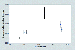
Fig. 1 shows the outcome of one such trial, the determination of ash in animal feeds, a very simple procedure that is unusually precise under reproducibility conditions. It is tempting to assume that there must be an underlying smooth relationship between dispersion and mass fraction, but the statistics show a worrying assortment of outliers/leverage points and clear lack of fit to any sensible function. The mass fractions are poorly spaced. Nevertheless, we must recognise that it would be difficult and expensive for the trial organiser to do better. A fairly obvious interpretation is that a high outlier was probably caused by an atypical test material (molasses, see Fig. 1 caption).
The set of results shown in Fig. 1, however, is not typical of collaborative trials in general: it is in fact better than most outcomes. Firstly, it is an international study, thereby providing a realistic estimate of precision. Secondly, it shows statistics from eight test materials rather than the minimum five, giving more scope for a satisfactory summary of the trend. Even better, each point is determined by no less than about 50 laboratories as opposed to the minimum of eight, so the error bars are about 2.5 times shorter than usual.
Summarising the statistics
Regardless of the shortcomings of the typical collaborative trial, analysts need a statistical summary of the outcome, so that the findings can be applied to practical situations – that is, to infer uncertainties at mass fractions unrepresented in the study. However, it is difficult to see a priori how best to summarise such a miscellany of outcomes, or even whether the attempt is meaningful.Consider the possible options for summarizing the statistics in Fig. 1. Some of these are mentioned in ISO 5725.
(1) A mean relative standard deviation (RSD) (the equivalent of an ordinary least squares regression through the origin), or a robustified version such as the median RSD.
(2) An ordinary least squares regression with an intercept.
(3) A weighted least squares regression with an intercept.
(4) A robust regression with an intercept.
(5) The Horwitz function, viz., σ = 0.02c0.8495 relating standard deviation (σ) with mass fraction c.
(6) A power-law generalization of the Horwitz function, σ = θ1cθ2, with estimated parameters θ1,θ2.
(7) A Zitter–God equation (see below), ![[small sigma, Greek, circumflex]](https://www.rsc.org/images/entities/i_char_e111.gif) 2 = α2 + (βc)2, with parameters α, β estimated by a robust procedure.
2 = α2 + (βc)2, with parameters α, β estimated by a robust procedure.
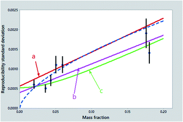
The practical problem in selecting among these possibilities, in a high proportion of collaborative trials, is that the various models are unlikely to be distinguishable as judged by lack-of-fit statistics. Some candidate fits are shown in Fig. 2. Yet statistically we are flummoxed – we cannot guess from the data alone what the best model might be! We can, however, apply the principle of ‘Holmes's Razor’, namely, first eliminate the unsuitable: whatever (if anything) remains must be appropriate. Let's try it!
 | ||
| Fig. 2 Reproducibility standard deviations (points) from the collaborative trial of Fig. 1, with error bars showing 95% confidence intervals. Also shown are: (a) the least squares regression line (red); (b) a robust regression line (violet); (c) the Zitter–God fit (green); and the power-law function (type no. 6 above) (dashed) (point treated as an outlier not shown). | ||
If we are interested in precision at mass fractions approaching a detection limit (often an important consideration), any function implying a zero intercept (items 1, 5 and 6 above) cannot be used: the idea of detection limit implies a strictly positive intercept. A straight-line regression with an intercept (items 2, 3, 4) could be imposed upon many such datasets but suffers from the possible defect that the model implies the addition of standard deviations, rather than variances. Moreover, as we will quite likely encounter gross outliers, or at least significant lack of fit in some of the points, naïve least squares procedures (items 2, 3) could give a biased summary. More crucially, it could provide in some instances an unrealistically small or even negative intercept. Only a robustified fit to a Zitter–God equation (item 7) remains generally applicable.1
Zitter and God proposed their equation in a short paper that seems to have been the first to explore the dependence of standard deviation on mass fraction or concentration but the topic was not followed up by the original authors. Since then it has been tested experimentally and shown to represent rather well precision information obtained at different mass fractions, under various conditions of measurement and in a diverse range of analytical application sectors. It has several attractive features, namely:
• It uses a correct model for the combination of independent uncertainty terms (α2, (βc)2), namely the addition of variances rather than standard deviations.
• It usually provides a positive intercept estimate (![[small alpha, Greek, circumflex]](https://www.rsc.org/images/entities/i_char_e101.gif) ) that is related to the conventional detection limit of about 3.5α.
) that is related to the conventional detection limit of about 3.5α.
• The β parameter is the familiar asymptotic relative standard deviation.
• Both parameters can be estimated easily by a robustified procedure.
Conclusions
Collaborative trials are traditionally taken as unsurpassed for studying the uncertainty of analytical procedures but, whatever their capabilities, they are falling into disuse because of the high costs involved. Current practice in uncertainty estimation is focused on ‘single laboratory validation’ in which several uncertainty terms derivable within-laboratory are combined.However, a third possibility is now available, namely the use of reproducibility standard deviations derived from proficiency tests. Proficiency tests are now almost universal in chemical analysis because of the requirements of accreditation. Over time, so far as we can tell from currently available evidence in food analysis, they provide much the same information as collaborative trials.2 Additionally, they are well-described by the Zitter–God equation.
This Technical Brief was prepared for the Statistics Expert Working Group by Michael Thompson (Birkbeck University of London) and approved by the AMC on 8 November 2021.
Notes and further reading
• Strictly, the reproducibility variance is an unbiased estimate of the square of the standard uncertainty. Taking square roots leaves the standard deviation biased low to the extent of about 0.95 with results from eight participant laboratories. The bias is smaller with a greater participation.• Information about collaborative trials can be found in: W. Horwitz, Protocol for the design, conduct and interpretation of method-performance studies, Pure Appl. Chem., 1995, 67, 331–343.
• A review of the Zitter–God equation shows its wide applicability in chemical measurement. M. Thompson, Uncertainty functions, a compact way of summarising or specifying the behaviour of analytical systems, TrAC Trends Anal. Chem., 2011, 30, 1168–1175.
• ISO 5725-2:2019 provides an explicit fitting method for all of its models, including the Zitter–God equation. The methods given take some account of the uncertainties in both variables.
1. H. Zitter and C. God, Ermittlung, Auswertung und Ursachen von Fehlern bei Betriebsanalysen, Fresenius' Z. Anal. Chem., 1971, 255, 1–9.
2. M. Thompson, M. Sykes, K. Mathieson and R. Wood, Comparison of reproducibility precision on mass fraction in some interlaboratory studies of methods of food analysis, Anal. Bioanal. Chem., October 2021, DOI: 10.1007/s00216-021-03736-3.
| This journal is © The Royal Society of Chemistry 2022 |


