 Open Access Article
Across different instruments about tobacco quantitative analysis model of NIR spectroscopy based on transfer learning
Huanchao Shenab,
Yingrui Genga,
Hongfei Niab,
Hui Wangc,
Jizhong Wuc,
Xianwei Haoc,
Jinxin Tiec,
Yingjie Luoa,
Tengfei Xua,
Yong Chena and
Xuesong Liu *a
*a
aCollege of Pharmaceutical Sciences, Zhejiang University, Hangzhou, 310058, China. E-mail: liuxuesong@zju.edu.cn
bInnovation Institute for Artificial Intelligence in Medicine of Zhejiang University, Hangzhou, 310018, China
cTechnology Center, China Tobacco Zhejiang Industrial Co., Ltd, Hangzhou, 310008, China
First published on 14th November 2022
Abstract
With the development of near-infrared (NIR) spectroscopy, various calibration transfer algorithms have been proposed, but such algorithms are often based on the same distribution of samples. In machine learning, calibration transfer between types of samples can be achieved using transfer learning and does not need many samples. This paper proposed an instance transfer learning algorithm based on boosted weighted extreme learning machine (weighted ELM) to construct NIR quantitative analysis models based on different instruments for tobacco in practical production. The support vector machine (SVM), weighted ELM, and weighted ELM-AdaBoost models were compared after the spectral data were preprocessed by standard normal variate (SNV) and principal component analysis (PCA), and then the weighted ELM-TrAdaBoost model was built using data from the other domain to realize the transfer from different source domains to the target domain. The coefficient of determination of prediction (R2) of the weighted ELM-TrAdaBoost model of four target components (nicotine, Cl, K, and total nitrogen) reached 0.9426, 0.8147, 0.7548, and 0.6980. The results demonstrated the superiority of ensemble learning and the source domain samples for model construction, improving the models' generalization ability and prediction performance. This is not a bad approach when modeling with small sample sizes and has the advantage of fast learning.
1. Introduction
Tobacco is a complex natural product, and the determination of its key chemical indicator content helps control tobacco quality. Nicotine is the most important indicator component in tobacco and has a direct impact on sensory comfort. The levels of both Cl and K affect the combustibility of tobacco. Nitrogen is a key element in tobacco yield, and increasing the accumulation of nitrogenous compounds in the tobacco leaf will result in better-quality tobacco. The chemical analysis of these flavor substance bases is very important in tobacco quality control.NIR spectroscopy is already extensively used in petroleum,1 agriculture,2 chemical,3 tobacco,4 food,5,6 and pharmaceutical7,8 industries since it is a simple, rapid, non-destructive, and reliable analytical method. However, due to the variability of measurement conditions (e.g., change of environmental temperature, and humidity) and instruments (even from the same manufacturer), the calibration models established are often not applicable to new samples or do not provide reliable predictive power. Recalibration can be employed to tackle this tricky problem. However, it requires scans of numerous samples, which is both time-consuming and costly.9 In these circumstances, calibration transfer can be a sensible option to reduce the consumption of recalibration.
A great number of methods have been proposed for calibration transfer, which can be divided into two main types depending on whether standard samples are needed, as shown in Table 1. Classic methods of calibration transfer with standard samples have been proposed. Osborne10 first presented the slope/bias (S/B) algorithm, then Bouveresse11 modified the S/B algorithm and proposed the slope/bias correction (SBC) algorithm. Shenk12 achieved the transfer of the spectral model between different instruments using Shenk's calibration transfer algorithm. Wang13 proposed the Direct Standardization (DS) algorithm which realized full spectral calibration by a transfer matrix. These methods often achieve transfer by applying the model built by the master instrument to the slave instrument. In reality, it is often difficult to obtain standard spectra from master and slave instruments that correspond to each other. Therefore, it is necessary to develop methods without standard samples. Calibration transfer methods without standard samples fall into two main groups: (1) the first group contains preprocessing methods: scatter-correction methods and spectral derivatives.14 The former includes multiplicative scatter correction (MSC), standard normal variate (SNV), etc. The latter can be used to eliminate baseline offsets and linearly sloped baselines (scattering), for example, by taking first- and second-order derivatives.15 However, it is difficult to eliminate spectral differences by relying on preprocessing methods alone. (2) The second group consists mainly of many projection methods, which can subtract the already explained or irrelevant information, such as transfer component analysis (TCA)16 and dynamic orthogonal projection (DOP).17 TCA is completely unsupervised, but TCA assumes that the datasets of the two batches are similar. If the two batches have different output value distributions, this will reduce the performance of TCA. DOP requires a small number of additional measurements to design the impact factor subspace for orthogonal projection against changes in the measuring conditions that induce variations of unknown interfering factors.
| Whether standard samples are needed | Type of method | Example | Characteristics |
|---|---|---|---|
| Standardization | Standardization of the predicted values | S/B, SBC18 | They target the between-instrument variation directly and therefore work more effectively, especially when the instrument difference is large. However, the standard samples must be very stable over the scan period of each instrument involved, and this is difficult20 |
| Standardization of the spectral responses | DS,19 Shenk's algorithm | ||
| Non-standardization | Preprocessing | MSC, SNV, first- and second-order derivatives | They are designed to eliminate specific noise but are less effective for unknown variations |
| Projection | TCA, DOP | They do not require standard samples and look for solutions with the help of a subspace |
The field of machine learning has made significant progress in the last decade. Ensemble learning methods are a class of advanced machine learning methods that train multiple learners and combine them to solve a problem with great success in practice, typically represented by bagging and boosting.21 An ensemble of numerous learners is usually more accurate than a single learner, and the ensemble learning methods show satisfactory performance in many practical tasks.22 Transfer learning has recently emerged to address the problem of how quickly a learning system can adapt to new scenarios, tasks, and environments, aiming to use the knowledge gained in solving one task and apply it to a different but somewhat relevant task.23 Recent studies have reported the employment of transfer learning in spectral data.24,25 TrAdaBoost is an inductive ensemble learning method based on the boosting algorithm, i.e., finding the misleading source domain samples by iteratively updating the source domain sample weights, incorporating the advantages of ensemble learning and transfer learning. Based on the above advantages, the SNV-PCA-weighted ELM-TrAdaBoost method was proposed for the transfer between samples scanned by different instruments. This algorithm attempts to update the weight of each sample in the target and source domain of the training set using the opposite strategy, relying on if it has a negative or positive contribution in each round of iterations. Compared to other calibration transfer algorithms, the proposed machine learning-based method is easier to use, does not depend on standard samples, and requires less knowledge of NIR spectroscopy, making it more suitable for general use. Unlike other calibration transfer algorithms which are based on a model perspective (standardize the regression coefficients, the spectral responses, or the predicted values by mathematical manipulation), the proposed method is based on the transfer of samples.
The contents of this paper are organized as follows. Section 2 details the tobacco dataset and the fundamentals of the weighted ELM and TrAdaBoost algorithms. Section 3 details the experimental protocols, results, and discussion. The model effects of SVM, weighted ELM, and weighted ELM-AdaBoost were compared by using the target domain dataset to validate the advantages of ensemble learning. Weighted ELM-AdaBoost and weighted ELM-TrAdaBoost models were also constructed to analyze the effects of transfer learning. Finally, conclusions are drawn in Section 4.
2. Materials and methods
2.1 Introduction of tobacco dataset
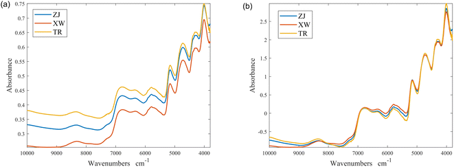
There are eighty-five tobacco samples from 2018 for our experimental design, provided by the Technology Center of the China Tobacco Zhejiang Industrial Co., Ltd. To make samples more representative, different geographical origins were chosen, including Guizhou (14 samples), Hunan (14 samples), Hubei (9 samples), Henan (14 samples), Sichuan (9 samples), and Yunnan (25 samples) provinces. The spectral data of samples were measured in Hangzhou (Zhejiang Province, ZJ), Xuanwei (Yunnan Province, XW), and Tongren (Guizhou Province, TR), using Antaris IIFT-NIR Analyzer (Thermo Fisher Scientific, USA), working with a wavenumber range of 10![[thin space (1/6-em)]](https://www.rsc.org/images/entities/char_2009.gif) 000–3800 cm−1 and a resolution of 8 cm−1. Tobacco powder was placed in a rotating cup over a water-free 50 mm diameter quartz window. Instrument performance was verified before analysis using an instrumental self-test (ValPro System Qualification). Every sample was scanned 72 times and averaged, with each spectrum containing 1609 wavelength points. The values of nicotine, Cl, K, and total nitrogen were measured according to the standards of the tobacco industry of the People's Republic of China YC/T 246-2008, YC/T 162-2011, YC/T 217-2007, and YC/T 161-2002. More details of the tobacco dataset can be seen in Table 2. Data processing and image visualization were done via MATLAB R2020b.
000–3800 cm−1 and a resolution of 8 cm−1. Tobacco powder was placed in a rotating cup over a water-free 50 mm diameter quartz window. Instrument performance was verified before analysis using an instrumental self-test (ValPro System Qualification). Every sample was scanned 72 times and averaged, with each spectrum containing 1609 wavelength points. The values of nicotine, Cl, K, and total nitrogen were measured according to the standards of the tobacco industry of the People's Republic of China YC/T 246-2008, YC/T 162-2011, YC/T 217-2007, and YC/T 161-2002. More details of the tobacco dataset can be seen in Table 2. Data processing and image visualization were done via MATLAB R2020b.
| Component | Minimum value (%) | Maximum value (%) | Mean value (%) | Standard deviation |
|---|---|---|---|---|
| Nicotine | 1.0835 | 3.6220 | 2.5531 | 0.5072 |
| Cl | 0.1910 | 1.1680 | 0.3862 | 0.1782 |
| K | 1.3445 | 3.6190 | 2.0801 | 0.4193 |
| Total nitrogen | 1.6375 | 2.6905 | 2.0293 | 0.2182 |
2.2 Theory and algorithm
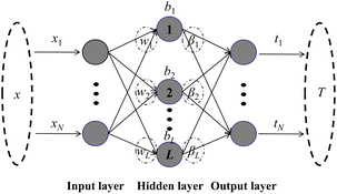
 | (1) |
| Hβ = T | (2) |
| ||Hβ − T ||= 0 | (3) |
 | (4) |
In this paper, the calibration model was built by the weighted ELM method, taking into account that each sample in the training set contributes differently to the model. Weighted ELM28 has recently been proposed to handle data with unbalanced distributions while preserving the strengths of the original ELM. Each sample in the training set is assigned an additional weight. Mathematically, an N × N diagonal matrix W is defined that is related to each training sample xi. The weight matrix
| W = diag(Wii), i = 1, …, N | (5) |
| Weighting strategy 1: Wii = 1/N | (6) |
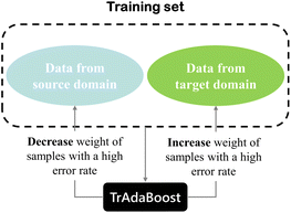
TrAdaBoost, proposed by Dai,30 is an instance-based transfer learning method that enables cross-domain transfer and is a variant of AdaBoost. The TrAdaBoost algorithm is proposed with the idea that some inherent information present in the source domain could be useful for the model construction when building a calibration model of the target domain. In contrast, some of the information in the source domain could be of no use, or even detrimental. TrAdaBoost allows the use of a small amount of newly labeled data combined with old data to generate a high-quality model for the new data, even if the new data is not sufficient to train the model directly, achieving knowledge from old data to new data efficiently. Thus, the TrAdaBoost algorithm attempts to renew the importance of training set samples by giving each sample a different weight. A simple principle for updating the sample weights of the training set of the TrAdaBoost algorithm is shown in Fig. 2. For those samples in the training set that belong to the target domain, the same weight updating strategy is adopted as for the AdaBoost algorithm, while an opposite strategy is used for the samples in the training set that belong to the source domain, samples with higher error rates will receive smaller distribution weights.
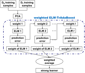
Fig. 3 demonstrates the procedure of the proposed algorithm, which incorporates SNV, PCA, weighted ELM, and the TrAdaBoost algorithm. The spectra are preprocessed with SNV to eliminate scattering at first. Secondly, some samples from the source and target domains are randomly selected to form the training set. Thirdly, PCA is used to extract the low-dimensional features of the high-dimensional spectra. Finally, several quantitative analysis models for calibration transfer have been developed by applying the weighted ELM-TrAdaBoost algorithm, thus constituting a strong learning model. As for the model prediction stage, every sample from the testing set is used as input to each sub-model and the corresponding predicted values are calculated using a weighted average strategy as the final model output.
The detailed steps of the model training phase of the proposed calibration transfer algorithm are as follows:
Input: samples from the source domain {XSi,YSi} (i = 1, …, m); samples from the target domain {XTi,YTi} (i = 1, …, n).
Step 1: the combination of samples from the source and target domains forms the training set {Xk,Yk} (k = 1, …, m + n).
Step 2: taking PCA on Xk (k = 1, …, m + n), calculate the principal component score matrix S, the number of principal components (PCs) Z is then determined based on the cumulative contribution of principal components.
Step 3: initial parameter setting.
| Initial weights for samples from the source domain: wSi = 1/m (i = 1, …, m) | (7) |
| Initial weights for samples from the target domain: wTj = 1/n (j = m + 1, …, m + n) | (8) |
Initial weights for the training set samples: wk = {wSi; wTj} (i = 1, …, m; j = m + 1, …, m + n).
Initial value of the number of iterations: M = 1.
The maximum value of the number of iterations: I = 200 (can be adjusted as appropriate).
The activation function of the weighted ELM is sigmoid.
The number of hidden neurons is 30 (can be adjusted as appropriate).
 | (9) |
Step 4: develop a quantitative analysis model (weak learner) for weighted ELM-based. The input of the model is the first Z PCs SZ (the first Z columns of S).
Step 5: compute the prediction error.
The true value of the training set is Yk (k = 1, …, m + n).
The prediction value of the training set is Pk (k = 1, …, m + n).
Compute the prediction error Ek (k = 1, …, m + n) according to the following equations:
 | (10) |
Step 6: the individual weights and iteration values are updated by the following formulas:
 | (11) |
 | (12) |
| wSi = wSi·βMEi (i = 1, …, m) | (13) |
| wTj = wTj·βM−Ej (j = m + 1, …, m + n) | (14) |
| M = M + 1 | (15) |
Step 7: while M ≤ I, go back step 4; otherwise stop.
Output: the ensemble quantitative analysis model (a series of quantitative analysis models).
2.3 Model evaluation
In this experiment, the performance of the model was assessed by the coefficient of determination of prediction (R2) and root mean square error of prediction (RMSEP), calculated as follows:
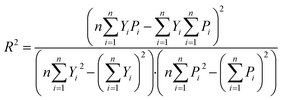 | (16) |
 | (17) |
In general, the smaller the RMSEP, the smaller the prediction error, indicating that the model is more capable of predicting. R2 reflects the generalization ability of the model. R2 is closer to 1, indicating that the generalization ability of the model is better.
3. Experimental design and results
3.1 Spectral data preprocessing
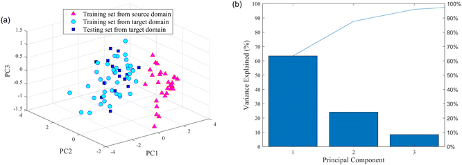 | ||
| Fig. 5 Results of PCA: (a) PC1 vs. PC2 vs. PC3 of the source and target domain; (b) contribution rate of the principal component. | ||
The number of PCs was also selected using the above experimental scheme. The contribution of the first principal component (PC1) was 63.46%, the second principal component (PC2) was 24.15%, and the third principal component (PC3) was 8.39%. Aiming to include as much useful information as possible in the original spectral data, the number of PCs was set to 20, which has a cumulative contribution of 99.99%.
3.2 Experimental protocols
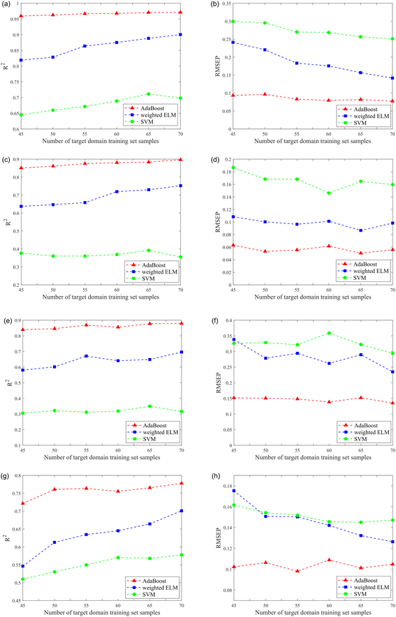
Quantitative analysis models were developed for four components (nicotine, Cl, K, and total nitrogen). From a total of 85 samples, 15 samples were randomly selected from the target domain as the testing set, and 45–70 (5 intervals) samples were randomly selected from the target domain as the training set. All results were average values of 200 runs, overcoming the impact of the model's stochastic parameters. In addition, these models' generalization performance and predictive ability were evaluated by R2 of the testing set and RMSEP. The results are shown in Fig. 6, and more details can be seen in Table 3.
| Component | Model | Number of target domain training set samples | ||||||
|---|---|---|---|---|---|---|---|---|
| 45 | 50 | 55 | 60 | 65 | 70 | |||
| a AdaBoost represents weighted ELM-AdaBoost. | ||||||||
| Nicotine | SVM | R2 | 0.6451 | 0.6597 | 0.6716 | 0.6890 | 0.7115 | 0.6984 |
| RMSEP | 0.2996 | 0.2954 | 0.2701 | 0.2686 | 0.2567 | 0.2512 | ||
| Weighted ELM | R2 | 0.8190 | 0.8285 | 0.8639 | 0.8752 | 0.8884 | 0.9006 | |
| RMSEP | 0.2413 | 0.2206 | 0.1833 | 0.1757 | 0.1568 | 0.1418 | ||
| AdaBoosta | R2 | 0.9596 | 0.9627 | 0.9669 | 0.9678 | 0.9707 | 0.9713 | |
| RMSEP | 0.0935 | 0.0965 | 0.0830 | 0.0795 | 0.0819 | 0.0776 | ||
| Cl | SVM | R2 | 0.3764 | 0.3602 | 0.3603 | 0.3691 | 0.3920 | 0.3551 |
| RMSEP | 0.1867 | 0.1682 | 0.1682 | 0.1460 | 0.1647 | 0.1594 | ||
| Weighted ELM | R2 | 0.6372 | 0.6466 | 0.6583 | 0.7192 | 0.7299 | 0.7524 | |
| RMSEP | 0.1084 | 0.1003 | 0.0964 | 0.1012 | 0.0866 | 0.0983 | ||
| AdaBoost | R2 | 0.8506 | 0.8611 | 0.8754 | 0.8804 | 0.8835 | 0.8967 | |
| RMSEP | 0.0631 | 0.0532 | 0.0555 | 0.0616 | 0.0504 | 0.0558 | ||
| K | SVM | R2 | 0.3054 | 0.3221 | 0.3117 | 0.3190 | 0.3496 | 0.3165 |
| RMSEP | 0.3261 | 0.3285 | 0.3214 | 0.3588 | 0.3224 | 0.2940 | ||
| Weighted ELM | R2 | 0.5811 | 0.6017 | 0.6708 | 0.6410 | 0.6490 | 0.6963 | |
| RMSEP | 0.3382 | 0.2785 | 0.2942 | 0.2619 | 0.2897 | 0.2349 | ||
| AdaBoost | R2 | 0.8393 | 0.8458 | 0.8687 | 0.8554 | 0.8776 | 0.8792 | |
| RMSEP | 0.1517 | 0.1506 | 0.1482 | 0.1384 | 0.1520 | 0.1350 | ||
| Total nitrogen | SVM | R2 | 0.5101 | 0.5302 | 0.5496 | 0.5703 | 0.5678 | 0.5777 |
| RMSEP | 0.1616 | 0.1542 | 0.1518 | 0.1456 | 0.1451 | 0.1471 | ||
| Weighted ELM | R2 | 0.5463 | 0.6128 | 0.6346 | 0.6452 | 0.6643 | 0.7011 | |
| RMSEP | 0.1753 | 0.1507 | 0.1503 | 0.1421 | 0.1323 | 0.1264 | ||
| AdaBoost | R2 | 0.7216 | 0.7608 | 0.7636 | 0.7553 | 0.7655 | 0.7780 | |
| RMSEP | 0.1023 | 0.1064 | 0.0981 | 0.1089 | 0.1012 | 0.1048 | ||
The superiority of the ensemble learning approach is demonstrated by the fact that the generalization performance and predictive ability of the quantitative analysis model can be greatly improved by performing ensemble learning on each component. Taking the results of ensemble learning for nicotine (Fig. 6(a) and (b)) as an example, the results showed that although the training set contained only 45 samples, the R2 of the testing set after ensemble learning could reach 0.9596. In comparison, if a model based on weighted ELM was built directly, the corresponding R2 was only 0.8190. The performance of the weighted ELM and weighted ELM-AdaBoost were better than SVM. Moreover, as the number of samples in the training set increased, the R2 tended to increase gradually, while the RMSEP tended to decrease gradually. When the number of samples in the training set of the target domain was 70, the R2 of weighted ELM-AdaBoost reached 0.9713 and the RMSEP was only 0.0776. Similarly, the results for the other three components showed the same trend.
| Source domain | Component | Method | Number of target domain training set samples | |||||
|---|---|---|---|---|---|---|---|---|
| 30 | 31 | 32 | 33 | 34 | 35 | |||
| a TrAdaBoost represents weighted ELM-TrAdaBoost.b AdaBoost represents weighted ELM-AdaBoost. | ||||||||
| XW | Nicotine | TrAdaBoosta | 0.5650 | 0.8877 | 0.9293 | 0.9400 | 0.9372 | 0.9426 |
| AdaBoostb | 0.3272 | 0.8597 | 0.9134 | 0.9285 | 0.9328 | 0.9374 | ||
| Cl | TrAdaBoost | 0.5827 | 0.7082 | 0.7579 | 0.7775 | 0.7835 | 0.8147 | |
| AdaBoost | 0.2349 | 0.5970 | 0.7258 | 0.7380 | 0.7672 | 0.7917 | ||
| K | TrAdaBoost | 0.2876 | 0.6421 | 0.6871 | 0.7494 | 0.7713 | 0.7548 | |
| AdaBoost | 0.2163 | 0.6174 | 0.6612 | 0.7263 | 0.7518 | 0.7502 | ||
| Total nitrogen | TrAdaBoost | 0.4298 | 0.6310 | 0.6550 | 0.6632 | 0.6705 | 0.6980 | |
| AdaBoost | 0.1666 | 0.5640 | 0.5943 | 0.6205 | 0.6445 | 0.6808 | ||
| TR | Nicotine | TrAdaBoost | 0.6257 | 0.8595 | 0.9194 | 0.9378 | 0.9358 | 0.9432 |
| AdaBoost | 0.2946 | 0.7947 | 0.9009 | 0.9274 | 0.9300 | 0.9341 | ||
| Cl | TrAdaBoost | 0.7096 | 0.7585 | 0.7906 | 0.8076 | 0.8094 | 0.8228 | |
| AdaBoost | 0.2506 | 0.6279 | 0.7386 | 0.7841 | 0.7858 | 0.8040 | ||
| K | TrAdaBoost | 0.3350 | 0.6156 | 0.7352 | 0.7573 | 0.7731 | 0.8045 | |
| AdaBoost | 0.2016 | 0.5755 | 0.7113 | 0.7516 | 0.7564 | 0.7953 | ||
| Total nitrogen | TrAdaBoost | 0.5205 | 0.6115 | 0.6266 | 0.6691 | 0.6662 | 0.6960 | |
| AdaBoost | 0.1896 | 0.5170 | 0.5757 | 0.6272 | 0.6311 | 0.6723 | ||
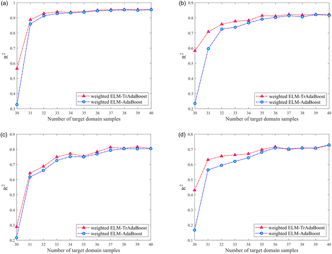
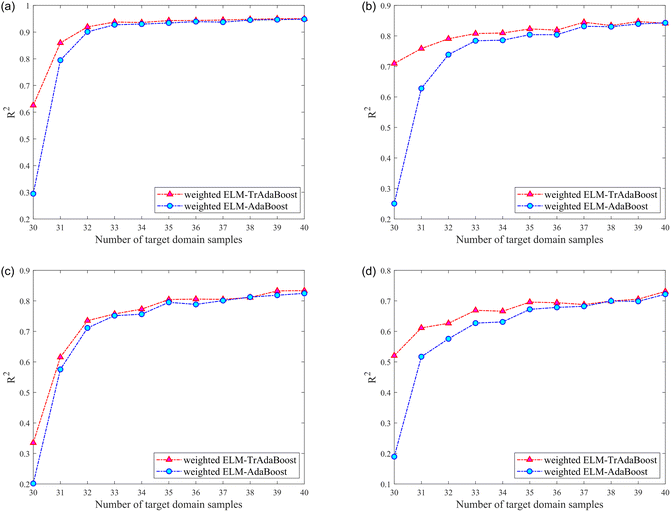
It can be noticed that the R2 of the testing set was higher than that of the model without calibration transfer after the calibration transfer of the four components from different instruments (source domains). The improvement in model performance with calibration transfer was more pronounced when the number of samples in the training set of the target domain was small, and this advantage gradually diminishes as the number of samples increases. However, the general result was still better for calibration transfer than without. Regarding the gradual weakening of the advantage of transfer learning, reasonably, as the number of samples from the target domain involved in the training set of the model gradually increases, the role of samples from the source domain in the model gradually diminishes.
3.3 Discussion
In the field of machine learning, the computational effort of the model deserves to be discussed. The proposed method is based on weighted ELM, which is simple in structure and fast in computation, in addition, the input spectral data undergoes a PCA dimensionality reduction from 1609 to 20 dimensions, which also improves the execution speed of the algorithm. The proposed method (weighted ELM-TrAdaBoost) has a model training time of approximately 0.04 seconds for one run, confirming the small computational cost.It is commonly assumed that more samples usually lead to better model performance. Meanwhile, more samples also bring an increased computational burden. Thus, a trade-off between the number of samples and the computational burden is necessary. Here, experimental protocol #2 (XW to ZJ, component: nicotine) was taken as an example of the following discussion.
Fig. 9 demonstrates the effect of the variation in the number of source domain samples on the performance of the quantitative analysis model. It can be found that increasing the number of samples in the source domain of the training set will remarkably increase the R2 of the calibration transfer model when the training set contains relatively few samples in the target domain (Fig. 9(a) and (b)). However, when the number of samples in the target domain of the training set increased, the increase in the number of samples in the source domain did not obviously improve the R2 of the calibration model (Fig. 9(d)–(f)). Since when the training set contains enough target domain samples, setting up a quantitative analysis model with excellent generalization power is a simple matter, so the information that can be provided by the source domain sample appears insignificant. Conversely, when the training set contained fewer target domain samples, the information contained in the source domain samples helped build the target domain model, despite the instruments in the source and target domains being different.
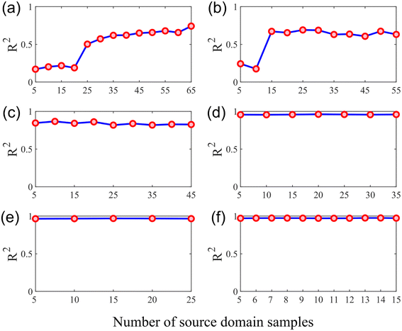 | ||
| Fig. 9 Effects of the number of source domain samples on the R2 of the model: (a) the number of target domain samples is 10 (N = 10); (b) N = 20; (c) N = 30; (d) N = 40; (e) N = 50; (f) N = 60. | ||
4. Conclusions
Many of the existing calibration transfer methods have limited application as they are based on standard samples, the preservation of which is a challenge. When environmental conditions, instruments, or sample changes occur, the original model is no longer applicable, while the method proposed avoids the drawback of rescanning a large number of samples for modeling. In this paper, a novel instance-based method for calibration transfer is applied to tobacco quality evaluation across different instrumentation domains, which incorporates SNV, PCA, weighted ELM, and TrAdaBoost algorithms. The results suggested that the proposed method could achieve calibration transfer between different instruments. In existing studies, the transfer from one source domain to one target domain has been realized with promising performance. The R2 of the TrAdaBoost model of four components (nicotine, Cl, K, and total nitrogen) of tobacco reached 0.9426, 0.8147, 0.7548, and 0.6980 (transfer from XW to ZJ as an example). In reality, production data often involves the distribution of multiple domains, so it is a question worth investigating whether the information from multiple source domains can be transferred to the target domain. The proposed method should be tried out for more than just cross-instrument transfers, such as with different sample states, different compositions, etc.Author contributions
Huanchao Shen, methodology, data analysis, visualization, writing-original draft. Yingrui Geng, conceptualization, writing-reviewing and editing. Hongfei Ni, conceptualization, writing-reviewing and editing. Hui Wang, data provision. Jizhong Wu, data provision. Xianwei Hao, data provision. Jinxin Tie, data provision. Yingjie Luo, writing-reviewing and editing. Tengfei Xu, writing-reviewing and editing. Yong Chen, writing-reviewing and editing. Xuesong Liu, conceptualization, writing-reviewing and editing, supervision, funding acquisition.Conflicts of interest
There are no conflicts to declare.Acknowledgements
The authors would like to acknowledge that this work was partially supported by the Science Foundation of China Tobacco Zhejiang Industrial (grant no. ZJZY2021A020, grant no. ZJZY2021A001).References
- F. D. Santos, S. G. T. Vianna, P. H. P. Cunha, G. S. Folli, E. H. de Paulo, M. K. Moro, W. Romão, E. C. de Oliveira and P. R. Filgueiras, Microchem. J., 2022, 181, 107696 CrossRef CAS.
- L. Li, X. Jang, B. Li and Y. Liu, Comput. Electron. Agric., 2021, 190, 106448 CrossRef.
- O. Daikos, M. Naumann, K. Ohndorf, C. Bundesmann, U. Helmstedt and T. Scherzer, Talanta, 2021, 223, 121696 CrossRef CAS PubMed.
- B. Xiang, C. Cheng, J. Xia, L. Tang, J. Mu and Y. Bi, Vib. Spectrosc., 2020, 111, 103182 CrossRef CAS.
- S. S. Nallan Chakravartula, R. Moscetti, G. Bedini, M. Nardella and R. Massantini, Food Control, 2022, 135, 108816 CrossRef CAS.
- S. Chang, C. Yin, S. Liang, M. Lu, P. Wang and Z. Li, Anal. Methods, 2020, 12, 2469–2475 RSC.
- S. Assi, B. Arafat, K. Lawson-Wood and I. Robertson, Appl. Spectrosc., 2021, 75, 434–444 CrossRef CAS PubMed.
- Q. Xie, R. Wu, X. Zhong, Y. Dong and Q. Fan, RSC Adv., 2018, 8, 27037–27044 RSC.
- Z. Huang, A. Sanaeifar, Y. Tian, L. Liu, D. Zhang, H. Wang, D. Ye and X. Li, J. Food Eng., 2021, 293, 110374 CrossRef CAS.
- B. G. Osborne and T. Fearn, Int. J. Food Sci. Technol., 1983, 18, 453–460 CrossRef.
- E. Bouveresse, C. Hartmann and D. L. Massart, Anal. Chem., 1996, 68, 982–990 CrossRef CAS.
- J. S. Shenk and M. O. Westerhaus, Optical instrument calibration system, US Pat., 4866644, filed 1986, issued 1989 Search PubMed.
- Y. Wang, D. J. Veltkamp and B. R. Kowalski, Anal. Chem., 1991, 63(23), 2750–2756 CrossRef CAS.
- Å. Rinnan, F. v. d. Berg and S. B. Engelsen, Trends Anal. Chem., 2009, 28, 1201–1222 CrossRef.
- R. N. Feudale, N. A. Woody, H. Tan, A. J. Myles, S. D. Brown and J. Ferré, Chemom. Intell. Lab. Syst., 2002, 64, 181–192 CrossRef CAS.
- S. J. Pan, I. W. Tsang, J. T. Kwok and Q. Yang, IEEE Trans. Neural Netw., 2011, 22, 199–210 Search PubMed.
- P. Mishra, J. M. Roger, D. N. Rutledge and E. Woltering, Postharvest Biol. Technol., 2020, 170, 111326 CrossRef CAS.
- X. Dong, J. Dong, Y. Li, H. Xu and X. Tang, Comput. Electron. Agric., 2019, 156, 669–676 CrossRef.
- B. Zou, X. Jiang, H. Feng, Y. Tu and C. Tao, Sci. Total Environ., 2020, 701, 134890 CrossRef CAS PubMed.
- X. Luo, A. Ikehata, K. Sashida, S. Piao, T. Okura and Y. Terada, J. Near Infrared Spectrosc., 2017, 25, 15–25 CrossRef CAS.
- X. Bian, C. Zhang, X. Tan, M. Dymek, Y. Guo, L. Lin, B. Cheng and X. Hu, Anal. Methods, 2017, 9, 2983–2989 RSC.
- Y. Zhou, Z. Zuo, F. Xu and Y. Wang, Spectrochim. Acta, Part A, 2020, 226, 117619 CrossRef CAS PubMed.
- Y. Yu, J. Huang, S. Liu, J. Zhu and S. Liang, Measurement, 2021, 177, 109340 CrossRef.
- X. Li, Z. Li, X. Yang and Y. He, Comput. Electron. Agric., 2021, 186, 106157 CrossRef.
- Y.-y. Chen and Z.-b. Wang, Chemom. Intell. Lab. Syst., 2019, 192, 103824 CrossRef CAS.
- G.-B. Huang, Q.-Y. Zhu and C.-K. Siew, Neurocomputing, 2006, 70, 489–501 CrossRef.
- K. Li, X. Kong, Z. Lu, L. Wenyin and J. Yin, Neurocomputing, 2014, 128, 15–21 CrossRef.
- W. Zong, G.-B. Huang and Y. Chen, Neurocomputing, 2013, 101, 229–242 CrossRef.
- R. E. Schapire, The boosting approach to machine learning: an overview, in Nonlinear Estimation and Classification, ed. D. D. Denison, M. H. Hansen, C. C. Holmes, B. Mallick and B. Yu, Springer, New York, USA, 2003, pp. 149–171 Search PubMed.
- W. Dai, Q. Yang, G.-R. Xue and Y. Yu, Boosting for transfer learning, in Proceedings of the 24th International Conference on Machine Learning (ICML 07), Association for Computing Machinery, New York, USA, 2007, pp. 193–200 Search PubMed.
- Y. Huang, W. Dong, Y. Chen, X. Wang, W. Luo, B. Zhan, X. Liu and H. Zhang, Chemom. Intell. Lab. Syst., 2021, 210, 104243 CrossRef CAS.
- S. Srivastava and H. N. Mishra, Chemom. Intell. Lab. Syst., 2022, 221, 104489 CrossRef CAS.
| This journal is © The Royal Society of Chemistry 2022 |

