
 Open Access Article
 This Open Access Article is licensed under a Creative Commons Attribution-Non Commercial 3.0 Unported Licence
Conceptual density functional theory under pressure: Part I. XP-PCM method applied to atoms†
J.
Eeckhoudt
 a,
T.
Bettens
a,
P.
Geerlings
a,
R.
Cammi
b,
B.
Chen
cd,
M.
Alonso
a and
F.
De Proft
*a
a,
T.
Bettens
a,
P.
Geerlings
a,
R.
Cammi
b,
B.
Chen
cd,
M.
Alonso
a and
F.
De Proft
*a
aGeneral Chemistry Department (ALGC), Vrije Universiteit Brussel (VUB), Brussels, Belgium. E-mail: fdeprof@vub.be
bDepartment of Chemical Science, Life Science and Environmental Sustainability, University of Parma, Parma, Italy
cDonostia International Physics Center, Donostia-San Sebastian, Spain
dIKERBASQUE, Basque Foundation for Science, Plaza Euskadi 5, 48009 Bilbao, Spain
First published on 15th July 2022
Abstract
High pressure chemistry offers the chemical community a range of possibilities to control chemical reactivity, develop new materials and fine-tune chemical properties. Despite the large changes that extreme pressure brings to the table, the field has mainly been restricted to the effects of volume changes and thermodynamics with less attention devoted to electronic effects at the molecular scale. This paper combines the conceptual DFT framework for analyzing chemical reactivity with the XP-PCM method for simulating pressures in the GPa range. Starting from the new derivatives of the energy with respect to external pressure, an electronic atomic volume and an atomic compressibility are found, comparable to their enthalpy analogues, respectively. The corresponding radii correlate well with major known sets of this quantity. The ionization potential and electron affinity are both found to decrease with pressure using two different methods. For the electronegativity and chemical hardness, a decreasing and increasing trend is obtained, respectively, and an electronic volume-based argument is proposed to rationalize the observed periodic trends. The cube of the softness is found to correlate well with the polarizability, both decreasing under pressure, while the interpretation of the electrophilicity becomes ambiguous at extreme pressures. Regarding the electron density, the radial distribution function shows a clear concentration of the electron density towards the inner region of the atom and periodic trends can be found in the density using the Carbó quantum similarity index and the Kullback–Leibler information deficiency. Overall, the extension of the CDFT framework with pressure yields clear periodic patterns.
1. Introduction
From a physical point of view, pressure is defined as the normal force acting on a surface divided by the surface area. At the microscopic level, pressure arises from the collisions of atoms and molecules with the container of the system. This kinetic definition of pressure is identical to the pressure variable known in thermodynamics and is, together with temperature, one of the forefront external parameters to control chemical reactions.In the 19th century, the research into high pressure chemistry commenced with studies of the compressibility and dilatability of gases.1–3 At ambient conditions, the effects of pressure on chemical reactivity are rather limited to the influence on reaction equilibria and phase transition temperatures. An example of the importance of pressure in controlling reaction equilibria is the famous Haber–Bosch process for ammonia synthesis discovered in 1909.4 As pressure increases further, non-covalent interactions, which are very important for biological systems and in biotechnology, are impacted first.5–9 Apart from the reaction equilibrium, the reaction rate can be controlled depending on the so-called volume of activation.10–13 In the context of organic chemistry, new reaction modes become available, offering increased selectivity and a measure of stereocontrol.10,14–17 Still mostly below 10 GPa, a severe reduction of the volume occurs as the van der Waals space is squeezed out.18–20 At extreme pressures, new crystalline phases of known materials have been discovered, providing access to new materials with extraordinary electrical, magnetic and optical properties.20–22 Generally, bonds strengthen and coordination numbers rise as the pressure increases and each electronic energy level is influenced to a different extent, possibly resulting in a redistribution of electrons over the shell structure.18–20,23 Finally, at the highest currently achievable pressures in a laboratory experiment, metallization is expected to occur for all compounds due to the forced overlap of orbitals (e.g. at approximately 450 GPa for hydrogen) and even the spherical symmetry of atoms can be broken to obtain a more efficient stacking.19,20,24–26
To investigate the extreme pressure regime in the gigapascal range, several techniques have been developed both on the experimental and theoretical level. Already in 1905, the Nobel Laureate in Physics P. W. Bridgeman built the first Bridgeman press, an innovative machine capable of reaching pressures up to 100 GPa.27 A next generation of high pressure devices comprises Diamond Anvil Cells (DACs), which utilize flattened diamond tips to attain even higher pressures.28–30 Finally, shockwave compression technology is mentioned as a technique originating from the aeronautics sector using detonations, kinetic impacts or lasers to generate fast releases of energy and is currently being applied for investigations of reaction kinetics and equations of state.31,32
Apart from these experimental achievements, several theoretical techniques have been developed to model chemistry at extreme pressures at the molecular level, focusing on the influence of pressure on structural and spectroscopic properties. Because pressure cannot be explicitly defined on a single molecule, pressure does not enter the Hamiltonian operator directly and different approaches have been proposed to tackle various aspects of the high pressure effects. While still ongoing, basic confinement models that place atoms and molecules in hard and soft confining potentials were historically the first steps in simulating high pressure conditions.33–35 Next, developments in Molecular Dynamics (MD) simulations allowed the modelling of extended systems under pressure. These simulations employ some type of barostat to maintain the desired pressure throughout the simulation e.g. by changing the system volume.36–39 While this type of simulations is widely applied to investigate systems at high pressure, they are computationally demanding, especially when combined with ab initio calculations. Another series of models to simulate pressure focusses on the geometric effects of external pressure through the application of a force on all nuclei towards the geometric centroid. Examples of these models include the Generalized Force Mediated Potential Energy Surface (G-FMPES) and the Hydrostatic Compression Force Field (HCFF).40,41 Other models applicable to single molecules also exist which do take the compression of the electronic cloud into account. One model places the system of interest inside a helium supercell that is constraint to pressure specific dimensions of a pure helium lattice.42 The Gaussians On Surface Tesserae Simulate Hydrostatic Pressure (GOSTSHYP) model simulates pressure by placing repulsive Gaussian potentials on a molecular surface to generate an inward, compressing force.43 Finally, the eXtreme Pressure Polarizable Continuum Model (XP-PCM), introduced by one of the present authors, confines the system inside a molecular cavity and transfers pressure to the system through a repulsive Pauli potential outside of the cavity.44 This model has been applied to a wide range of chemical problems for molecules under pressure, including the calculation and interpretation of the activation volume in chemical reactions,13,45 the change in vibrational frequencies46,47 and electronic excitations,48 and other electronic properties49 induced by pressure.
This variety of experimental and theoretical techniques has allowed access to new materials exhibiting extreme and tunable properties. A number of NaxCly phases have been found, for example, through the combination of theoretical and DAC experiments50 and a LiHn metal has been predicted at a fraction of the metallization pressure of pure hydrogen.51 Additionally, super hard materials have been identified as available through high pressure synthesis, naming for example certain borides52 and monoclinic carbon.53,54
The field of superconductivity has greatly benefited from the advancements in high pressure chemistry with the identification of a range of metallic hydrides55–58 and hydrogen sulfide59 as superconductors at extreme pressure. Finally, noble gases are mentioned as potential components of stable compounds at high pressure, krypton and xenon taking the lead in this regard, since Bartlett et al. synthesized the first noble gas compounds, including a compound of xenon and hexafluoro platinum, Xe[PtF6]x (1 ≤ x ≤ 2), in 1962.60–62
In the present work, the aforementioned XP-PCM technique is used for extending the conceptual density functional theory (conceptual DFT) framework to include the effect of pressure on atomic systems. Conceptual DFT is a branch of DFT,63 which emerged under the impetus of R. G. Parr at the end of the 1970s,64 with the aim of giving precision to widely used but often vaguely defined quantities used to characterize the electronic properties of atoms and molecules and their role in describing chemical reactivity.65–68 Well known examples are Mulliken's electronegativity69 and Pearson's hardness.70 The basic idea is to formulate these quantities as response functions of the energy E with respect to perturbations in the number of electrons N and/or the external potential v(![[r with combining right harpoon above (vector)]](https://www.rsc.org/images/entities/char_0072_20d1.gif) ), the typical perturbations at stake in a chemical reaction.65–68 Written as partial derivatives of the type
), the typical perturbations at stake in a chemical reaction.65–68 Written as partial derivatives of the type 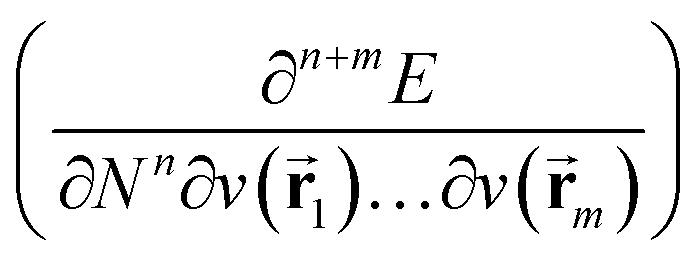 , their global (
![[r with combining right harpoon above (vector)]](https://www.rsc.org/images/entities/b_char_0072_20d1.gif) -independent), local (-dependent) and non-local (1, 2, … dependent) character can be discerned. In recent years, extensions of the functional E = E[N,v], the basic functional considered in the early conceptual DFT years, were at stake with spin,71 temperature,72 external electric,73 magnetic fields,74 and even mechanical forces75,76 and confinement.35,77,78 This endeavor was incited to cope with the ever-increasing diversity in reaction conditions that nowadays can be realized in the laboratory. Pressure, however, has not been explicitly included yet, though confinement can be considered as a forerunner. The present work aims at extending conceptual DFT and exploring the pressure dependence of conceptual DFT quantities such as the Mulliken electronegativity, hardness, electrophilicity and the density itself. The selected test systems are the main group atoms from hydrogen to krypton. In this sense, the present study can be perceived as an extension of the recent work by Rahm et al.79 on the influence of pressure on the Allen scale of electronegativity throughout the periodic table, which is to the best of our knowledge, together with the work of Cammi on the influence of pressure on electron densities44,80 and a very recent paper on electronegativity and hardness under pressure by Dong et al.81 which came out during the review process of the current work, the only study in the field hitherto.
-independent), local (-dependent) and non-local (1, 2, … dependent) character can be discerned. In recent years, extensions of the functional E = E[N,v], the basic functional considered in the early conceptual DFT years, were at stake with spin,71 temperature,72 external electric,73 magnetic fields,74 and even mechanical forces75,76 and confinement.35,77,78 This endeavor was incited to cope with the ever-increasing diversity in reaction conditions that nowadays can be realized in the laboratory. Pressure, however, has not been explicitly included yet, though confinement can be considered as a forerunner. The present work aims at extending conceptual DFT and exploring the pressure dependence of conceptual DFT quantities such as the Mulliken electronegativity, hardness, electrophilicity and the density itself. The selected test systems are the main group atoms from hydrogen to krypton. In this sense, the present study can be perceived as an extension of the recent work by Rahm et al.79 on the influence of pressure on the Allen scale of electronegativity throughout the periodic table, which is to the best of our knowledge, together with the work of Cammi on the influence of pressure on electron densities44,80 and a very recent paper on electronegativity and hardness under pressure by Dong et al.81 which came out during the review process of the current work, the only study in the field hitherto.
The structure of the paper is as follows; first the traditional conceptual DFT is extended to include pressure with the introduction of two new global response functions involving only derivations with respect to pressure  . Next, the response of traditional conceptual DFT global reactivity indices with respect to pressure are examined starting from the ionization potential and the electron affinity, being the basic ingredients in the mathematical definition of the reactivity indices (vide infra). The electronegativity, chemical hardness and electrophilicity are considered, leading to conceptual DFT reactivity descriptors of the mixed type
 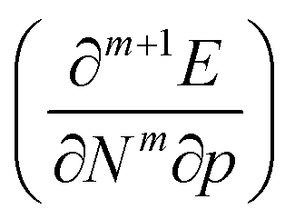 . Finally, the pressure dependence of the first-order local descriptor, the electron density, is investigated by means of the radial distribution function, the Carbó similarity index and the Kullback–Leibler information deficiency.
2. Methodology
2.1 Conceptual density functional theory
In the original formulation of conceptual DFT, the energy E of any electronic system can be expanded according to a Taylor series within its constituting variables N and v() (eqn (1)). The response functions arising in this way are used in the domain of conceptual DFT to rationalize and quantify different aspects of chemical reactivity.67 | (1) |
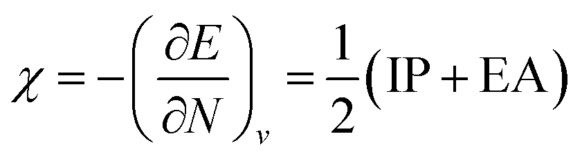
One of the oldest reactivity descriptors is the electronegativity, for which Pauling's definition proposed in 1932 was dominant for decades.82 This quantity can be retrieved in conceptual DFT as the negative of the first-order derivative of the energy with respect to the number of electrons N, resulting in an expression analogous to Mulliken's definition of the electronegativity69χ, widely used today (eqn (2)). The exact nature of the relationship between the energy E and the number of electrons N is a series of straight lines which are interconnected at integer values of N.83 This results in the existence of two one-sided derivatives at N = N0, being equal to the negative of the ionization potential and the electron affinity for the left- and right-handed derivatives  and
and  , respectively. However, when a quadratic function is used to model E(N), the derivative can be found according to the formula in eqn (2), bearing a striking resemblance to the Mulliken scale for electronegativity.64
 | (2) |
 | (3) |
A different scheme for a Taylor expansion considers the grand canonical potential Ω[μ,v] rather than the energy functional. Instead of the hardness, one finds the softness S as the second-order global derivative in casu with respect to the chemical potential.85 This quantity is equal to the inverse of the hardness at a temperature of zero Kelvin and carries similar information as the hardness. Additionally, its cube has been empirically correlated to the polarizability α of the system.86–91 A final global descriptor of chemical reactivity derived from conceptual DFT response functions is the electrophilicity index ω.92,93 This quantity denotes the ability of a system to accept charge when immersed into an infinite, idealized, zero temperature free electron sea. The resulting energy stabilization is the electrophilicity index, given in eqn (4).
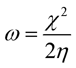 | (4) |
As mentioned above, in recent years, additional variables have been introduced in the E[N,v] functional. These new variables (e.g. electric field, magnetic field) lead to additional terms in the Taylor expansion (eqn (1)) of the form  , involving new response functions. In the case of pressure its influence on the energy and the conventional DFT descriptors χ, η, … gives rise to phenomenological coefficients, new response functions providing valuable information on the change in reactivity when the pressure is altered.
Contrary to the derivatives with respect to the number of electrons only, derivatives with respect to the external potential v() and related mixed derivatives are dependent on and are thus local descriptors. Using a perturbational approach, the first derivative of the energy with respect to v() can be shown to be equal to the electron density ρ() itself.65–67 This density is not only the core variable in DFT, but is a key ingredient in analyzing chemical reactivity and its dependence on the external pressure will be discussed herein. Since this descriptor retains three variables due to its spatial dependence, a number of schemes can be applied to further condense this information. The Radial Distribution Function (RDF), for example, provides the evolution of the density as a function of the distance from a reference point (e.g. the nucleus in the case of atoms) and can be obtained using eqn (5).
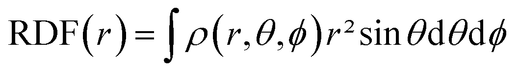 | (5) |
To further condense this information and transition to a quantitative analysis, specific indices to compare electron densities can be applied. In the 1980s, Carbó et al. suggested a general approach for quantifying the so-called quantum similarity between two distributions.94 From this approach, a simple expression for comparing the distributions of two systems, here electron densities, can be obtained, resulting in an overlap-like Quantum Similarity Measure (QSM) (eqn (6)). To normalize this result, eqn (7) can be used, resulting in the quantum similarity index (QSI), quantifying the similarity between two distributions A and B, comprised between 0 and 1.
 | (6) |
 | (7) |
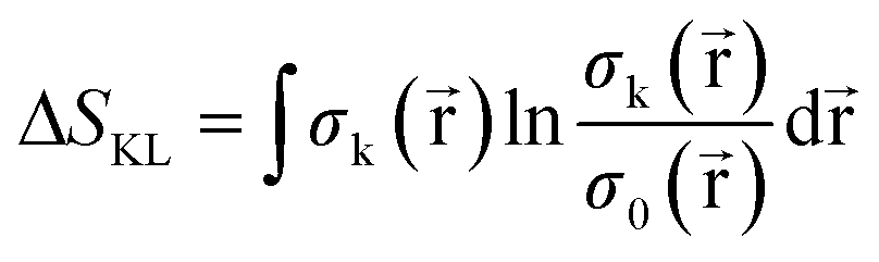
Since this index is known to be rather unsensitive to small changes between distributions,95 a different measure from information theory that characterizes the dissimilarity between two distributions, known as the Kullback–Leibler Information Deficiency ΔSKL, was also used in our analysis.96 This approach fits the ever-increasing importance of Information Theory in Conceptual DFT.68 Generally, this measure is considered the most unbiased way to compare the information contained in two distributions96 and is given by eqn (8), where σ() is the shape function,97 equal to ρ()/N, and the natural logarithm is the ‘surprisal’ yielding the discrimination power between the system k and the reference system 0.98
 | (8) |
2.2 Extreme pressure – polarizable continuum model
To simulate the extreme pressures that are of interest in this paper, the XP-PCM method, originally devised by Cammi et al., is utilized.44,99 This method extends the polarizable continuum model (PCM) to a wide range of pressures by invoking the thermodynamic relationship between energy and pressure and implementing some empirical relationships concerning equations of state. In the traditional PCM model, a solute system is immersed in a void, molecular cavity constructed from a series of nucleus-centered atomic spheres within a dielectric medium characterized by a relative dielectric permittivity ε0 and number density n0S. Due to the charge distribution of the solute, the medium is polarized leading to a range of attractive and repulsive interactions, which are represented by additional non-linear terms within the electronic Hamiltonian in eqn (9).100[Ĥelec + ![[V with combining circumflex]](https://www.rsc.org/images/entities/i_char_0056_0302.gif) e(Ψi) + r]Ψi = EΨi e(Ψi) + r]Ψi = EΨi | (9) |
One of these interactions, the Pauli repulsion r, arises from the forced overlap of the electron density of the solute and the polarizable medium and gives rise to a constant potential barrier Z0 outside of the molecular cavity. The repulsion energy is subsequently calculated according to eqn (10), where ![[small rho, Greek, circumflex]](https://www.rsc.org/images/entities/i_char_e0b7.gif) () is the electron density operator and Θ() is a Heaviside function that is equal to one outside and zero inside of the cavity.
() is the electron density operator and Θ() is a Heaviside function that is equal to one outside and zero inside of the cavity.
 | (10) |
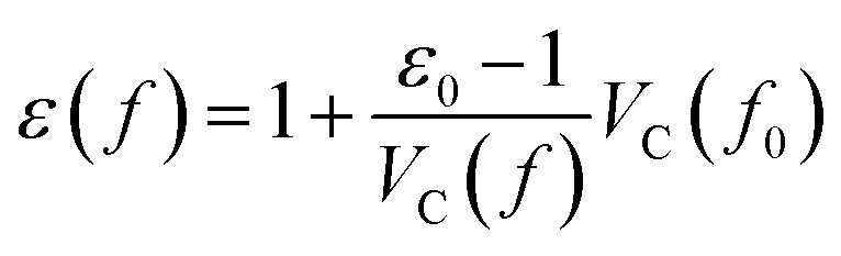
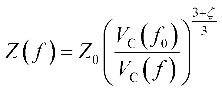
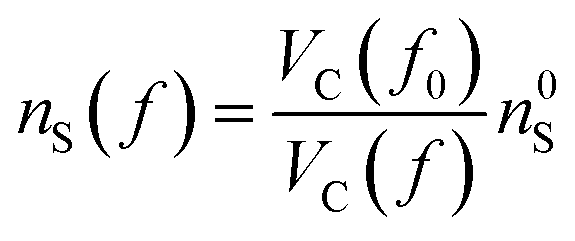
Starting from the reference conditions of PCM calculations, an increased pressure can be achieved by gradually compressing the molecular cavity VC through a decrease of the radii of the spheres comprising the cavity. This is achieved by reducing the scaling factor f that is multiplied with a set of van der Waals radii to obtain the cavity radii, starting from the reference value f0 at standard conditions for that specific set. In addition to the contraction of the cavity, the surrounding dielectric medium is modified through the relative dielectric constant, number density and Pauli barrier according to eqn (11)–(13), where ε0, n0S and Z0 are standard values in PCM for the relative dielectric constant, number density and barrier potential, respectively, and ζ is a solvent parameter determining the rigidity of the potential barrier determined through empirical fitting.
 | (11) |
 | (12) |
 | (13) |
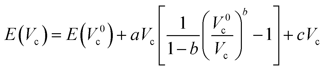
These modifications result in an increased energy E due to the Pauli repulsion and one can calculate the pressure on the system at different scaling factors by fitting the energies and cavity volumes to a Murnaghan equation of state, which analytically expresses this relationship in eqn (14) assuming a linear relationship between the bulk modulus and the pressure.101 The pressure is finally obtained as the derivative of this curve with respect to the cavity volume Vc, according to the thermodynamic relationship in eqn (15).
 | (14) |
 | (15) |
Apart from the electronic modifications considered thus far, an additional contribution to the energy is required to account for the creation of a molecular cavity in a pressurized medium.102–104 When calculating this contribution to H through the scaled particle theory of hard sphere fluids, this correction takes the form given in eqn (16) at a temperature of 0 K.
| H = E + pVc | (16) |
3. Computational details
XP-PCM calculations were performed on the main group elements between hydrogen and krypton at the DFT level of theory with the PBE0 hybrid functional105 using a Gaussian 16-interfaced106 in-house Julia code. The solvation was performed using the IEF-PCM107 formalism with cyclohexane as the solvent with a ζ solvent parameter set to 6 and a relative dielectric constant set to 1.0025 to minimize the electrostatic effects of solvation. The Rahm set of radii for neutral and monocharged atoms were used with a reference scaling factor f0 of 1.3.108 For H to Ar and Ga to Kr, the aug-cc-pVTZ109–114 basis set was used, while for K and Ca, the comparable 6-311++G(3df)115 basis set was employed since the aug-cc-pVTZ basis is not available for these elements. A concise study on the reliability of these settings is available in the ESI (SI.1).†To calculate the ionization potential and electron affinity, the parameters determined by the XP-PCM model for the neutral system are kept constant upon ionization in accordance with the expansion proposed in eqn (17). Because the cavity volume remains constant in this method as illustrated in Fig. 1a, it is denoted as ‘isochoric’. From a different point of view, the induced pressure on the system can be kept constant, resulting in an implicit constraint in eqn (17), where the XP-PCM parameters are imposed in such a way to keep the pressure constant. This method, denoted ‘isobaric’ and illustrated in Fig. 1b, involves separate XP-PCM calculations on the neutral and ionized systems starting from their respective radii and compares enthalpies at equal pressure. Results using this alternative method are supplied in the ESI (SI.3).† In the evaluation of the electronegativity, hardness and electron density, the explicit constraint is elected. It is important to remark that in both procedures the free electron in ionization processes is considered evacuated out of the pressurized system.
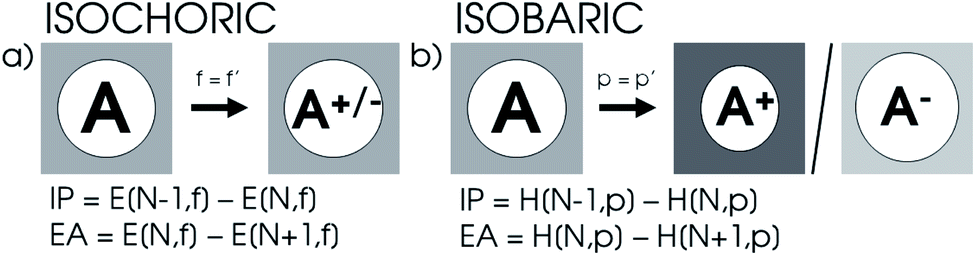 | ||
| Fig. 1 (a) Isochoric method for the calculation of ionization potential and electron affinity maintains XP-PCM parameters upon ionization. (b) Isobaric method for the calculation of ionization potential and electron affinity imposes an implicit constraint on the XP-PCM parameters by demanding the pressure in different calculations to be constant. | ||
For the calculation of the derivative of the energy with respect to pressure, a 4th order polynomial was fitted against the E(p) data and the derivative was calculated at the reference state. For this reference state, the starting situation at a scaling factor of 1.3 was chosen because it closely resembles standard solvation conditions (start of the XP-PCM model) and avoids errors due to the lack of tessellated surface in e.g. a gas phase calculation. This procedure showed excellent results with a Root Mean Square Error (RMSE) below 0.06 kcal mol−1 and this value improved little for higher order polynomials. The resulting derivatives matched well against numerical ones (between f = 1.3 and f = 1.25) and those obtained from logarithmic and exponential type fits against E(p) data, the latter two displaying a slightly higher RMSE (<0.3 and <0.7 kcal mol−1 for all elements, respectively). The derivatives of the enthalpy were obtained by fitting a 4th order polynomial to H(p) data (RMSE < 0.5 kcal mol−1) and taking the analytical derivative at the reference state. For the second derivative of the energy with respect to pressure, a Kumar equation of state was found to fit well to the date with an RMSE around 0.13 Å3, followed by analytical differentiation at the reference state. The second derivatives of enthalpy with respect to pressure at the reference state were obtained by fitting a third order polynomial to the V(p), V being the total volume  , data below 10 GPa, resulting in an average RMSE of 1.3 Å3. Mixed derivatives involving the electronegativity and chemical hardness were calculated using the finite difference approximation at the reference state (f = 1.3) and the subsequent point (f = 1.25). A similar finite difference approximation was followed for the pressure derivative of the isotropic polarizability, while the derivatives of the softness and cube of the softness were calculated starting from the numerical derivative of the hardness. Before evaluating the atomic electron densities, a sphericalization step was performed on the nonspherical atomic electron densities resulting from KS-DFT calculations on most atoms. This step comprised of a numerical averaging over polar angles θ and ϕ on a 20 by 10 grid by a python code interfaced with the Multiwfn program (version 3.8).116 RDFs were calculated, and the accuracy of the in-house code was validated by ensuring that ρ() integrated to N. Quantum Similarity Indices were finally computed numerically starting from the sphericalized densities as well as the Kullback–Leibler Information Deficiencies that were evaluated numerically after normalization of the electron density to 1 (shape function).
4. Results and discussion
4.1 Global response functions: response of the energy to pressure
Considering the change in energy when passing from one ground state to another (cf.eqn (1)), we now write: | (17) |
) still bears the meaning of the external potential as in the basic formalism of CDFT (eqn (1)), i.e. the potential due to the nuclei and all coefficients in the ΔE expression still bear the meaning of response functions. In the present work concentrating on atoms, or in the case of molecules, the pressure dependence of the electronic properties E, μ, η, … can safely be evaluated at constant v() if no relaxation of geometry is allowed.
Clearly, from a quantum mechanical point of view, the volume for atoms and molecules, while characteristic for the system, is not immediately defined and identifiable in real space. Despite this ambiguity in the interpretation of V, chemical intuition combined with some pragmatism suggests that chemical systems may be associated to a finite space around their position ![[R with combining right harpoon above (vector)]](https://www.rsc.org/images/entities/b_char_0052_20d1.gif) . An array of different numerical values have been proposed to quantify this feature, validated only by merit.108 While numerous arguments already exist, such as wavefunction criteria,108,117,118 trends in bond distances119 and non-contact radii in crystals120 and Pauli repulsion isosurfaces,121 we now introduce one rooted in the conceptual DFT framework, as implemented via the XP-PCM method. From the thermodynamic relationship
. An array of different numerical values have been proposed to quantify this feature, validated only by merit.108 While numerous arguments already exist, such as wavefunction criteria,108,117,118 trends in bond distances119 and non-contact radii in crystals120 and Pauli repulsion isosurfaces,121 we now introduce one rooted in the conceptual DFT framework, as implemented via the XP-PCM method. From the thermodynamic relationship  at 0 K, one expects the derivative of the enthalpy with respect to the pressure obtained from the XP-PCM model to yield the volume of the system. This can be separated into an electronic component
  , Velec, and a cavity component
  , according to eqn (16). Here, the first order derivative of the energy with respect to pressure
  is a leading new response function, which from a dimensional argument has the status of a volume analogous to e.g. the cavity volume Vc, a model parameter used as an adequate definition of the boundary in the XP-PCM model. Due to the Pauli repulsion, this response will evidently be positive for all systems and as a fundamental factor in the determination of the energy when perturbed by an external, isotropic pressure, this quantity is an intrinsic property of any electronic system, thus conveying relevant information about its structure and properties. It is rewarding to underline the analogy between the interpretation of
  as a volume and the identification of the corresponding derivative
  in a mechanochemical context,
 ![[F with combining right harpoon above (vector)]](https://www.rsc.org/images/entities/b_char_0046_20d1.gif) being the external mechanical force, as the (change in) equilibrium bond distance for diatomics.75
being the external mechanical force, as the (change in) equilibrium bond distance for diatomics.75
In Fig. 2, the volume  , V, and the electronic volume
  , Velec, at the reference state (f = 1.3) are provided for the atoms of all main group elements from hydrogen to krypton.
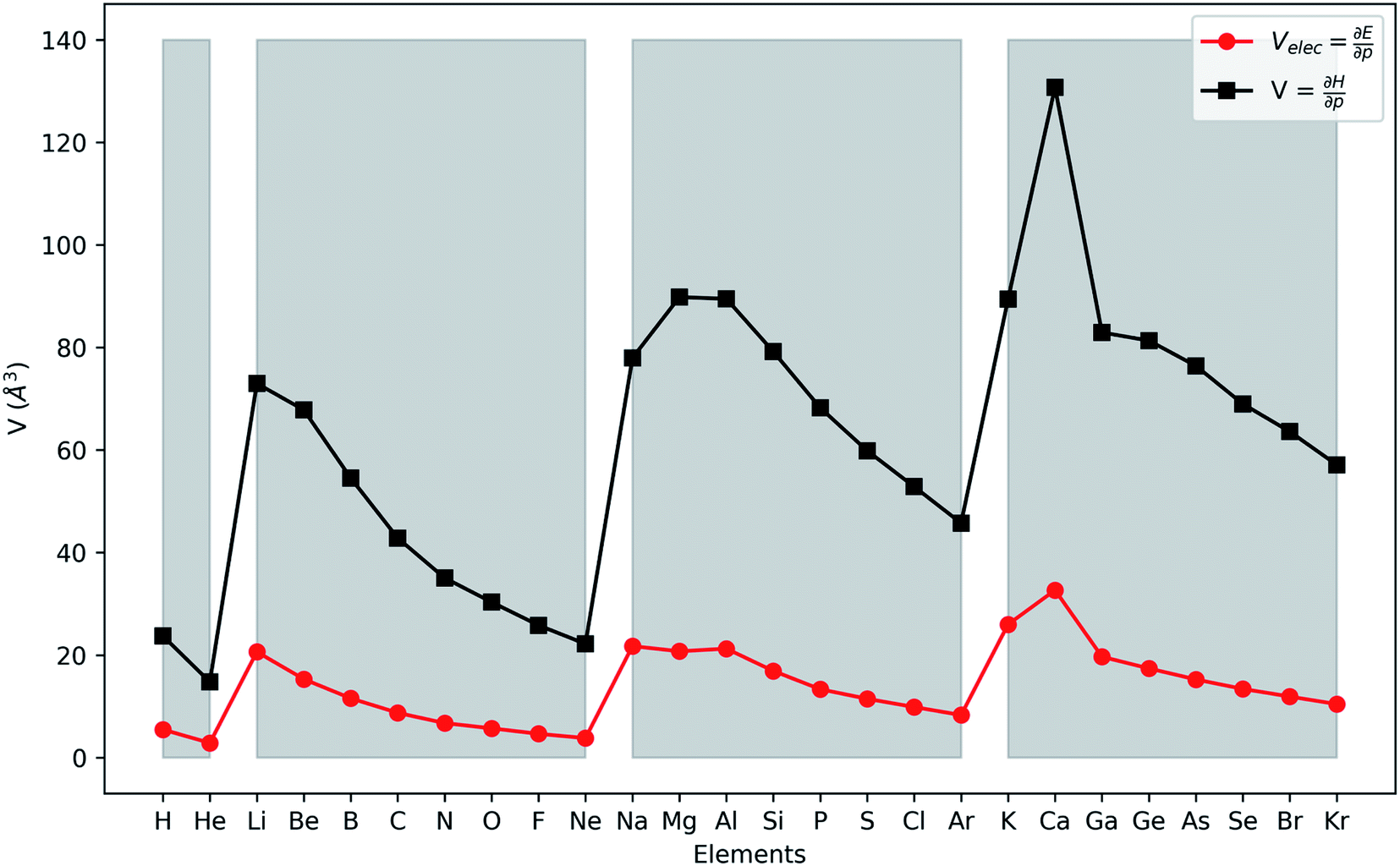 | ||
| Fig. 2 First derivative of the energy and enthalpy with respect to pressure for all main group elements from hydrogen to krypton. Grey zones group elements within one period of the periodic table. | ||
When compared against each other, the electronic volume is five to seven times smaller than its enthalpic counterpart, but generally follows the same trends. For both  and
and  , a decreasing trend can be found throughout a period, in agreement with the known contraction of atomic radii from the increasing effective nuclear charge. Additionally, both volumes identify helium as the smallest atom and calcium as the largest atom in this series. When moving to heavier periods, a systematic increase in atomic volume is found for both quantities, as expected for elements of the same group with more core electrons, but this effect is most outspoken for the atomic volume obtained through the enthalpy. When compared against experimental volumes of materials,122 no correlation could be retrieved, a first demonstration of the difference between atoms and materials. Combined, all these findings motivate the interpretation of the derivative of the electronic energy with pressure as a measure of the electronic atomic volume, quantifying the excluded space by the electrons from a pressurized medium and thus the extension of the atom.
To further establish the electronic atomic volume as a measure of the system size, a comparison to literature data can be made by defining a ‘pressure-sensitive radius’ as in eqn (18), where the pressure sensitivity refers to the origin of relec from a response to pressure. Here, an atom is modelled as a spherical entity of which the volume is set to the electronic volume obtained as the first-order derivative of the energy with respect to pressure. Note that this approach assumes sphericality which, while not retrieved for most atoms in the single reference wave function methods including Kohn–Sham DFT, is retrieved for the ground state by multireference methods.
 | (18) |
The radii relec are provided in Fig. 3a and the same periodic trend as for the volume is retrieved. The relec radii show fair correlations with most proposed sets of atomic radii, as seen in Fig. 3b–e and Table 1, but the best correlation is found with the Rahm set (Fig. 3b) for which a Pearson R2 coefficient of 0.907 was obtained.108 Another frequently used set of van der Waals radii, devised by Bondi, correlates worse with the relec values, but slightly better than with the Rahm set. This inferior correlation with the Bondi set is expected since, contrary to the Rahm set, Bondi radii are not derived from isolated atoms.120 Next the Ghosh set also retrieves a good, though nonlinear, correlation with our values, again anticipated because Ghosh radii are also associated with isolated atoms.118 Finally, the empirically motivated covalent set by Cordero retrieves, somewhat surprisingly, decent correlations with our pressure sensitive radii, comparable to those in between different sets.119 Overall, all these results establish the pressure sensitive radius as an adequate measure for the spatial extension of an atom.
 | ||
| Fig. 3 (a) Pressure-sensitive radius (relec) for all main group elements between hydrogen and krypton. Additionally, the correlation plots are supplied between the pressure sensitive radii and (b) the Rahm radii (triangles), (c) Bondi (squares), (d) Ghosh (pentagons) and (e) covalent radii (hexagons). Grey zones group elements within one period of the periodic table. | ||
| Pearson R2 | Rahm | Bondi | Ghosh | Covalent | r elec |
|---|---|---|---|---|---|
| Rahm | 1.000 | ||||
| Bondi | 0.542 | 1.000 | |||
| Ghosh | 0.548 | 0.723 | 1.000 | ||
| Covalent | 0.771 | 0.810 | 0.844 | 1.000 | |
| r elec | 0.907 | 0.586 | 0.753 | 0.828 | 1.000 |
Next to the first order response, second order derivatives with respect to pressure can be computed for both the energy and the enthalpy. While the second derivatives of the enthalpy could be computed using a polynomial fitting, values for the second derivative of the energy with respect to pressure showed a significant dependence on the order in this way. For this reason, an equation of state fitting approach inspired by the XP-PCM method of Cammi et al.99 was followed. This method starts from the first derivatives of the energy to pressure as obtained using the fitted 4th order polynomials and uses these as volumes in a high-pressure equation of state of the form developed by Kumar et al.:123
 | (19) |
Using a least square procedure to determine the parameters A, B0 and V0, the second derivative of the energy with respect to pressure could be obtained after differentiation of eqn (19) with respect to pressure, leading to eqn (20):
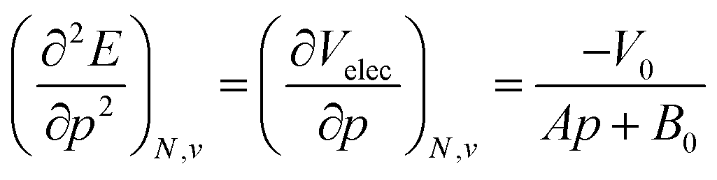 | (20) |
In Fig. 4, the second order response of the energy and enthalpy to pressure are provided for the main group elements hydrogen to krypton. Both display negative values, indicating that their respective atomic volumes and associated radii, both dependent on the pressure, decrease with increasing external pressure, as expected from chemical intuition. Periodicity again comes forth naturally with an increasing (decreasing absolute value) trend throughout a period, although exceptions can occur at the beginning of a period, some of them similar to exceptions in the generally decreasing first derivative. When compared against the pressure response of atomic volumes derived from the non-bonded radii under pressure by Rahm et al.,124 an expected, excellent agreement is found. Finally, making the same comparison to the volumes of elemental materials by Young et al.122 again no clear discernible trend could be obtained. Finally, the second derivative of the enthalpy is on average 5 times larger than that of the energy, similar to the relative magnitudes of the corresponding first order derivatives.
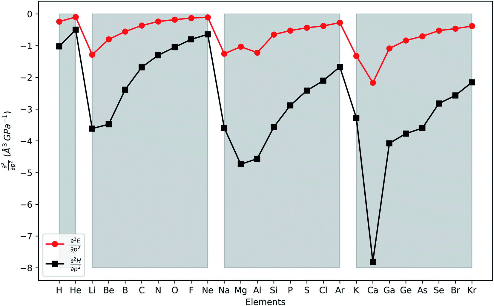 | ||
| Fig. 4 Second-order response of the enthalpy (black) and energy (red) with respect to pressure for all main group elements from hydrogen to krypton. Grey zones group elements within one period of the periodic table. | ||
This similar ratio has a direct consequence when considering the compressibility of these systems. In classical thermodynamics, the ratio of the opposite of the derivative of the volume with respect to pressure and the volume itself is defined as the compressibility κ, the inverse of the bulk modulus.125 The volume in the denominator is here introduced to modulate the second-order derivative to account for the differences in starting volume and the minus sign ensures an overall positive quantity. Transferring this concept to atomic systems, a separate enthalpic (κat–H) and electronic (κat–E) atomic compressibility can be defined by inserting the total atomic volume and electronic atomic volume, respectively.
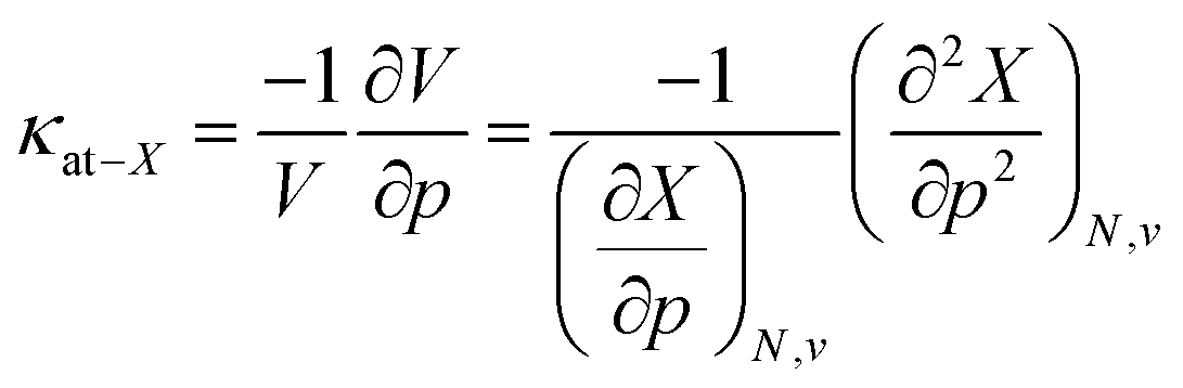 | (21) |
Atomic compressibilities for all main group elements from hydrogen to krypton are provided in the ESI (SI.2)† together with a comparison to reference data. Due to the aforementioned ratios between the enthalpy and energy derivatives for the elements considered, both compressibilities have similar magnitudes and display a decreasing trend throughout each period. A comparison to reference data shows a much higher variability (2–3 orders of magnitude) for experimental data than for the atomic compressibilities computed here (1 order of magnitude), suggesting that the compression of the atomic electron cloud cannot explain the total variability of material compressibilities. This aforementioned fundamental difference between atoms and materials can be ascribed to several factors. When considering isothermal compressibilities of solids,126 the presence of interstitial space, the different state of an atom in a solid compared to an isotropic fluid phase and the differences in crystal structure, among others, result in a poor correlation with our data. On the other hand, the effect of the crystal structure can be eliminated by a comparison with liquid metals at their respective melting point,127,128 but this introduces temperature differences as a new source of error. Accordingly, these data do not result in a good correlation with our atomic compressibilities.
4.2 Global response functions: ionization energy
In addition to the investigation of unmixed response functions, a number of mixed derivatives appear in the expansion in eqn (17) and the attention is now devoted to these properties in order to study the evolution of the traditional conceptual DFT response functions such as the electronegativity and chemical hardness under pressure. Prior to the evaluation of the response to external pressure of these conceptual DFT-based descriptors, their components, i.e. the ionization potential and the electron affinity, are evaluated. In Fig. 5a, the isochoric ionization potential is illustrated for the elements hydrogen to calcium and gallium to krypton. As expected from documented results on confinement, the ionization potential decreases with increasing pressure for all atoms and the curves display concave upward curvature, illustrating that the process of losing an electron becomes more favorable at high pressure.129,130 However, the rate of decrease is much lower compared to similar compressions for confinement models by a factor of 1.5 to 10. Additionally, the ordering of the atoms according to the ionization potential is retained over the considered pressure range with noble gases and halogens having the highest ionization potential and alkali metals having the lowest one. This unaltered pattern in periodicity indicates that the chemistry of ionization potentials at pressures up to 50 GPa remains unchanged. Finally, the influence of pressure on the ionization potential steadily decreases along a period with earlier elements being prone to the largest changes.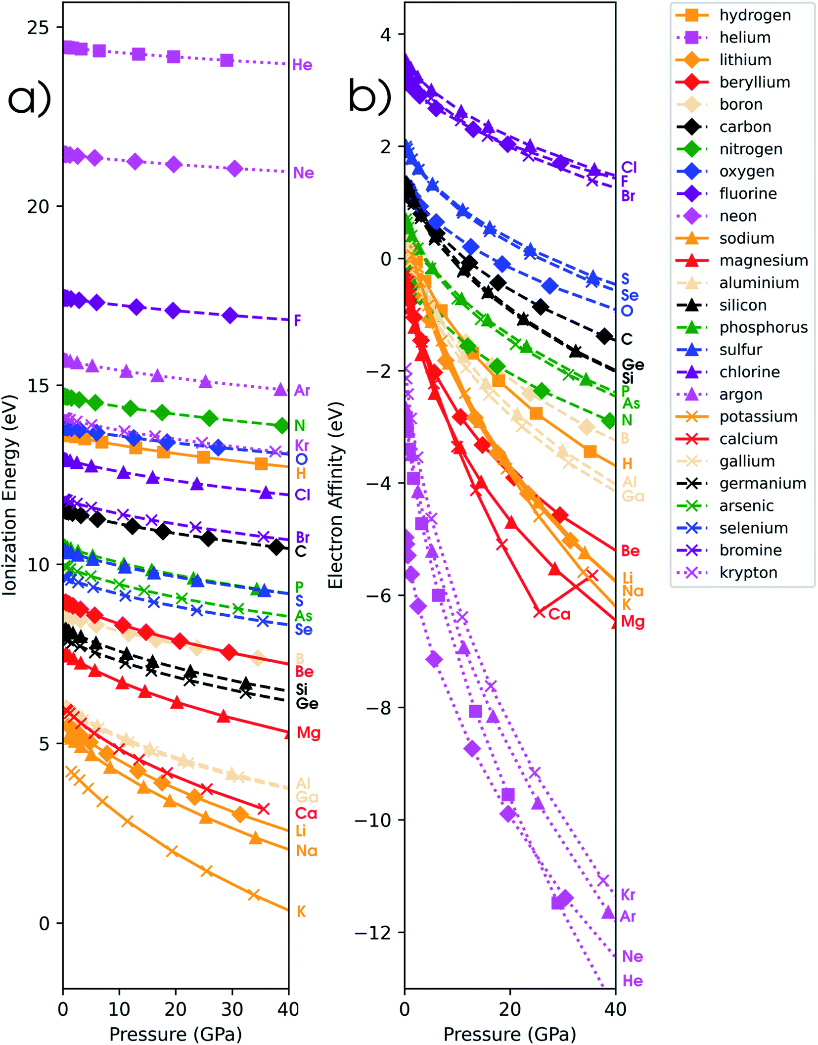 | ||
| Fig. 5 (a) Ionization potential as a function of pressure for all main group elements from hydrogen to krypton computed with the isochoric method. (b) Electron affinity as a function of pressure for all main group elements from hydrogen to krypton computed with the isochoric method. In both figures, the color of the curve denotes the group (Ia orange, IIa red, IIIa yellow, IVa black, Va green, VIa blue, VIIa purple, VIIIa magenta), the marker denotes the period (1 square, 2 diamond, 3 triangle, 4 cross) and the line style denotes the block (solid s-block, dashed p-block, dotted noble gases). | ||
While at ambient conditions all atoms are stable compared to their monocations and isolated electrons, it is not unthinkable that at some pressure the monocation will be the most stable state. This autoionization, leading to electrides, is known to exist under the influence of pressure; upon detachment, the electron occupies nonnuclear attractive regions or interstitial spaces in a crystal.42,131 The pressure at which this phenomenon could potentially occur was estimated through confinement studies for a series of second-row atoms and was found to vary between 17 GPa (Li) and 4131 GPa (Ne).129 In another study by Connerade et al., this autoionization process was investigated for 3rd and 4th period elements and was described as a consequence of the electron in the neutral state being bonded to the system cavity rather than the atom.132 In this work, the ionization pressure for electride formation is estimated via the XP-PCM method as the point where the energies of the neutral species and monocation become equal, resulting in a negative ionization potential for pressures higher than this critical value. Importantly, in this spontaneous ionization process, the electron is completely evacuated out of the pressurized system. This hypothetical situation is explored for a series of elements with low ionization potentials at ambient conditions and the autoionization pressures estimated using the isochoric method are provided in Table 2.
| Element | XP-PCM autoionization pressure | Confinement autoionization pressure129 | Experimental electride pressure |
|---|---|---|---|
| Lithium | 85 | 17 | 80 (ref. 133) |
| Beryllium | 327 | 119 | — |
| Boron | 481 | 200 | — |
| Carbon | 1016 | 527 | — |
| Sodium | 61 | — | 160 (ref. 134–137) |
| Magnesium | 189 | — | 800 (ref. 138) |
| Aluminium | 145 | — | — |
| Potassium | 45 | — | — |
| Gallium | 154 | — | — |
While the XP-PCM based model applied here is not intended to quantitatively determine electride pressures, often underestimating established values, it succeeds in retrieving two guiding principles of high pressure electrides. First, the lowest ionization pressures can be found for the alkali-metals and more generally, elements with low ionization potentials (see first rule in ref. 42). Secondly, atoms with valence electrons orbiting inner shells are more likely to form electrides, as illustrated by comparing magnesium and beryllium and aluminium and boron (see second rule in ref. 42). Interestingly, a very accurate prediction is obtained for the lithium atom, most likely due to error cancelation of the cavity reduction upon ionization (release of energy) by the generation of an interstitial electron (requires energy). Finally, when comparing the current method to confinement results,129 a similar trend throughout the first period is found, but with distinctly higher pressures.
4.3 Global response functions: electron affinity
In Fig. 5b, the electron affinity computed following the isochoric approach for the considered elements is given as a function of pressure. The process of gaining an electron becomes clearly more difficult with increasing pressure, as illustrated by the decreasing electron affinity for all elements. Eventually, the electron affinity becomes negative for most elements above 40 GPa; only the halogens retain a positive electron affinity. Note that some elements, such as Mg, Ca and noble gases, already exhibit a negative electron affinity without pressure. Negative values for the electron affinity are well known in computational chemistry and the problem of the interpretation of negative affinities is often solved by increasing the basis set and adding diffuse functions.139 This allows for the electron to be described loosely bound to the atom, eventually yielding an electron affinity of zero for a fully separated electron. This is, however, not the case within the XP-PCM formalism, where the Pauli potential prevents this situation. An illustration of the stability of the electron affinity with respect to increasing basis set size is provided in the ESI (SI.4).† In contrast to the ionization potentials, more crossings are found for the electron affinity. Notable examples include the oxygen atom which joins the other group VIa elements and nitrogen which does the same within group Va. An opposite trend is found for carbon and boron; however, both diverge away from their respective groups. Like the ionization potentials, the effects of pressure on the electron affinity decrease when moving through a period, apart from the noble gases which display a very steep decrease of the electron affinity due to the very unstable anion with increasing pressure. Finally, calcium displays an anomaly at approximately 30 GPa with an increasing electron affinity. This behavior can be explained by the configuration of the calcium anion changing from [Ar]4s24p1 to [Ar]4s23d1 in this pressure range, leading to a shallower increase of its energy and a transient rise in electron affinity.From the analysis of the ionization potential and electron affinity, these properties clearly depend on the pressure. This indicates that the chemistry of atoms at high pressure can differ substantially from the one observed at ambient conditions. To further put these findings in a conceptual DFT framework, the electronegativity χ, hardness η and electrophilicity ω were calculated. In the remainder of this work, the explicit constraint on the response functions in eqn (17) which directly keeps the set of XP-PCM parameters constant is preferred and thus the isochoric quantities are used.
4.4 Global response functions: electronegativity
In Fig. 6a, the conceptual DFT electronegativity of the considered elements are provided as a function of pressure. For all elements, the electronegativity decreases with increasing pressure with a concave upward curvature, resulting in a negative electronegativity for some elements at high pressure. This decreasing trend of the electronegativity with increasing pressure agrees well with the results obtained by Garza et al. for atoms confined in a Dirichlet type confining potential.140 Additionally, while all electronegativities decrease, the range in which they occur increases with pressure, that is, more electronegative elements display a less steep decrease than more electropositive elements. Both the general trend and shape of the curves in Fig. 6a agree with previous observations on the atomic electronegativity under pressure using a modified Allen scale.79 Further agreement with this scale can be found in the general lack of major crossings between atoms due to the absence of configurational changes in the considered pressure range. However, an important deviation from the results based on the Allen scale can be retrieved, namely the strong decrease of the electronegativities of the noble gases at high pressure. This decrease is mainly caused by the strong response of the electron affinity, as will be evident later. Finally, the case of calcium stands out: the sudden increase in electronegativity is caused by the corresponding artefact in the electron affinity component. | ||
| Fig. 6 (a) Electronegativity as a function of pressure for all main group elements from hydrogen to krypton computed with the isochoric method. (b) Chemical hardness as a function of pressure for all main group elements from hydrogen to krypton computed with the isochoric method. In both figures, the color of the curve denotes the group (Ia orange, IIa red, IIIa yellow, IVa black, Va green, VIa blue, VIIa purple, VIIIa magenta), the marker denotes the period (1 square, 2 diamond, 3 triangle, 4 cross) and the line style denotes the block (solid s-block, dashed p-block, dotted noble gases). | ||
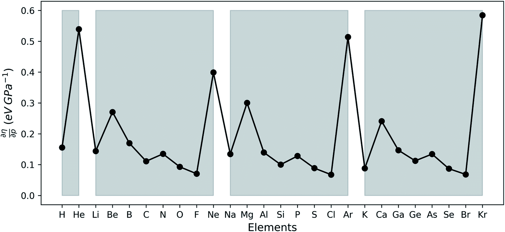
The periodic behavior and increasing range can be quantified by retaking the conceptual DFT expansion in eqn (17) from Section 3.1. Now mixed derivatives can be implemented to describe the evolution of reactivity descriptors and in Fig. 7, a first example of such a new response function is provided as 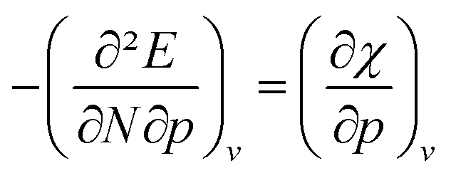 . The decreasing absolute value of the derivative in this figure along each period numerically demonstrates the accompanied decrease of the sensitivity of the electronegativity to pressure, resulting in a clear periodic behavior. This second-order response function is comparable to the electric field derivative of the electronegativity
 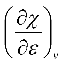 , generated in ref. 73 or the external force derivative in ref. 75.
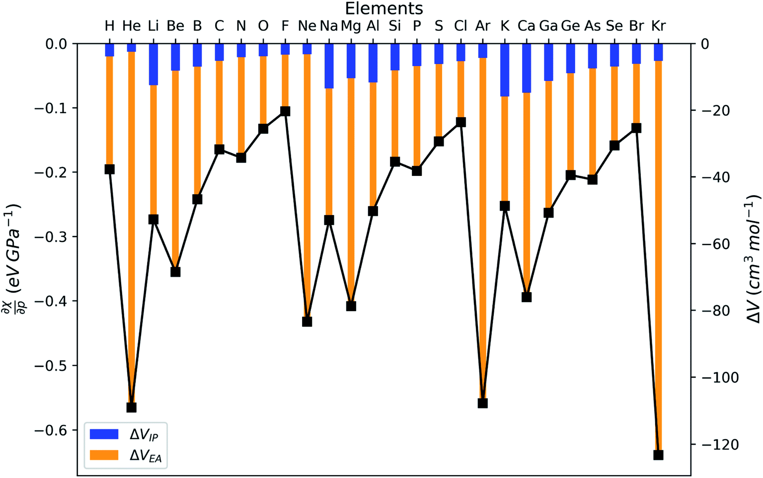 | ||
| Fig. 7 Derivative of the electronegativity as computed through the isochoric method with respect to the pressure at reference conditions (f = 1.3) calculated using the finite difference approximation (left axis) for all main group elements from hydrogen to krypton. The derivative is the sum of two volume components: one owing to the ionization potential (ΔVIP) and one owing to the electron affinity (ΔVEA) which are read from the right axis. | ||
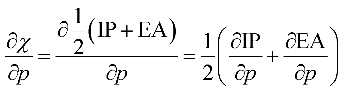
After implementing the working equation in eqn (2) into this derivative, one arrives at an expression for the derivative of the electronegativity as in eqn (22):
 | (22) |
After expanding the component energies of the ionization potential and electron affinity according to eqn (17) up to first order in the pressure, a few first-order energy derivatives come forth. As was shown in Section 3.1, these energy derivatives can be understood as electronic volumes (Velec), resulting in an expression:
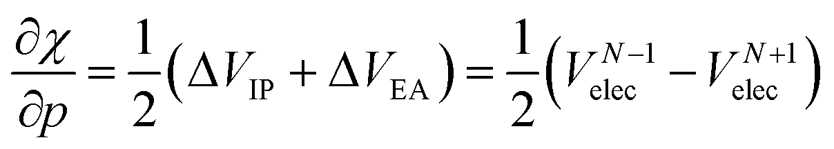 | (23) |
Because ΔVEA is larger than ΔVIP, a net positive reaction volume (ΔVion = ΔVIP(B) − ΔVEA(A)) can be associated to the hypothetical ionization reaction A + B → A− + B+. This result does not agree with the usual negative reaction volumes associated with ionization processes in solution ranging from −5 to −40 cm3 mol−1.12,13 This perceived discrepancy agrees with the general explanation for the cause of this negative volume, being the effects of electrostriction by the solvent.12 This effect known to influence reaction volumes in chemical processes, particularly when involving localized charges, small ions and apolar solvents, causes the entire solute–solvent ensemble to reduce its volume upon ionization due to enhanced interaction and thus induced approach between entities. This is not accounted for in the current implementation of the XP-PCM model based on isolated atoms and ions.
4.5 Global response functions: chemical hardness
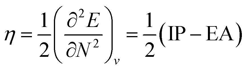
The (halved) difference of the ionization potential and electron affinity yields the chemical hardness (eqn (3)), recognized as in conceptual DFT. The chemical hardness increases with rising pressure (Fig. 6b), in line with prior literature data from confinement studies.140 Because the influence of pressure gradually diminishes, a convex upward curvature is found. An exception occurs for calcium which, due to the increase in electron affinity, displays a fall of the hardness around 30 GPa. Because of the varying steepness of the increase of the hardness for different elements, numerous crossings between elements can be observed, see for example the curves corresponding to hydrogen and magnesium. A notable example of such steep increases can be found in the noble gases, again due to the strong response of the electron affinity. This extreme position of the hardness (and electronegativity) of the noble gases is known to determine the chemistry of these elements.141 The extension of the conceptual DFT framework with respect to pressure now results in a third-order mixed derivative of the form
 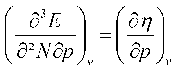 .
.
Analogous to the volume approach in Section 3.4, the derivative of the hardness can be separated into two components: 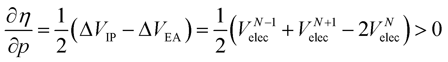 . Because the influence of ΔVEA was shown to be dominant over ΔVIP and ΔVEA being negative owing to the larger volume of an anion compared to a neutral system, the response of η with respect to p is positive for all elements. Fig. 9 indeed displays particularly high values for the noble gases and elements of group IIa, complementary to ΔVEA, while a generally decreasing trend is found within a period. Finally, no distinguishable trends in between different periods could be retrieved, the overall pattern displaying periodicity in the same way as
  .
.
Considering these data on the conceptual DFT descriptors on atoms of the elements under pressure, the question of how to transfer these concepts to molecules and the solid state naturally comes forth. Obviously, any scale of electronegativity and chemical hardness will have its limitations in predictive power, analogous to the situation at ambient conditions. At high pressure, the external potential, chemical environment and volume-work term are all involved in determining reactivity, complicating conclusions based on only electron transfer. Despite these effects, our data are expected to be applicable in studying general trends, bond polarities and as components in multivariate analyses. In the following section, we propose two examples of where our data succeed in explaining chemical behavior at high pressure.
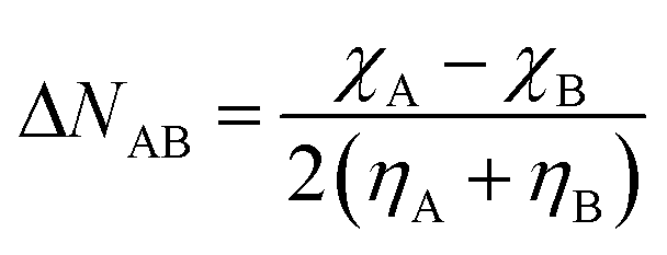
Because of the increased range in which the electronegativities occur at high pressure, an increased transfer of electrons and subsequent energy stabilization is intuitively expected in certain interatomic bonds. Within the conceptual DFT formalism, this transfer can be modelled by expanding the energy as a function of the number of electrons up to second order and finding the value for N−N0 (ΔN) at which the derivative of the total energy is zero. For a bond between atoms A and B, this results in a value for the electron transfer given by eqn (24), corresponding to Huheey's electronegativity equalization-based equation.142
 | (24) |
Since the electronegativity of the noble gases experiences a dramatic change with pressure, their bonds to electron-accepting bonding partners are expected to become more polarized in the direction of the electron acceptor. Such a pair has been identified in literature: the krypton–oxygen bond which is expected to yield stable compounds at high pressure.143 In Fig. 8a, the evolution of the electron transfer from krypton to oxygen is plotted as a function of pressure. Indeed, as pressure increases, an increased transfer of electrons and associated energy stabilization is expected to occur. A similar conclusion was obtained for this bond by Rahm et al. using the Allen electronegativity scale.79 A different example is illustrated by water and the predicted increase of its dipole moment under pressure by a range of computational models.43,144,145 This increase is also retrieved by our model as can be seen in Fig. 8b where the electron transfer in the hydrogen–oxygen bond is given as a function of pressure. For completeness, it is mentioned that our model for the dipole moment of water does not include the influence of pressure on the hydrogen–oxygen bond length and H–O–H bond angle.
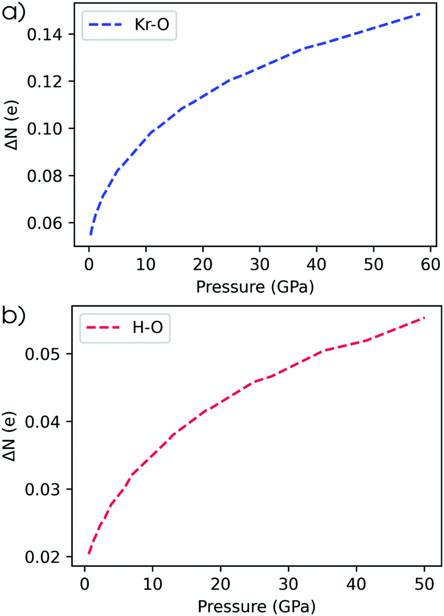 | ||
| Fig. 8 (a) Conceptual DFT electron transfer from krypton to oxygen. (b) Conceptual DFT electron transfer from hydrogen to oxygen. | ||
 | ||
| Fig. 9 Derivative of the chemical hardness as computed through the isochoric method with respect to the pressure at reference conditions (f = 1.3) calculated using the finite difference approximation for all main group elements from hydrogen to krypton. Grey zones group elements within one period of the periodic table. | ||
4.6 Global response functions: softness and polarizability
The softness is related to the chemical hardness as its inverse at 0 K. As the response of the hardness with pressure is positive, one can evidently expect softness to decrease with pressure for all elements. This behavior is apparent in its first-order derivative with respect to pressure as illustrated in Fig. 10a, where the derivative is calculated according to eqn (25) and the numerical derivatives of the hardness were used.
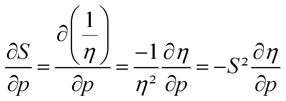 | (25) |
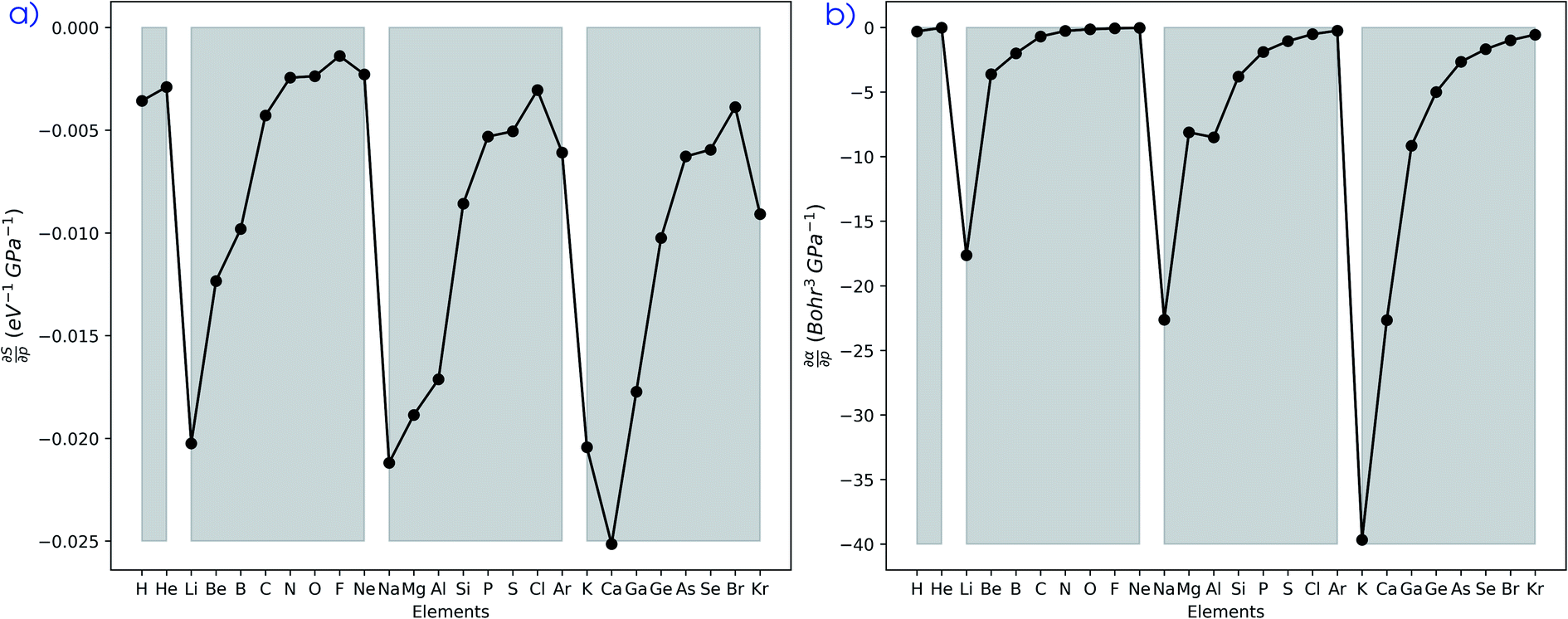 | ||
| Fig. 10 (a) Derivative of the softness as computed through the isochoric method with respect to the pressure at reference conditions (f = 1.3) calculated using eqn (25) for all main group elements from hydrogen to krypton. (b) Derivative of the isotropic polarizability with respect to the pressure at reference conditions (f = 1.3) calculated using the finite difference approximation for all main group elements from hydrogen to krypton. Grey zones group elements within one period of the periodic table. | ||
Evidently, all softness derivatives are negative, indicating a decreasing trend with pressure and the halogens still come forth as having the least sensitive softness with respect to pressure. Additionally, the hard character of the noble gases at standard conditions results in a softness derivative that is comparable to the heavier elements (group Va to VIIa) within a period. Finally, the most sensitive softness is obtained for the group Ia metals, except for calcium whose relatively soft nature leads to a very negative derivative.
The well-known relationship at ambient conditions between the cube of the softness S3 and the isotropic polarizability α incited us to investigate, for a given element, the same relationship as a function of pressure. First, the derivative of the polarizability with respect to pressure  is calculated in Fig. 10b which shows negative values as expected from the well-known decrease of the polarizability upon confinement.35,146 A periodic trend is observed with the most sensitive polarizabilities for the alkali metals with large negative values. Note the exceptionally small jump when passing from magnesium to aluminum, while other transitions from the s block to the p block only result in slight discontinuities. Coming back to the relationship between softness and polarizability, a previous study on atomic confinement found good correlations between S3 and α for a given atom when varying the confinement radius.146 To quantify the correlation between S3 and α, we used the Pearson correlation R2 and P-value of the slope or the Spearman rank correlation coefficient for the cases where linearity and homoscedasticity are not fulfilled. For all elements, a Spearman rank correlation coefficient of 1 is found, except for calcium due to the artefact in the hardness. Additionally, excellent Pearson R2 values can be retrieved ranging from 0.9626 to 0.9999. The best correlation is found for carbon (Fig. 11a), sodium, aluminum, arsenic and selenium, while the noble gases generally display worse correlations with deviations from a linear trend (SI.5).† The overall conclusion is that the relationship between S3 and α for a given atom of an element, persists when changing the external pressure. To consider this relationship between different elements at different pressures, both sides can be differentiated with respect to pressure, leading to an expected correlation between
  and
and  . This plot is shown in Fig. 11b and a good correlation is found with a Pearson R2 coefficient of 0.94, raising evidence for the general S3 ∼ α at different pressures. The reduced correlation compared to single elements can at least in part be ascribed to the varying number of valence electrons of different elements.89
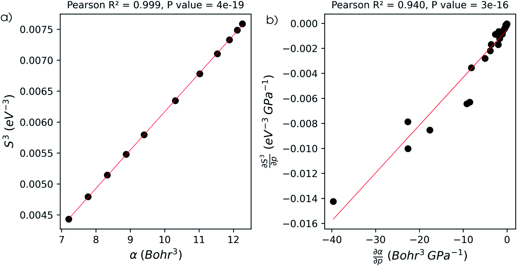 | ||
| Fig. 11 (a) Correlation between the cube of the softness as computed through the isochoric method and the isotropic polarizability for a carbon atom under pressure up to 50 GPa. (b) Correlation between the derivative of the isotropic polarizability and the cube of the softness as computed through the isochoric method with respect to pressure. Both data points and linear regression line are plotted. | ||
4.7 Global response functions: electrophilicity index
Through a combination of the response of the electronegativity and the chemical hardness, the electrophilicity index can be computed as a function of pressure (eqn (4)). Because the electronegativity of certain elements (e.g. alkali-metals) reaches negative values in the considered pressure range, their electrophilicity will eventually increase again parabolically, posing a problem in its interpretation. When EA < −IP, the direction of the electron exchange with an infinite, zero chemical potential electron sea inverts and the concomitant energy stabilization increases again. The two parabola model by Gazquez et al.147 allows to postpone this problem for the electrodonating power (ω−) until EA < −3·IP, but does not eliminate it.In Fig. 12, the electrophilicity index is given for the elements for which the −IP < EA condition is fulfilled in the considered pressure range. These constitute the majority of the p block elements and all their electrophilicities decrease steeply with convex curvature, confirming that all these atoms become less electrophilic with respect to the vacuum at increased pressure.
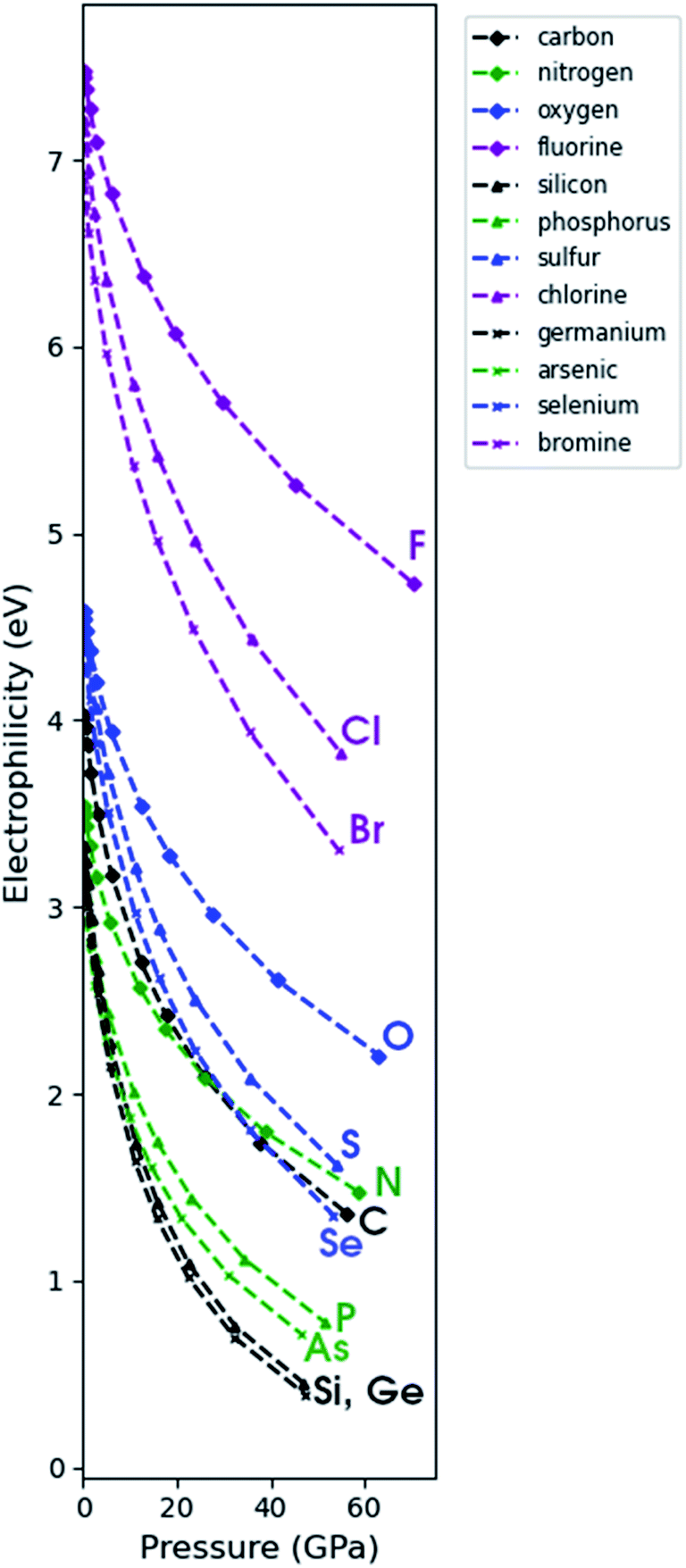 | ||
| Fig. 12 Electrophilicity index as computed through the isochoric method as a function of pressure for group IVa, Va, VIa and VIIa for the 2nd, 3rd and 4th period. | ||
For the sake of completeness and to finish this part on global descriptors, the relative deviations of the Kohn–Sham orbital energies due to pressure are provided in the ESI (SI.6).†
4.8 The electron density: the radial distribution function
Next to the global reactivity descriptors, the local response function of interest in this work is the electron density. Because increased pressure leads to an increase of the density near the nucleus for all atoms, the radial distribution function is employed to illustrate the shift of electron density as a function of the distance to the nucleus r. The evolution of the RDF for a hydrogen atom is shown in Fig. 13a and the difference compared to the RDF at reference conditions (f = 1.3) is given in Fig. 13b. A clear shift of electron density is found from the external regions of the atom toward the internal regions with a maximum increase around the maximum of the RDF. The former effect was already described by Cammi et al. for a butadiene molecule and matches chemical intuition.44 The maximum decrease is generally aligned with the boundary of the pressurized cavity, which is illustrated by dotted vertical lines in Fig. 13b. Similar trends can be observed for the main group elements from helium to krypton, for which the RDF and difference in RDF are provided in the ESI (SI.7 & SI.8, respectively†). In alkali and alkaline-earth metals, however, exceptions were found where the maximum decrease is located outside of the cavity. Additionally, in the internal regions of heavier atoms, slight oscillations occur in the difference in RDF that are most distinct for s-block elements but present in all elements. The maxima of these oscillations can be found at the subshell maxima of the RDF, while the minima are located at inter(sub)shell minima, resulting in a constant or even decreased probability to find electrons in this region.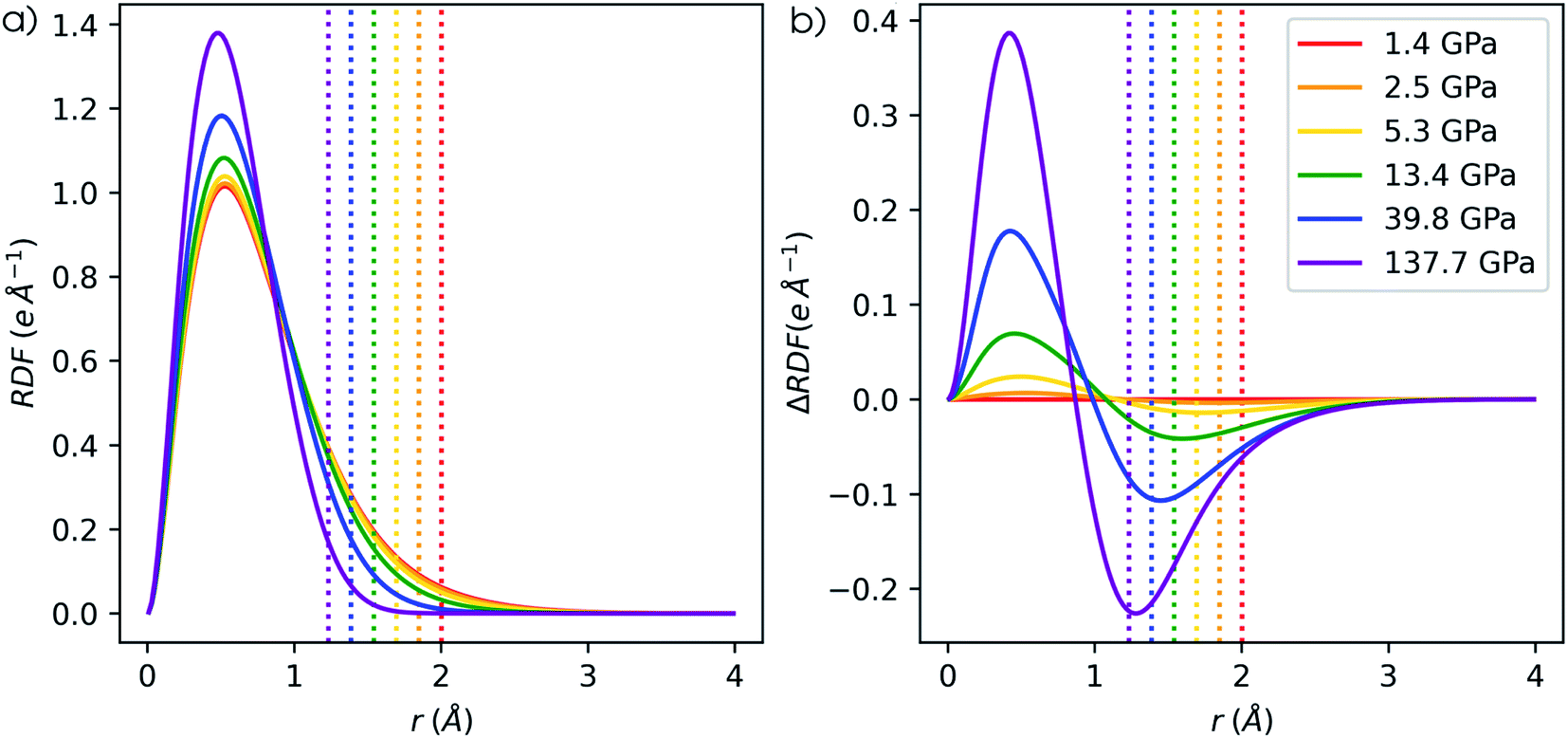 | ||
| Fig. 13 (a) Radial distribution of a hydrogen atom under pressure. (b) Difference in radial distribution of hydrogen atom under pressure compared to reference conditions (f = 1.3). Vertical dotted lines indicate the cavity radius. | ||
Additionally, the redistribution of electron density from the outer to the inner regions when going from 1 to 50 GPa is most evident for the elements early on in a period. To quantify the shift in radial distribution from the peripheral to the internal regions, the total increase of electron density in the inner region (ΔNRDF) is quantified using eqn (26). Here, the inner region ranges from 0 to r, where r is taken as the radius which maximizes the integrand, being the RDF at 50 GPa compared to the reference state (f = 1.3).
 | (26) |
The results for the main group elements from hydrogen to krypton are provided in Fig. 14 and retrieve clear periodicity with a stronger shift in electron density from the outer to the inner regions for the earlier elements within a period. In between different periods, a generally larger shift is found for lower periods, which can be partially attributed to their larger number of electrons.
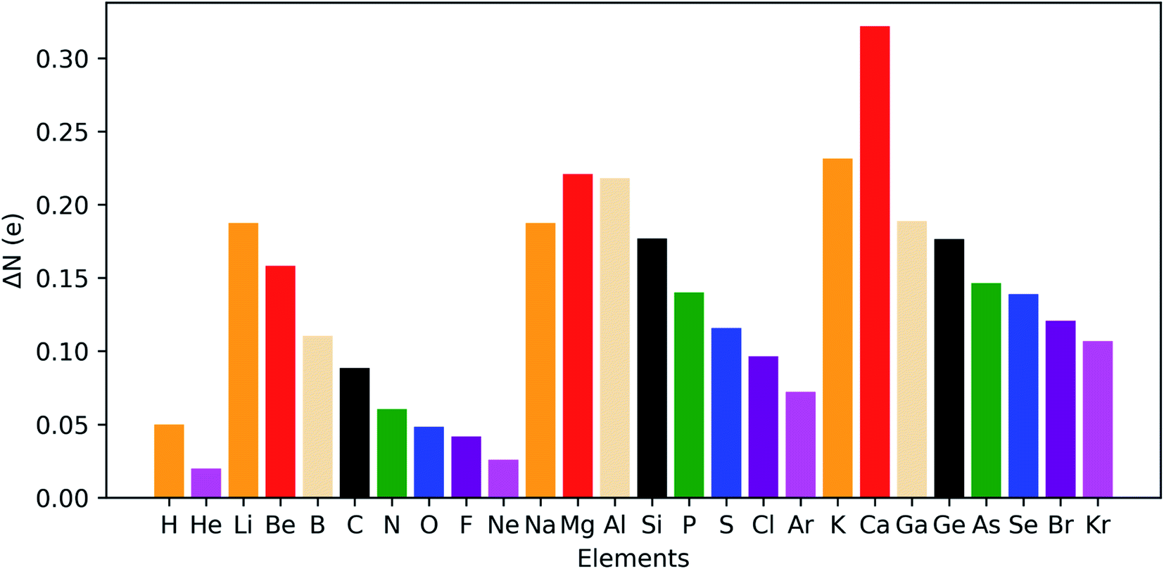 | ||
| Fig. 14 Maximal shift in electron density from outer to inner region of atoms at 50 GPa compared to reference conditions (f = 1.3) for all main group elements from hydrogen to krypton. | ||
4.9 The electron density: Carbó similarity and Kullback–Leibler information deficiency
The second method to investigate the evolution of the electron density is based on the Carbó quantum similarity index, which compares the density at some pressure to the one at reference conditions (f = 1.3). In Fig. 15a, the evolution of the QSI is given for a hydrogen atom as a function of pressure. While this index is rather unsensitive to small changes, a monotonic decreasing trend can be obtained, indicating the decreasing similarity to the reference. When expanding this approach to the main group elements between hydrogen and krypton in Fig. 15b, a strongly increasing similarity for heavier elements is found when comparing the situation at 50 GPa and the reference situation. This is due to the relatively small changes of the density for atoms with many electrons. Although the overall trend between the heavier elements is faint, clear periodicity is retrieved when passing to a logarithmic scale in Fig. 15c. Calcium stands out and displays a lower QSI than its predecessor potassium, indicating that it is more sensitive to pressure against the general trend.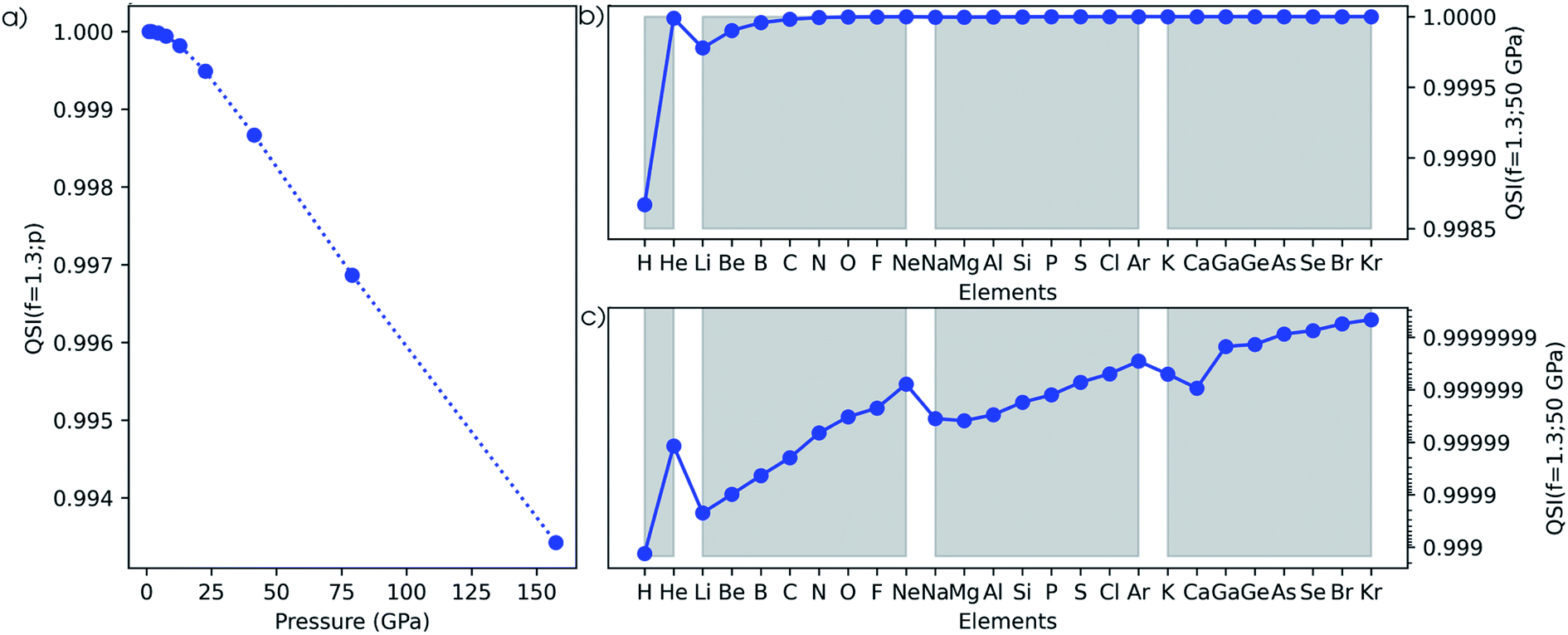 | ||
| Fig. 15 (a) Evolution of the Carbó similarity index (QSI) for the hydrogen atom as a function of pressure compared to the reference condition (f = 1.3). (b) Carbó similarity index at 50 GPa compared to the reference conditions (f = 1.3) for all main group elements from hydrogen to krypton. (c) Logarithmic scale of Carbó similarity index at 50 GPa compared to the reference conditions (f = 1.3) for all main group elements from hydrogen to krypton. Grey zones group elements within one period of the periodic table. | ||
The third measure to compare the electron densities is the Kullback–Leibler information deficiency (ΔSKL, eqn (8)) which quantifies the dissimilarity or missing information between shape functions. In Fig. 16a, the information deficiency is given for the hydrogen atom as a function of pressure, resulting in a monotonic increase in the dissimilarity with pressure, in agreement with the Carbó QSI. In Fig. 16b, the information deficiency is provided for the main group elements between hydrogen and krypton. Here, the decrease of ΔSKL within a period indicates a lower sensitivity of the electron density to pressure for early-period elements, in agreement with the results of the RDF and the Carbó QSI. Compared to the Carbó QSI, a clearer picture emerges due to the higher sensitivity of this index to small changes. In between periods, trends are less evident, but generally a decreased effect of pressure is observed. Again, calcium does not follow the general trend, analogous to the Carbó QSI. Finally, it is worth mentioning that contrary to previous studies that identified periodicity in the electron density of the atomic elements through the information deficiency, herein no prior bias is introduced due to discrete changes in the shape function used for comparison σ0().95 Overall, the different methodologies to study the effects of pressure on the electron density of atoms unanimously indicate a shift of electron density from the outer to the inner regions of an atom, with an increased sensitivity to pressure for early elements in a given period.
 | ||
| Fig. 16 (a) Evolution of the Kullback–Leibler Information Deficiency for the hydrogen atom as a function of pressure compared to the reference condition (f = 1.3). (b) Kullback–Leibler information deficiency at 50 GPa compared to reference conditions (f = 1.3) for all main group elements from hydrogen to krypton. Grey zones group elements within one period of the periodic table. | ||
5. Conclusion
In this work, the conceptual DFT framework has been extended to include pressure and the concomitant new response functions have been examined for the main group atoms from hydrogen to krypton. Using the XP-PCM method, the first-order response of the energy with respect to pressure was identified as the electronic atomic volume, an intrinsic property of an atom, and allowed to derive a new pressure-sensitive atomic radius which correlates well with existing data sets of atomic radii. The second-order response functions were linked to atomic compressibilities, the analogue of the compressibility for macroscopic systems. The ionization potential decreases with increasing pressure, but the overall sequence of standard pressure values is preserved. However, elements with lower ionization potentials experience a stronger decrease than elements with higher potentials, thus broadening the overall range. Similarly, the electron affinity decreases with rising pressure but more intersections between different elements are observed. Again, a broadening of the range occurs at increased pressure. A different method to calculate the ionization potentials and electron affinities denoted as the isobaric method found similar trends but generally estimated the ionization potentials and electron affinities to be lower than their isochoric counterparts at any pressure. Combining these two quantities, the electronegativity was found to decrease with increasing pressure for all elements. The first derivative of the electronegativity with respect to pressure indicates that elements early on in a period are more sensitive to pressure than those later on in the period, except for the noble gases. The interpretation of the first-order response of the energy with respect to pressure as an electronic volume allowed to interpret the trends in the derivative of the electronegativity. The chemical hardness increases with pressure for all elements and its pressure derivative confirms this picture with a periodic trend of decreasing sensitivity to pressure for heavier elements, in particular for alkaline earth metals and noble gases. The softness and isotropic polarizability decrease upon increasing pressure with lowering sensitivity throughout a period. The relationship between the isotropic polarizability and the cube of the softness is maintained with varying pressure. The electrophilicity decreases for higher pressure conditions but can reach zero before increasing again due to negative electronegativities. The interpretation of the electrophilicity is therefore ambiguous and this descriptor in its current definition is at risk for misinterpretation when describing the reactivity of a chemical system for which the −IP < EA condition is not fulfilled at extreme pressure conditions. For all global properties, periodicity is retrieved in a natural way. Despite the limitations innate to any set of reactivity descriptors, the evolution of the global reactivity descriptors in our atom based model proved capable of retrieving some general rules and striking findings in high pressure chemistry, including results on auto-ionization, the stability of Kr–O bonds and the increase of the dipole moment of H2O at high pressure.To compare electron densities, three different methods were used. The radial distribution function showed that the electron density of atoms is more concentrated near the maximum of the RDF as pressure increases, while the maximum depletion is generally located around the cavity boundary. The total shift in electron density from the outer to inner regions decreases throughout a period, displaying clear periodic behavior. The overlap-like Carbó quantum similarity index showed a monotonic decrease in similarity of the electron density for the hydrogen atom with pressure and retrieved some periodicity, although being dominated by the decreasing relative change due to the increasing number of electrons. The Kullback–Leibler information deficiency showed a monotonically increasing dissimilarity for the electron density of the hydrogen atom under pressure and a decreasing sensitivity to pressure for the electron density throughout a period. An overall unbiased periodic pattern shows up.
The overall findings in this extension of the conceptual DFT framework to include pressure in the case of atoms may offer guiding principles for the investigation of pressure effects on the reactivity of molecules and is actively being studied in our research group.
Data availability
Data available on request.Author contributions
J. E. performed all the calculations and J. E. and B. C. wrote the required scripts. All authors were involved in the conceptualization of the study and in the analysis of the results. The supervision was done by P. G., M. A. and F. D. P. The first draft was written by J. E. and all authors were involved in the further editing and reviewing process.Conflicts of interest
There are no conflicts to declare.Acknowledgements
J. E. acknowledges support by the FWO (Fund for Scientific Research-Flanders) under grant number 1148522N. M. A. thanks the Fund for Scientific Research-Flanders (FWO-12F4416N) for a postdoctoral fellowship and the Vrije Universiteit Brussel (VUB) for financial support. Computational resources and services were provided by the shared ICT Services Centre funded by the Vrije Universiteit Brussel, the Flemish Supercomputer Center (VSC) and FWO. The authors also want to acknowledge the Vrije Universiteit Brussel for the support through a Strategic Research Program (SRP). Finally, the authors thank the reviewers for their useful and insightful comments on our initial manuscript, which have undoubtedly increased the quality of this work.References
- E. H. Amagat, Memoires sur l'Élasticité & la Dilatabilité des Fluides jusqu'aux très Hautes Pressions, Gauthier-Villars, 1893 Search PubMed.
- T. Andrews, Rep. Br. Assoc. Adv. Sci., 1861, 31 Search PubMed.
- F. M. Raoult, Sur les Tensions de Vapeur des Dissolutions, Impremerie Gauthier-Villars et fils, 1890 Search PubMed.
- A. S. Travis, in Determinants in the Evolution of the European Chemical Industry, 1900-1939, chemists and chemistry, Springer, Dordrecht, 1998, pp. 3–21 Search PubMed.
- R. Winter and W. Dzwolak, Philos. Trans. R. Soc., A, 2005, 363, 537–563 CrossRef CAS PubMed.
- J. Zhang, X. Peng, A. Jonas and J. Jonas, Biochemistry, 1995, 34, 8631–8641 CrossRef CAS PubMed.
- L. Smeller, Biochim. Biophys. Acta, 2002, 1595, 11–29 CrossRef CAS.
- J. Roche, J. M. Louis, A. Bax and R. B. Best, Proteins, 2015, 83, 2117–2123 CrossRef CAS PubMed.
- P. Mentré and G. H. B. Hoa, Int. Rev. Cytol., 2001, 1–84 Search PubMed.
- T. Asano and W. J. Le Noble, Chem. Rev., 1978, 78, 407–489 CrossRef CAS.
- V. Schettino and R. Bini, Chem. Soc. Rev., 2007, 36, 869–880 RSC.
- R. Van Eldik, T. Asano and W. J. Le Noble, Chem. Rev., 1989, 89, 549–688 CrossRef CAS.
- B. Chen, R. Hoffmann and R. Cammi, Angew. Chem., Int. Ed., 2017, 56, 11126–11142 CrossRef CAS PubMed.
- W. J. Le Noble, in High Pressure Chemistry and Biochemistry, Springer, Dordrecht, 1987, pp. 295–310 Search PubMed.
- G. Jenner, in High Pressure Chemistry, Biochemistry and Materials Science, Springer, Dordrecht, 1993, pp. 367–392 Search PubMed.
- G. Jenner, New J. Chem., 1999, 23, 525–529 RSC.
- F. G. Klärner and F. Wurche, J. Prakt. Chem., 2000, 342, 609–636 CrossRef.
- P. F. McMillan, Chem. Soc. Rev., 2006, 35, 855–857 RSC.
- W. Grochala, R. Hoffmann, J. Feng and N. W. Ashcroft, Angew. Chem., Int. Ed., 2007, 46, 3620–3642 CrossRef CAS PubMed.
- R. J. Hemley, Annu. Rev. Phys. Chem., 2000, 51, 763–800 CrossRef CAS PubMed.
- G. Demazeau, Z. Naturforsch., B: J. Chem. Sci., 2006, 61, 799–807 CrossRef CAS.
- P. Postorino and L. Malavasi, MRS Bull., 2017, 42, 718–723 CrossRef CAS.
- J. Lin, X. Du and G. Yang, Chin. Phys. B, 2019, 28, 106106 CrossRef CAS.
- E. Wigner and H. B. Huntington, J. Chem. Phys., 1935, 3, 764–770 CrossRef CAS.
- R. J. Hemley, Z. G. Soos, M. Hanfland and H.-K. Mao, Nature, 1994, 369, 384–387 CrossRef CAS.
- J. McMinis, R. C. Clay, D. Lee and M. A. Morales, Phys. Rev. Lett., 2015, 114, 105305 CrossRef PubMed.
- D. M. Newitt, Biogr. Mem. Fellows R. Soc., 1962, 8, 26–40 CrossRef.
- S. Anzellini and S. Boccato, Crystals, 2020, 10, 459 CrossRef CAS.
- B. Li, C. Ji, W. Yang, J. Wang, K. Yang, R. Xu, W. Liu, Z. Cai, J. Chen and H. Mao, Proc. Natl. Acad. Sci. U. S. A., 2018, 115, 1713–1717 CrossRef CAS PubMed.
- J. Li, I. M. Chou, W. A. Bassett and X. Wang, Rev. Sci. Instrum., 2020, 91, 053104 CrossRef CAS PubMed.
- J. R. Asay and M. Shahinpoor, High-Pressure Shock Compression of Solids, Springer Science & Business Media, 2012 Search PubMed.
- R. A. Graham, Solids Under High-Pressure Shock Compression: Mechanics, Physics, and Chemistry, Springer Science & Business Media, 2012 Search PubMed.
- N. Aquino, Adv. Quantum Chem., 2009, 57, 123–171 CrossRef CAS.
- A. Michels, J. De Boer and A. Bijl, Physica, 1937, 4, 981–994 CrossRef CAS.
- P. Geerlings, D. J. Tozer and F. De Proft, in Chemical Reactivity in Confined Systems: Theory, Modelling and Application, John Wiley, New York, 2021, ch. 3 Search PubMed.
- I. R. McDonald, Mol. Phys., 1972, 23, 41–58 CrossRef CAS.
- H. C. Andersen, J. Chem. Phys., 1980, 72, 2384–2393 CrossRef CAS.
- W. G. Hoover, Phys. Rev. A, 1986, 34, 2499–2500 CrossRef PubMed.
- G. J. Martyna, D. J. Tobias and M. L. Klein, J. Chem. Phys., 1994, 101, 4177–4189 CrossRef CAS.
- G. Subramanian, N. Mathew and J. Leiding, J. Chem. Phys., 2015, 143, 134109 CrossRef PubMed.
- T. Stauch, R. Chakraborty and M. Head-Gordon, ChemPhysChem, 2019, 20, 2742–2747 CrossRef CAS PubMed.
- M. S. Miao and R. Hoffmann, Acc. Chem. Res., 2014, 47, 1311–1317 CrossRef CAS PubMed.
- M. Scheurer, A. Dreuw, E. Epifanovsky, M. Head-Gordon and T. Stauch, J. Chem. Theory Comput., 2021, 17, 583–597 CrossRef CAS PubMed.
- R. Cammi, V. Verdolino, B. Mennucci and J. Tomasi, Chem. Phys., 2008, 344, 135–141 CrossRef CAS.
- R. Cammi, J. Comput. Chem., 2015, 36, 2246–2259 CrossRef CAS PubMed.
- R. Cammi, C. Cappelli, B. Mennucci and J. Tomasi, J. Chem. Phys., 2012, 137, 154112 CrossRef CAS PubMed.
- M. Pagliai, G. Cardini and R. Cammi, J. Phys. Chem. A, 2014, 118, 5089–5111 CrossRef PubMed.
- R. Fukuda, M. Ehara and R. Cammi, J. Chem. Theory Comput., 2015, 11, 2063–2076 CrossRef CAS PubMed.
- R. Cammi and B. Chen, Annu. Rep. Comput. Chem., 2021, 17, 3–22 Search PubMed.
- W. Zhang, A. R. Oganov, A. F. Goncharov, Q. Zhu, S. E. Boulfelfel, A. O. Lyakov, E. Stavrou, M. Somayazulu, V. B. Frakapenka and Z. Konopkova, Science, 2013, 342, 1502–1505 CrossRef CAS PubMed.
- E. Zurek, R. Hoffmann, N. W. Ashcroft, A. R. Oganov and A. O. Lyakhov, Proc. Natl. Acad. Sci. U. S. A., 2009, 106, 17640–17643 CrossRef CAS PubMed.
- V. A. Mukhanov, O. O. Kurakevych and V. L. Solozhenko, J. Superhard Mater., 2010, 32, 167–176 CrossRef.
- Q. Li, Y. Ma, A. R. Oganov, H. Wang, H. Wang, Y. Xu, T. Cui, H. K. Mao and G. Zou, Phys. Rev. Lett., 2009, 102, 175506 CrossRef PubMed.
- W. L. Mao, Science, 2003, 302, 425–427 CrossRef CAS PubMed.
- H. Wang, J. S. Tse, K. Tanaka, T. Iitaka and Y. Ma, Proc. Natl. Acad. Sci. U. S. A., 2012, 109, 6463–6466 CrossRef CAS PubMed.
- A. P. Drozdov, P. P. Kong, V. S. Minkov, S. P. Besedin, M. A. Kuzovnikov, S. Mozaffari, L. Balicas, F. F. Balakirev, D. E. Graf, V. B. Prakapenka, E. Greenberg, D. A. Knyazev, M. Tkacz and M. I. Eremets, Nature, 2019, 569, 528–531 CrossRef CAS PubMed.
- H. Liu, I. I. Naumov, R. Hoffmann, N. W. Ashcroft and R. J. Hemley, Proc. Natl. Acad. Sci. U. S. A., 2017, 114, 6990–6995 CrossRef CAS PubMed.
- G. Gao, R. Hoffmann, N. W. Ashcroft, H. Liu, A. Bergara and Y. Ma, Phys. Rev. B: Condens. Matter Mater. Phys., 2013, 88, 184104 CrossRef.
- Y. Li, J. Hao, H. Liu, Y. Li and Y. Ma, J. Chem. Phys., 2014, 140, 174712 CrossRef PubMed.
- D. T. Hawkins, J. Chem. Inf. Model., 1978, 18, 190–199 CrossRef CAS.
- Z. Mazej, Molecules, 2020, 25, 3014 CrossRef CAS PubMed.
- L. Graham, O. Graudejus, N. K. Jha and N. Bartlett, Coord. Chem. Rev., 2000, 197, 321–334 CrossRef CAS.
- P. Hohenberg and W. Kohn, Phys. Rev., 1964, 136, 864–871 CrossRef.
- R. G. Parr, R. A. Donnelly, M. Levy and W. E. Palke, J. Chem. Phys., 1978, 68, 3801–3807 CrossRef CAS.
- R. G. Parr and W. Yang, Density Functional Theory of Atoms and Molecules, Oxford University Press, Oxford, 1989 Search PubMed.
- H. Chermette, J. Comput. Chem., 1999, 20, 129–154 CrossRef CAS.
- P. Geerlings, F. De Proft and W. Langenaeker, Chem. Rev., 2003, 103, 1793–1873 CrossRef CAS PubMed.
- P. Geerlings, E. Chamorro, P. K. Chattaraj, F. De Proft, J. L. Gázquez, S. B. Liu, C. Morell, A. Toro-Labbé, A. Vela and P. Ayers, Theor. Chem. Acc., 2020, 139, 1–18 Search PubMed.
- R. S. Mulliken, J. Chem. Phys., 1934, 2, 782–793 CrossRef CAS.
- R. G. Pearson, Chemical Hardness, Wiley-VCH, Weinheim, 1997 Search PubMed.
- R. Miranda-Quintana and P. W. Ayers, Theor. Chem. Acc., 2016, 135, 1–18 Search PubMed.
- J. L. Gázquez, M. Franco-Pérez, P. W. Ayers and A. Vela, Int. J. Quantum Chem., 2019, 119, e25979 CrossRef.
- T. Clarys, T. Stuyver, F. De Proft and P. Geerlings, Phys. Chem. Chem. Phys., 2021, 23, 990–1005 RSC.
- R. Francotte, T. J. P. Irons, A. M. Teale, F. De Proft and P. Geerlings, Chem. Sci., 2022, 13, 5311–5324 RSC.
- T. Bettens, M. Alonso, P. Geerlings and F. De Proft, Phys. Chem. Chem. Phys., 2019, 21, 7378–7388 RSC.
- T. Bettens, M. Alonso, P. Geerlings and F. De Proft, Chem. Sci., 2020, 11, 1431–1439 RSC.
- A. Borgoo, D. J. Tozer, P. Geerlings and F. De Proft, Phys. Chem. Chem. Phys., 2008, 10, 1406–1410 RSC.
- A. Borgoo, D. J. Tozer, P. Geerlings and F. De Proft, Phys. Chem. Chem. Phys., 2009, 11, 2862–2868 RSC.
- M. Rahm, R. Cammi, N. W. Ashcroft and R. Hoffmann, J. Am. Chem. Soc., 2019, 141, 10253–10271 CrossRef CAS PubMed.
- R. Cammi, M. Rahm, R. Hoffmann and N. W. Ashcroft, J. Chem. Theory Comput., 2020, 16, 5047–5056 CrossRef CAS PubMed.
- X. Dong, A. R. Oganov, H. Cui, X. F. Zhou and H. T. Wang, Proc. Natl. Acad. Sci. U. S. A., 2022, 119, e2117416119 CrossRef CAS PubMed.
- L. Pauling, J. Am. Chem. Soc., 1932, 54, 3570–3582 CrossRef CAS.
- J. P. Perdew, R. G. Parr, M. Levy and J. L. Balduz, Phys. Rev. Lett., 1982, 49, 1691–1694 CrossRef CAS.
- R. G. Parr and R. G. Pearson, J. Am. Chem. Soc., 1983, 105, 7512–7516 CrossRef CAS.
- W. Yang and R. G. Parr, Proc. Natl. Acad. Sci. U. S. A., 1985, 82, 6723–6726 CrossRef CAS PubMed.
- P. J. Politzer, Chem. Phys., 1987, 86, 1072–1073 CAS.
- J. K. Nagle, J. Am. Chem. Soc., 1990, 112, 4741–4747 CrossRef CAS.
- T. K. Ghanty and S. K. Ghosh, J. Phys. Chem., 1993, 97, 4951–4953 CrossRef CAS.
- P. Fuentealba and O. J. Reyes, J. Mol. Struct., 1993, 282, 65–70 CrossRef.
- S. Hati and D. Datta, J. Phys. Chem., 1994, 98, 10451–10454 CrossRef CAS.
- Y. Simon-Manso and P. Fuentealba, J. Phys. Chem., 1998, 102, 2029–2032 CrossRef CAS.
- R. G. Parr, L. Von Szentpaly and S. Liu, J. Am. Chem. Soc., 1999, 121, 1922–1924 CrossRef CAS.
- L. Von Szentpaly, Int. J. Quantum Chem., 2000, 76, 222–234 CrossRef CAS.
- R. Carbó, B. Calabuig, L. Vera and E. Besalú, Adv. Quantum Chem., 1994, 25, 253–313 CrossRef.
- A. Borgoo, M. Godefroid, K. D. Sen, F. De Proft and P. Geerlings, Chem. Phys. Lett., 2004, 399, 363–367 CrossRef CAS.
- S. Kullback and R. A. Leibler, Ann. Math. Stat., 1951, 22, 79–86 CrossRef.
- R. G. Parr and L. J. Bartolotti, J. Phys. Chem., 1983, 87, 2810–2815 CrossRef CAS.
- E. T. Jaynes, Phys. Rev., 1957, 106, 620–630 CrossRef.
- R. Cammi, Annu. Rep. Comput. Chem., 2017, 13, 117–135 Search PubMed.
- J. Tomasi, Theor. Chem. Acc., 2004, 112, 184–203 Search PubMed.
- F. D. Murnaghan, Proc. Natl. Acad. Sci. U. S. A., 1944, 30, 244–247 CrossRef CAS PubMed.
- R. A. Pierotti, J. Phys. Chem., 1963, 67, 1840–1845 CrossRef CAS.
- R. A. Pierotti, J. Phys. Chem., 1965, 69, 281–288 CrossRef CAS.
- R. A. Pierotti, Chem. Rev., 1976, 76, 717–726 CrossRef CAS.
- M. Ernzerhof and G. E. Scuseria, J. Chem. Phys., 1999, 110, 5029–5036 CrossRef CAS.
- M. J. Frisch, et al., Gaussian 16, Revision C.01, Gaussian Inc., Wallingford, CT, 2016 Search PubMed.
- S. Miertus, E. Scrocco and J. Tomasi, Chem. Phys., 1981, 55, 117–129 CrossRef CAS.
- M. Rahm, R. Hoffmann and N. W. Ashcroft, Chem.–Eur. J., 2016, 22, 14625–14632 CrossRef CAS PubMed.
- T. H. Dunning, J. Chem. Phys., 1989, 90, 1007–1023 CrossRef CAS.
- R. A. Kendall, T. H. Dunning and R. J. Harrison, J. Chem. Phys., 1992, 96, 6796–6806 CrossRef CAS.
- B. P. Prascher, D. E. Woon, K. A. Peterson, T. H. Dunning and A. K. Wilson, Theor. Chem. Acc., 2011, 128, 69–82 Search PubMed.
- A. K. Wilson, D. E. Woon, K. A. Peterson and T. H. Dunning, J. Chem. Phys., 1999, 110, 7667–7676 CrossRef CAS.
- D. E. Woon and T. H. Dunning, J. Chem. Phys., 1993, 98, 1358–1371 CrossRef CAS.
- D. E. Woon and T. H. Dunning, J. Chem. Phys., 1994, 100, 2975–2988 CrossRef CAS.
- J.-P. Blaudeau, M. P. McGrath, L. A. Curtiss and L. Radom, J. Chem. Phys., 1997, 107, 5016–5021 CrossRef CAS.
- T. Lu and F. Chen, J. Comput. Chem., 2011, 33, 580–592 CrossRef PubMed.
- B. M. Deb, R. Singh and N. Sukumar, J. Mol. Struct.: THEOCHEM, 1992, 259, 121–139 CrossRef.
- D. C. Ghosh and R. Biswas, Int. J. Mol. Sci., 2002, 3, 87–113 CrossRef CAS.
- B. Cordero, V. Gomez, A. E. Platero-Prats, M. Reves, J. Echeverria, E. Cremades, F. Barragan and S. Alvarez, Dalton Trans., 2008, 21, 2832–2838 RSC.
- A. Bondi, J. Phys. Chem., 1964, 68, 441–451 CrossRef CAS.
- E. Malolepsza and L. Piela, J. Phys. Chem. A, 2003, 107, 5356–5360 CrossRef CAS.
- D. A. Young, H. Cynn, P. Söderlind and A. Landa, J. Phys. Chem. Ref. Data, 2016, 45, 043101 CrossRef.
- M. Kumar, Physica B, 1995, 212, 391–394 CrossRef CAS.
- M. Rahm, M. Ångqvist, J. M. Rahm, P. Erhart and R. Cammi, ChemPhysChem, 2020, 21, 2441–2453 CrossRef CAS PubMed.
- I. Prigogine and R. Defay, Chemical Thermodynamics, Longman, London, 1954 Search PubMed.
- C. Kittel, Introduction to Solid State Physics, John Wiley & Sons, Inc., Hoboken, 8th edn, 2005 Search PubMed.
- Y. Marcus, J. Chem. Thermodyn., 2017, 109, 11–15 CrossRef CAS.
- N. H. March and J. A. Alonso, Philos. Mag. Lett., 2009, 89, 300–305 CrossRef CAS.
- E. V. Ludena, J. Chem. Phys., 1978, 69, 1770–1775 CrossRef CAS.
- K. D. Sen, J. Garza, R. Vargas and A. Vela, Chem. Phys. Lett., 2000, 325, 29–32 CrossRef CAS.
- V. Postils, M. Garcia-Borràs, M. Solà, J. M. Luis and E. Matito, Chem. Commun., 2015, 51, 4865–4868 RSC.
- J. P. Connerade, V. K. Dolmatov and A. L. Pochincheria, J. Phys. B: At., Mol. Opt. Phys., 2000, 33, 251–264 CrossRef CAS.
- J. B. Neaton and N. W. Ashcroft, Nature, 1999, 400, 141–144 CrossRef CAS.
- J. B. Neaton and N. W. Ashcroft, Phys. Rev. Lett., 2001, 86, 2830–2833 CrossRef CAS PubMed.
- Y. Ma, M. Eremets, A. R. Oganov, Y. Xie, I. Trojan, S. Medvedev, A. O. Lyakhov, M. Valle and V. Prakapenka, Nature, 2009, 458, 182–185 CrossRef CAS PubMed.
- A. Lazicki, A. F. Goncharov, V. V. Struzhkin and R. J. Hemley, Proc. Natl. Acad. Sci. U. S. A., 2009, 106, 6525–6528 CrossRef CAS PubMed.
- M. Gatti, I. V. Tokatly and A. Rubio, Phys. Rev. Lett., 2010, 104, 216404 CrossRef PubMed.
- P. Li, G. Gao, Y. Wang and Y. Ma, J. Phys. Chem. C, 2010, 114, 21745–21749 CrossRef CAS.
- D. J. Tozer and F. De Proft, J. Phys. Chem., 2005, 109, 8923–8929 CrossRef CAS PubMed.
- J. Garza, R. Vargas, R. Aquino and K. D. Sen, J. Chem. Sci., 2005, 117, 379–386 CrossRef CAS.
- J. Furtado, F. De Proft and P. Geerlings, J. Phys. Chem. A, 2015, 119, 1339–1346 CrossRef CAS PubMed.
- J. E. Huheey, J. Phys. Chem., 1965, 69, 3284–3291 CrossRef CAS.
- P. Zaleski-Ejgierd and P. M. Lata, Sci. Rep., 2016, 6, 1–7 CrossRef PubMed.
- S. A. Cruz and J. Soullard, Chem. Phys. Lett., 2004, 391, 138–142 CrossRef CAS.
- D. Kang, J. Dai and J. Yuan, J. Chem. Phys., 2011, 135, 024505 CrossRef PubMed.
- P. K. Chattaraj and U. Sarkar, J. Phys. Chem. A, 2003, 107, 4877–4882 CrossRef CAS.
- J. L. Gazquez, A. Cedillo and A. Vela, J. Phys. Chem. A, 2007, 111, 1966–1970 CrossRef CAS PubMed.
Footnote |
| † Electronic supplementary information (ESI) available. See https://doi.org/10.1039/d2sc00641c |
| This journal is © The Royal Society of Chemistry 2022 |