
MobCal-MPI 2.0: an accurate and parallelized package for calculating field-dependent collision cross sections and ion mobilities†
Alexander
Haack‡
 a,
Christian
Ieritano‡
ab and
W. Scott
Hopkins
*abc
a,
Christian
Ieritano‡
ab and
W. Scott
Hopkins
*abc
aDepartment of Chemistry, University of Waterloo, 200 University Ave W, Waterloo, ON N2L 3G1, Canada. E-mail: shopkins@uwaterloo.ca
bWatermine Innovation, Waterloo, Ontario N0B 2T0, Canada
cCentre for Eye and Vision Research, Hong Kong Science Park, New Territories 999077, Hong Kong
First published on 21st June 2023
Abstract
Ion mobility spectrometry (IMS), which can be employed as either a stand-alone instrument or coupled to mass spectrometry, has become an important tool for analytical chemistry. Because of the direct relation between an ion's mobility and its structure, which is intrinsically related to its collision cross section (CCS), IMS techniques can be used in tandem with computational tools to elucidate ion geometric structure. Here, we present MobCal-MPI 2.0, a software package that demonstrates excellent accuracy (RMSE 2.16%) and efficiency in calculating low-field CCSs via the trajectory method (≤30 minutes on 8 cores for ions with ≤70 atoms). MobCal-MPI 2.0 expands on its predecessor by enabling the calculation of high-field mobilities through the implementation of the 2nd order approximation to two-temperature theory (2TT). By further introducing an empirical correction to account for deviations between 2TT and experiment, MobCal-MPI 2.0 can compute accurate high-field mobilities that exhibit a mean deviation of <4% from experimentally measured values. Moreover, the velocities used to sample ion-neutral collisions were updated from a weighted to a linear grid, enabling the near-instantaneous evaluation of mobility/CCS at any effective temperature from a single set of N2 scattering trajectories. Several enhancements made to the code are also discussed, including updates to the statistical analysis of collision event sampling and benchmarking of overall performance.
Introduction
The use of ion mobility spectrometry (IMS) as standalone technique or when coupled to mass spectrometry (MS) continues to gain traction within the analytical and biophysical communities. This trend stems from the ability of IMS to separate analytes and probe their geometric structure. Several groups have shown that IMS-MS, which encompasses several variants,1–4 can solve challenging analytical problems as either the sole separation dimension or when coupled to liquid chromatography (LC).5,6 Each IMS technique uses electric fields to accelerate ions through the mobility region, with instrument variations being predominantly associated with the nature of the field (i.e., oscillating or static) and its magnitude. When analytes enter the mobility region, which is filled with an inert gas (typically N2), ion-neutral collisions create drag, countering field-induced acceleration. These opposing effects determine the velocity with which the analyte travels through the mobility cell and ultimately facilitates analyte separation. For each unique analyte, these interactions lead to a constant drift velocity for the analyte's ensemble (vD) that is proportional to the applied electric field (E; eqn (1)):| vD = KE | (1) |
The proportionality factor, K, is colloquially known as the ion mobility coefficient, although it is far more common for practitioners to report the reduced mobility coefficient (K0; eqn (2)),
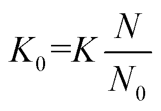 | (2) |
 | (3) |
Simply put, eqn (3) indicates that increasing the field strength induces greater acceleration of the ion, whereas increasing the particle density (i.e., the pressure) increases the collision frequency such that the time for acceleration becomes shorter. Ultimately, this interdependency indicates that the reduced field strength is directly proportional to the mean collision energy of any ion-neutral collision.7
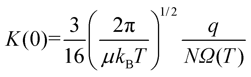
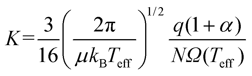
Within the low-field regime,7 an ion's velocity responds linearly to changes in the reduced field strength, and thus, enables relation of an ion's low-field mobility coefficient, K(0), to its collision cross section (CCS) via the Mason–Schamp equation (eqn (4)),8 whose derivation dates back to the early work on ion mobility by Langevin.9
 | (4) |
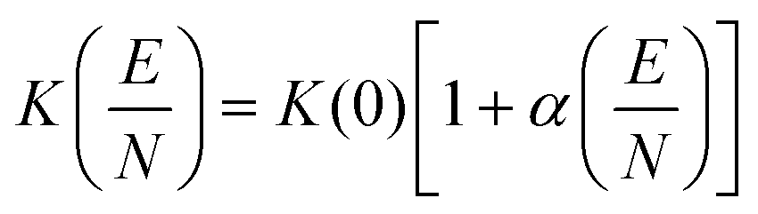
Here, μ is the reduced mass of the ion-neutral pair, kB is Boltzmann's constant, T is the absolute temperature of the bath gas, q is the absolute charge of the ion and Ω is the CCS. The CCS represents the orientally-averaged collision area of the analyte with the buffer gas that fills the mobility cell, and as such, is intrinsically related to the 3D structure of the ion. The ability of IMS to discern molecular geometric structure from an ion's CCS depends on two crucial factors: (1) the precise measurement of ion mobility under strictly controlled experimental conditions (i.e., temperature and pressure within the mobility region),4,10 and (2) the meticulous modeling of CCS/ion mobility from the computed geometry of the analyte. Owing to the significant role CCSs play in chemical separations, modelling CCS has become an integral component of IMS research. Calculating an ion's CCS in silico often mitigates ambiguity in IMS-based structural assignments and provides valuable insight into the nature of the IMS-based separation mechanism.11 When modeling ion mobility, practitioners are primarily concerned with capturing the dynamics of a collision event between an ion and a gas particle, as collisions strongly depend on the electric field, pressure, and temperature. To express this relationship, the ion mobility is adjusted by the alpha function, which is usually expressed as a Taylor series composed of even-ordered alpha coefficients (α2n; eqn (5a) and (5b), respectively).12
 | (5a) |
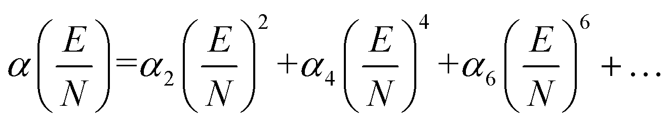 | (5b) |
The alpha function is approximately zero if the reduced field strength is within the so-called low-field limit (ca. 0–10 Td), which is why low-field IMS techniques such as drift-tube IMS (DT-IMS) can be used as a tool for both structural elucidation and analytical separations. Structural elucidation is typically performed within the low-field limit, where an ion's velocity distribution is characterized by a Maxwell–Boltzmann distribution at the temperature of the bath gas (T), and hence, renders the Mason–Schamp relation valid.
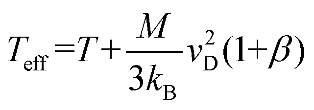
While advances in instrumentation have enabled high-throughput measurements of CCS on many low-field IMS platforms,11,13–16 development of computational frameworks for relating an ion's structure to its CCS has progressed at a much slower pace. Several methods (and software that implements these methods) have been published over the years to calculate CCSs, a summary of which is provided in the ESI (section S1†) and in ref. 17. However, most of the common CCS packages are limited to calculating thermal CCSs and/or low-field mobilities, and unfortunately are falling behind the surge in popularity of IMS techniques that operate at high field strengths.18,19 Both MobCal-MPI20 and IMoS21,22 are notable exceptions, as they have been modified to allow calculations of ion mobility at arbitrary field strengths. The calculation of mobilities above the low-field limit is based on the work of Kihara,23 Mason and Schamp,8 and Viehland and Mason,24,25 the latter of whom devised two-temperature theory (2TT) to account for the non-negligible acceleration of ions in electric fields that surpass the low-field limit. Viehland and Mason define an effective temperature (Teff) that is composed of thermal and field-induced contributions that describe the relative velocity distribution of the ion-neutral pair, which, when incorporated into eqn (5), generates eqn (6).24,25
 | (6) |
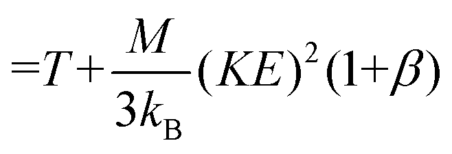
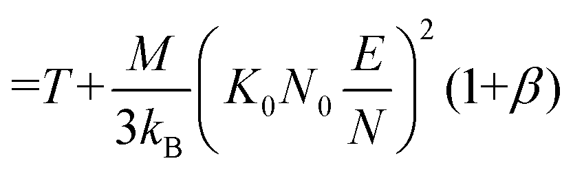
Note that Teff can be expressed in terms of the drift velocity (eqn (7a)), mobility coefficient (eqn (7b)), or reduced mobility coefficient (eqn (7c)), where M represents the molecular mass of the bath gas particle (i.e., 28 Da for N2).
 | (7a) |
 | (7b) |
 | (7c) |
Eqn (6) and (7) feature two correction factors, α and β, the former of which is distinct from the alpha function shown in eqn (5). These correction factors are non-zero when higher order approximations of 2TT are implemented but always result in an ion's Teff being greater than T for any field strength greater than 0 Td. However, for low-field conditions (ca. <10 Td), the contribution of the electric field to an ion's drift velocity is negligible, resulting in a relative velocity distribution of the ion-neutral pair that resembles its thermal velocity. Consequently, under low-field conditions Teff and T are equal, and eqn (6) simplifies to eqn (4). It is worthwhile to mention that modelling ion mobilities at arbitrary field strengths can be further improved by using three temperature theory (3TT)26,27 or the Gram–Charlier (GC) approach.28 However, due to their computational complexity, these methods are not commonly employed within the ion mobility community.
Despite our prior success in implementing the 2TT approach in modelling mobilities above the low-field limit,20 we have yet to formalize our approach within the IMS literature. Here, we report on an update to the parallelized CCS calculation suite MobCal-MPI, which is now capable of accurate ion mobility calculations at arbitrary field strengths. This update also optimizes the treatment of ion-neutral collisions with N2, where evaluating the ion-neutral interaction potential from both nitrogen atoms of N2 instead of its centre of mass results in more accurate CCS calculations. By coupling the updated treatment of ion-neutral collisions with an empirically corrected 2TT implementation, MobCal-MPI 2.0 enables precise and efficient calculations of high-field mobilities that accurately reproduce ion behaviour on high-field IMS platforms.
Methods
Modelling an ion's 3D structure and partial charges
Similar to its predecessor, MobCal-MPI 2.0 computes CCSs based on the ion's geometric structure given as xyz-coordinates, partial charges, and atom classes defined by the MMFF94 force field.29,30 In order to evaluate accuracy and calculation efficiency, we employ four different test sets: the calibration set (N = 162), validation set (N = 50), high-field validation set (N = 132), and peptide set (N = 12). The calibration and validation sets are composed of analytes with known CCSs (obtained from ref. 15, 16, 31–38), which encompass each atom type defined by the MMFF94 forcefield. Multiple conformers are considered for each analyte, which were obtained using the protocol outlined in the original MobCal-MPI publication.39 The high-field validation set is composed of small, rigid analytes (with a maximum of five conformers), for which our group has previously measured high-field mobility data.20,40,41 Finally, structures in the peptide set were generated from the lowest energy structure determined from their amino acid sequence using the I-TASSER suite,42,43 and are used exclusively for benchmarking. The peptide set contains 12 species ranging in length from 9 to 22 amino acid residues. To remove ambiguity in charge site assignment, the N-terminus and all basic residues (i.e., His, Lys, and Arg) of each peptide were protonated, leading to charge states ranging from +2 to +5.All structures in the calibration, validation and high-field validation sets were reoptimized using density functional theory (DFT) at the ωB97X-D3/def2-TZVPP level of theory.44–48 Subsequent calculation of partition functions (via computation of vibrational frequencies and rotational constants) at the same level of theory enables Boltzmann weighting of different conformers for each ion. Atomic partial charges were computed via the CHELPG partition scheme using a grid composed of points spaced apart by 0.1 Å, where each grid point is at most 3.0 Å away from any atom in the molecule.49 Due to the size of the molecules within the peptide set, calculations were conducted using the faster TPSS-D3/def2-TZVPP level of theory50 and a coarser grid for partial charges (0.3 Å spacing, 2.8 Å cut-off). DFT optimization of the structures obtained from I-TASSER was not necessary as the peptide set merely served for benchmarking. All DFT calculations were conducted with the ORCA 5.0.3 program suite51,52 and were uploaded to the ioChem-BD database53,54 (see https://iochem-bd.bsc.es/browse/review-collection/100/285126/7ae31bce0ab75f49f8043e51). Subsequent determination of the MMFF94 force field atom types was undertaken using OpenBabel.55 We note that the level of theory chosen for the DFT calculations can influence the subsequent CCS calculations through the accuracy of determining the ion structure (bond lengths and angles), the atomic partial charges, and the thermochemistry in case a Boltzmann weighting scheme is used to weight the CCS of multiple conformers. A systematic investigation of the performance of different basis sets and functionals has been conducted before with MobCal-MPI.56 It was found that the performance was comparable between different hybrid functionals in conjunction with double or triple zeta basis sets augmented with polarization basis functions. We expect that MobCal-MPI 2.0 can be employed for structures determined using several model chemistries, although for consistency, we recommend users conduct geometry optimizations and evaluate thermochemistry using the methods employed for the calibration and validation sets (ωB97X-D3/def2-TZVPP).
Evaluating collision integrals using the Chapman–Enskog formalism
The motion of ions through a gas is governed by the Boltzmann transport equation.57 The quantity of interest in this framework is the ion velocity distribution, fion. One can calculate the drift velocity (vD) as a moment of the ion velocity distribution (fion; eqn (8)), for which we use the convention that the electric field points along the z-axis. Note that n is a normalization factor.7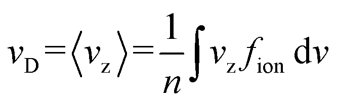 | (8) |
Although the velocity distribution of the bath gas particles (fbg) can be described by a Maxwell–Boltzmann distribution at temperature T, fion will be distorted compared to fbg due to the acceleration caused by the electric field. Within the framework of 2TT, field-induced acceleration of the ion is accommodated by introducing a second temperature (Tion) that accounts for the skewed velocity distribution. The effective temperature described in eqn (7) reflects the distribution of relative velocities between bath gas particles and ions. In general, Tion ≥ Teff ≥ T.
To solve for fion, one can apply the Chapman–Enskog formalism,58,59 which expresses fion as a Taylor series of basis functions. 2TT expands on this formalism by using Burnett-like basis functions, which are defined in eqn (9a) and (9b):24,25
| ψ(r)lm(wion) = wlionS(r)l+1/2(w2ion)Yml (θ,ϕ) | (9a) |
| w2ion = mv2/2kBTion | (9b) |
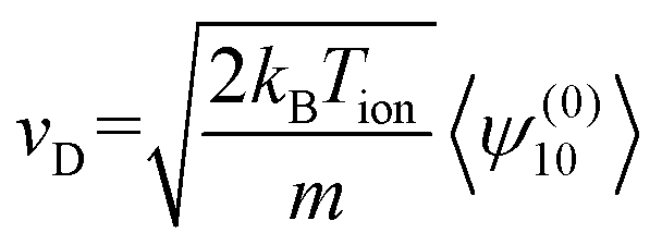
Here, S(r)l+1/2 are Laguerre polynomials, Yml are the spherical harmonics, m is the molecular mass of the ion, and v is its velocity. wion acts as dimensionless velocity to simplify the equations. Rather than solving for the full ion velocity distribution, 2TT attempts to find solutions only to the moments of these basis functions. This is sufficient for ion mobility because the drift velocity can be expressed as moment of ψ(0)10, as per eqn (10).
 | (10) |
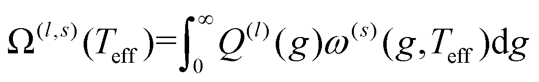
Iterative computation is used to solve for these moments, with higher-order approximations requiring additional iterations. The specifics of the iterative procedure are beyond the scope of this manuscript, although interested readers are directed to ref. 24 and 25 for further information. Within this formalism, the matrix elements ars(l) appear, which can be expressed as linear combinations of irreducible collision integrals, Ω(l,s). For simplicity, we report the form of the Ω(l,s) only for spherically symmetric ion-neutral interaction potentials in eqn (11a)–(11c).
 | (11a) |
 | (11b) |
 | (11c) |
Here, b is the impact parameter, g is the relative velocity between the collision partners, χ is the scattering angle of the collision event (see Fig. 1), and Q(l) are the momentum transfer integrals. Note that the collision integrals (Ω(l,s)) depend on Teff since it is this temperature that describes the collision dynamics between ions and neutrals. In the first order approximation of 2TT, eqn (6) can be solved by computing solely Ω(1,1) since α = 0. However, MobCal-MPI 2.0 employs the 2nd order approximation of 2TT, which requires calculating collision integrals up to Ω(2,4) so that all necessary matrix elements (i.e, ars(l)) can be derived. The linear combinations needed to obtain the ars(l) from the Ω(l,s) are tabulated for 2nd order 2TT,7 and were hard coded into MobCal-MPI 2.0. It should be noted that the relationship between the ars(l) and Ω(l,s) can also be obtained algorithmically if higher order approximations are desired,25,60 although our research has indicated that 3rd order 2TT provides only a slight improvement in the accuracy of mobility calculations compared to 2nd order 2TT for the systems typically studied in IMS.20
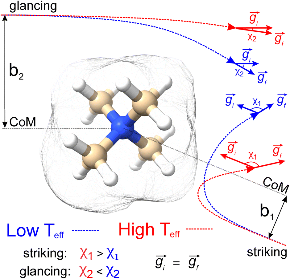 | ||
| Fig. 1 Schematic representation of how the trajectory method is employed for CCS calculations, using NMe4+ as an example. Two collision events are shown (striking vs. glancing) that exhibit different impact parameters (bstriking < bglancing) and relative velocities (gblue < gred), the latter of which corresponds to differing effective temperatures (higher Teff is associated with higher g). The scattering angle, χ, is calculated from the angle between the initial and final velocity vectors. Note that ion-neutral collisions are treated elastically, so the remission velocity (gf) is equivalent to the incident velocity (gi). Isosurfaces correspond to the envelope of vdW radii of the atoms contained within the molecule. | ||
Sampling collision events using the trajectory method
Fig. 1 shows a schematic depicting the general methodology of the trajectory method (TM) to compute collision integrals. Importantly, the collision dynamics must be sampled to evaluate the scattering angle (χ), which depends on three variables: the relative velocity of the ion-neutral pair (g), the impact parameter (b), and the orientation of the ion relative to the starting position of the collision partner (N2). Evaluation of χ requires simulation of the trajectory that the buffer gas takes upon colliding with the analyte. Depending on the initial conditions (i.e., g, b, and ion-neutral orientation), substantially different collision behaviour can be observed. For example, N2 will be scattered to a much greater extent for collisions defined by a small impact parameter (striking collision) compared to a large impact parameter (glancing collision). In terms of the relative velocity of the ion-neutral pair, which is determined by the effective temperature, the degree of scattering diminishes for glancing collisions with increasing g. In contrast, the relative velocity has a significantly smaller impact on χ for striking collisions (see Fig. S1†). After remission of the gas molecule, χ is calculated as the angle between the initial and final vectors that define the trajectory of the buffer gas, the magnitude of which are equal because MobCal-MPI 2.0 treats collisions elastically. With χ in hand for all starting conditions sampled, the CCS can be obtained via integration as per eqn (11).Within eqn (11), integration over b and the orientation of the ion (eqn (11c)) is accomplished using Monte–Carlo (MC) sampling. In other words, the ion is randomly rotated in space and an impact parameter is randomly chosen between 0 and an initially derived bmax (see section S3 of the ESI† for details). The sample size of this MC integration is termed imp in MobCal-MPI. In contrast, the integration over the relative velocity of the ion-neutral pair is sampled on fixed grid points, which are denoted inp. In the previous implementation of MobCal-MPI, a weighted grid was used to efficiently integrate over velocity space (eqn (11a)).39,61,62 However, changing the temperature that defines the velocity distribution requires the weighted grid to be modified for every collision integral because the weighting functions (ω(s)) depend on s and Teff (as per eqn (11b)). Since our goal is to efficiently calculate multiple collision integrals (up to Ω(2,4)) over the range defined by the temperature of the bath gas (T) and the highest effective temperature desired by the user (Teff,max), we implemented a linear grid of velocity points defined by the temperature range. Because the linear grid of velocities is shared between all CCS integrations, only one set of N2 scattering trajectories is required to evaluate all collision integrals. In other words, using a linear grid to sample collision events between T and Teff,max enables the simultaneous evaluation of the ion's mobility and CCS at any temperature within this range.
Statistical analysis of the sampled collision events
The integration over the MC sampled trajectories for a fixed relative velocity (g) yields the momentum transfer integrals (Q(l)) for that particular velocity. To estimate the statistical uncertainties associated with the sampling, the integration is repeated itn times (yielding Q(l)i(g) for i = 1, …, ith), which in turn produces an average, standard deviation, and confidence interval (CI) according to eqn (12a), (12b), and (12c), respectively. | (12a) |
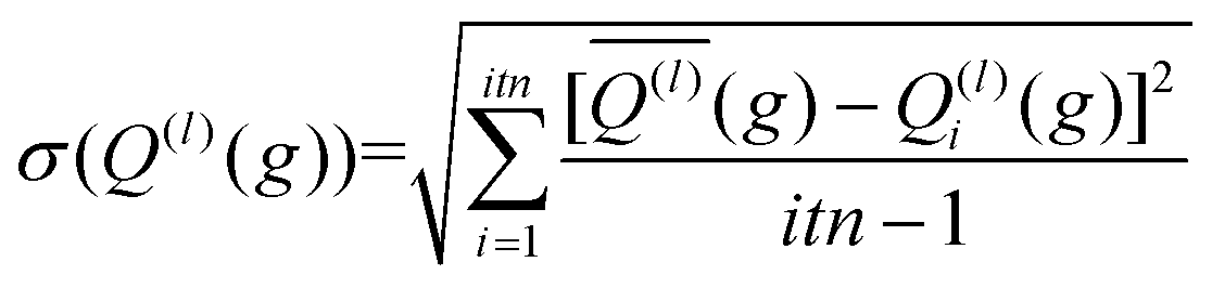 | (12b) |
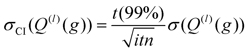 | (12c) |
Here, t (99%) = 2.57 is the two-sided, 99% quantile of the standard normal distribution. Increasing the amount of MC sampling points (imp) will lower the variances of the Q(l)i(g), and increasing the number of repetitions (itn) will increase confidence in the average. Consequently, both values affect the uncertainty, which is represented by the 99% confidence interval.
The above analysis is performed for each point within the velocity grid, which has a size of inp. The momentum transfer integrals are then integrated over these velocity grid points to yield the collision integrals (eqn (11a)). This integration can also be viewed as taking a weighted average of the Q(l)(g), whereby ω(s)(g) reflects the weighting function. Thus, the uncertainties associated with each Q(l)(g) can be propagated according to eqn (13), where Δg is the spacing of the velocity grid.
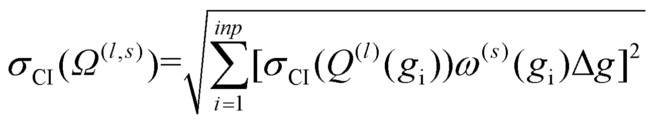 | (13) |
Increasing inp decreases Δg, and hence, decreases the uncertainty of the calculated CCS. Given that Ω(1,1) is the primary contributor to the mobility for all field strengths, and that other Ω(l,s) provide only small corrections, we consider only σCI(Ω(1,1)) when evaluating the uncertainty of the mobility coefficient (K). It is worth noting that eqn (13) does not require an additional normalization factor, as 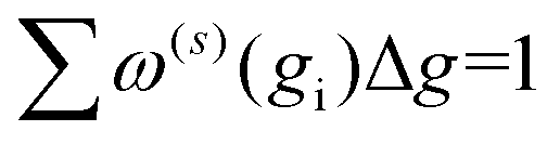 .
.
Evaluating high-field mobilities via 2TT
To calculate high-field mobilities, the user is prompted to give a range of effective temperatures, whereby the lowest temperature (T) is equivalent to the bath gas temperature of their IMS instrument, and the highest temperature (Teff,max) denotes the maximum effective temperature for which they wish to compute mobilities. The velocity grid is set up accordingly, and the momentum transfer integrals are computed for each velocity grid point. Then, for a given Teff,i, all required collision integrals Ω(l,s) and matrix elements ars(l) are computed. Next, the truncation-iteration procedure from 2TT theory is used to calculate the required moments 〈ψ(r)lm〉 using the 2nd order approximation.20,25 From this, the drift velocity (cf.eqn (10)) and the reduced field strength are obtained, whose ratio yields the ion mobility coefficient as per eqn (3). Due to the quadratic relationship between Teff and E/N (cf.eqn (7)), the distribution of E/N values obtained from the linear grid of effective temperatures is non-uniform, with a greater density of grid points at higher field strengths. Fortunately, the ion mobility coefficient exhibits larger changes as the field strength increases, so the denser sampling of points at higher E/N enables more accurate reproduction of its behaviour.Results and discussion
Optimizing the accuracy of CCS calculations
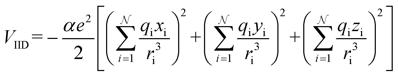
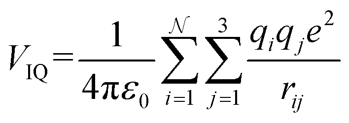
In MobCal-MPI 2.0, we retain the form of the ion-neutral interaction potential (Vtotal) from its predecessor, which consists of a van der Waals (vdW) term composed of a modified Buckingham potential (Exp-6) used in the MM3 forcefield (VvdW; eqn (14a)),63 an ion-induced dipole term (VIID; eqn (14b)), and an ion-quadrupole term (VIQ; eqn (14c)).39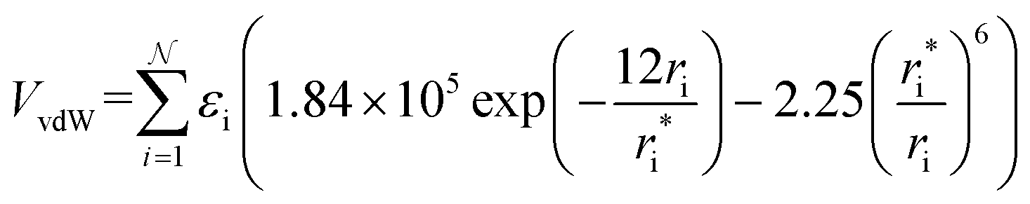 | (14a) |
 | (14b) |
 | (14c) |
| Vtotal = VvdW + VIID + VIQ | (14d) |
With increasing buffer gas polarizability, the VIID term plays an increasingly significant role in the ion-neutral potential. If the buffer gas possesses a quadrupole moment (e.g., N2), the addition of an ion-quadrupole potential is crucial for the evaluation of accurate scattering trajectories.64,65 To effectively mimic the quadrupole moment of molecular nitrogen (4.65 ± 0.08 × 10−40 C cm2),66 partial charges of −0.4825e are assigned to each nitrogen atom and balanced by a point charge of +0.965e at its centre of mass. This simplifies the calculation of the ion-quadrupole potential using eqn (14c), where the atomic partial charges on the analyte (qi) are iterated over their distance to each pseudo charge-site of N2.
In the original MobCal-MPI publication,39 the εi and  parameters were based on the implementation from the Kim group,34 who combined atomic parameters from the MMFF94 force field for the ion with parameters for molecular N2.29,30 The enhanced accuracy of this approach can be attributed to the distinction of atom types within the MMFF94 framework (e.g., sp3versus sp2 hybridized carbon centres have different εi and
  ), allowing for the more accurate evaluations of the vdW component of the ion-neutral interaction potential. Because the MMFF94 parameters derived for N2 describe a molecular entity (i.e., diatomic nitrogen), the distance term in the VvdW pairwise interactions (ri) can be evaluated in two ways (Fig. 2). In the first case, N2 can be treated as pseudo atomic entity, whereby pairwise interactions are calculated with respect to its centre of mass (CoM). Alternatively, ion-neutral interaction potentials can be evaluated by considering the pairwise interaction between each atom in the analyte and each nitrogen atom in N2, and then averaging the result (Avg-N2). The latter case seems to be more reasonable, especially at short ion-neutral distances where the orientation of the N2 molecule significantly impacts the repulsive portion of the interaction potential (see Fig. S3†).
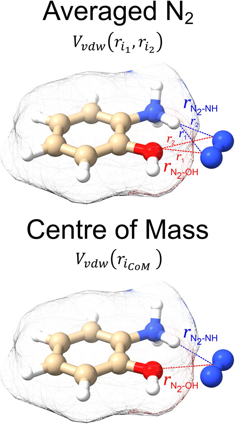 | ||
| Fig. 2 The two variations of calculating interaction potentials with N2 depicted for N-protonated 2-aminophenol. In the averaged N2 version, the potential is calculated from each atom of the ion to both atoms of N2, and subsequently averaged. In the centre of mass version, the potential is calculated from each atom of the ion to the centre of mass of the N2. Isosurfaces correspond to the envelope of vdW radii of the atoms contained within the molecule. | ||
Owing to the inherent parameterization of vdW terms within the MMFF94 forcefield, linear scaling parameters (ρdist and ρener) could be applied uniformly to the εi and  corresponding to each atom type, greatly simplifying their optimization (eqn (15a) and (15b)). This suggests that the same optimization methodology for ρdist and ρener can be applied to either the CoM or Avg-N2 version of the potential.
 | (15a) |
| ε′i = ρener·εi | (15b) |
To assess the accuracy of both the CoM and Avg-N2 approaches, we calculated the CCS of the 162 compounds in the calibration set using various combinations of ρdist and ρener, and compared the results with their experimentally measured CCSs obtained from ref. 15, 16, 31–38. Fig. 3A and B show the root mean square errors (RMSE) between the calculated and measured CCSs as contour plots for the Avg-N2 and CoM approaches, respectively. Similar to the previous version of MobCal-MPI, there is no single set of scaling parameters that performs best for MobCal-MPI 2.0, but rather a range of values that yield RMSEs of <2.5%. Interestingly, the CoM and Avg-N2 methods exhibit comparable accuracies despite the Avg-N2 approach being more physically realistic. It is possible that the similar accuracies observed for both approaches stem from the flexibility of the optimization of ρdist and ρener when only considering a finite set of test molecules. To validate the accuracy of both approaches, we selected a set of scaling parameters that performed well for the CoM (ρdist = 1.000 and ρener = 0.580) and Avg-N2 approaches (ρdist = 0.825 and ρener = 1.275), and assessed their accuracy using a separate set of 50 molecules (validation set; Fig. 3C and D, respectively).
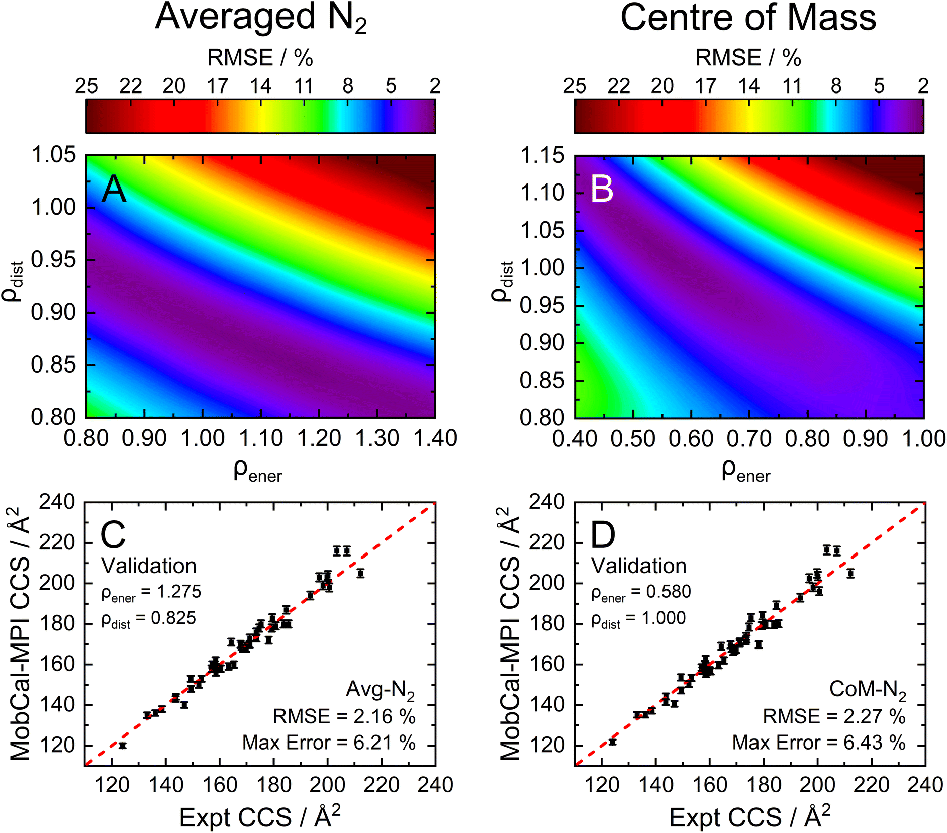 | ||
| Fig. 3 The RMSE, shown as a contour plot, for the optimization of ρdist and ρener using the (A) Avg-N2 or (B) CoM approach for the calibration set (162 molecules). To validate the accuracy of (C) Avg-N2 or (D) CoM approaches, we employed the values of ρdist and ρener yielding the lowest RMSE to calculate the CCS of 50 distinct molecules that were not present in the calibration set (validation set). All CCS calculations were performed at 298 K with itn = 5, inp = 104, and imp = 512. | ||
By examining the differences between the experimentally determined and calculated CCSs of the validation set, it can be concluded that the Avg-N2 and CoM methods both produce accurate results. We were surprised to find that the RMSE of the CoM version (2.27%) is only slightly larger than the RMSE of the Avg-N2 approach (2.16%). The reason for their similarity is likely due to the prevalence of glancing collisions at 298 K, which account for approximately 75% of all collisions for a molecules with a CCS of 160 Å2.20,67 The CoM approach, which does not accurately capture the repulsive portion of the interaction potential (Fig. S3†), still produces accurate CCSs at room temperature because the repulsive portion is only important when evaluating striking collisions. However, usage of the CoM rather than the Avg-N2 approach is not justified at high reduced field strengths because an inaccurate treatment of ion-neutral repulsion will result in erroneous CCSs under conditions where striking collisions dominate (i.e., at high Teff). For this reason, we implemented the Avg-N2 approach in MobCal-MPI 2.0. We expect the Avg-N2 approach will ensure greater internal consistency of the code when adding other collision gases (e.g., CO2, SF6), for which an explicit treatment of all atoms will be important.
Assessing CCS calculation uncertainty via the statistical analysis of collision events
After optimizing the scaling parameters for the Avg-N2 approach, we assessed the ability of our new method to propagate statistical uncertainties that determine the uncertainty of CCS calculations. In the previous version of MobCal-MPI, the uncertainty in a CCS calculation was determined by the standard deviation in the CCS measured during each itn mobility cycle. While this methodology does assess uncertainty in a reasonable manner, it does not explicitly consider the effects of all integration parameters on the final uncertainty (i.e., itn, imp, and inp). Our new methodology for treating uncertainty is depicted in Fig. 4 using protonated caffeine as an example. Here, the standard deviation in the calculated momentum transfer cross sections (Q(l); panel A) and the integrand for the CCS (Q(l)ω(s); panel B) are shown as a function of the relative velocity (g). Because we only sample a finite number (imp) of randomized trajectories per velocity point, the individual Q(l)i(g) for each itn will be slightly different, the standard deviation of which is shown by the shaded areas in Fig. 4A. The confidence interval describes that the value of Q(l)(g) upon infinite sampling of trajectories (i.e., the statistically “true” value) lies within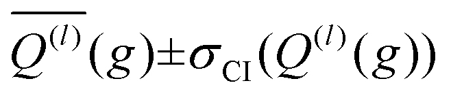 with 99% confidence (cf.eqn (12c)); this value is reported in the output of MobCal-MPI 2.0. Thus, increasing the number of trajectories sampled (imp) reduces the standard deviation, while increasing the number of iteration cycles (itn) reduces the uncertainty with respect to the “true value”. Further, increasing the number of velocity points (inp) yields a finer grid along the x-axis, which in turn increases the accuracy of the numerical integration, and leads to a decrease in the final uncertainty of the collision integrals, σCI(Ω(l,s)).
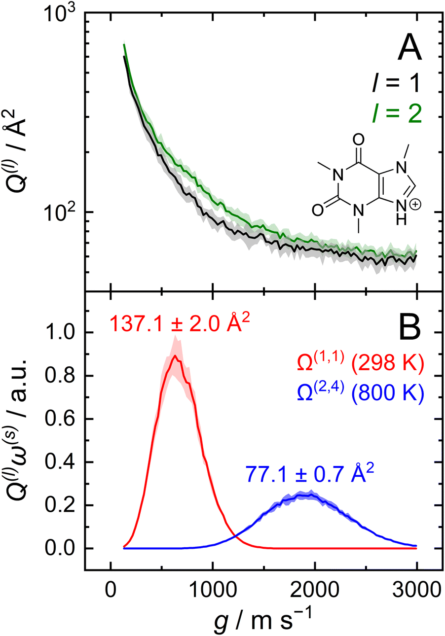 | ||
| Fig. 4 (A) Momentum transfer integrals and (B) CCS integrands of protonated caffeine. The standard deviations from eqn (12b) are shown as shaded areas, and the final uncertainty for Ω(l,s) corresponds to that from eqn (13). CCS calculations were performed using itn = 10, inp = 104, imp = 512 and T = 298 K (panel B; red) for Ω(1,1), and Teff,max = 800 K for Ω(2,4) (panel B; blue). | ||
In this statistical analysis, we observe a general trend where collision integrals of higher order (i.e., s) or at higher temperatures always exhibit smaller uncertainties. For example, Fig. 4A shows that the degree of momentum transfer decreases as the relative velocity between collision gas and ion increases. This decrease occurs because the contribution of glancing collisions to the total momentum transfer continually decreases with g until all collision events are striking (see Fig. S2†).59 Consequently, the standard deviations σ(Q(l)) also decrease with g, leading to differing uncertainties for the two collision integrals shown in Fig. 4B (2.0 Å2vs. 0.7 Å2). This disparity is a consequence of the respective weight functions (ω(s)), which are centred at different relative velocities owing to their evaluation at distinct values of s and Teff. Note that the functional dependency of Q(l) on g is influenced by the various terms in the interaction potential.68
Although the decrease in CCS uncertainty with increasing temperature cannot be avoided unless a weighted grid for g is used, our implementation of the linear grid enables the near-instantaneous evaluation of an ion's CCS for any temperature within a user-specified range once the Q(l) are determined. This occurs because an ion's CCS is determined from the area under the curve of Q(l)ω(s), the calculation time for which is practically instantaneous compared to the time required to evaluate N2 scattering trajectories from ∼106 collision events. However, accurate numerical integration necessitates that Q(l)ω(s) goes to zero as it approaches the integration limits. To ensure this condition is met, we establish integration boundaries encompassing the relative velocities that contribute to collision integrals at a given Teff. Fig. 4B illustrates this process, where the lowest order collision integral (Ω(1,1)) evaluated at the lowest temperature specified by the user (i.e., T) determines the lower velocity integration limit. Similarly, the highest-order collision integral (Ω(2,4)) evaluated at the highest user-specified effective temperature (i.e., Teff,max) establishes the upper velocity integration limit. The exact method for determining integration limits using Q(1)ω(1) and Q(2)ω(4) is provided in the ESI (section S2†). Since the upper and lower limits of the effective temperature determine the range of relative velocities sampled, assessing trajectories on a common velocity grid produces internally consistent Q(l). This enables the use of the same trajectories to evaluate Q(l)ω(s) at any temperature between T and Teff,max, thereby enabling straightforward determination of any CCS within the temperature range via numerical integration. By implementing the linear grid, MobCal-MPI 2.0 offers significantly faster CCS calculations for multiple temperatures compared to its predecessor, where collision integrals had to be recalculated for each user-specified temperature. In other words, if a user wants to compute CCSs at n effective temperatures, calculation via the original MobCal-MPI code would take n-times longer compared to MobCal-MPI 2.0.
An in-depth analysis of the uncertainty in CCS calculations
Owing to the impact of the size of inp and imp on the final uncertainty of calculated CCSs, a comprehensive analysis is required to understand their exact effect. This was accomplished by calculating the CCSs (T = 298 K) of the validation set using discrete sampling sizes for the impact parameter (imp; 256, 512, 768, and 1024) and the relative velocity of the ion-neutral pair (inp; 56, 104, 152, and 200). For optimal CCS calculation efficiency within the parallelized framework of MobCal-MPI 2.0, sampling sizes for inp and imp were chosen to be divisible by the number of cores used for the CCS calculation (here, Ncores = 8). The distribution of final relative uncertainties (σCI(Ω(1,1))/Ω(1,1)) is shown as a violin plot for each (imp,inp) combination, with the mean relative uncertainty noted in blue (Fig. 5). As expected, the relative uncertainty decreases as the number of sampling points in either the imp or inp dimension increases. The average computing time also increases with increasing imp and inp because the number of trajectories sampled during one itn cycle is given by the product of imp and inp.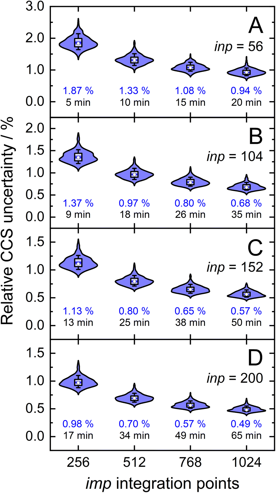 | ||
| Fig. 5 Distributions of relative CCS uncertainties, σCI(Ω(1,1))/Ω(1,1), for the validation set (N = 50) for different combinations of velocity sample points (inp) and orientation/impact parameter sample points (imp). Blue numbers below each distribution correspond to mean relative CCS uncertainties and black numbers to average computing time. | ||
Our statistical analysis of uncertainty indicates the presence of a partial invariance along the diagonals of Fig. 5. For example, the mean relative uncertainty and calculation time for (imp,inp) = (768,104) is similar to that observed from the (imp,inp) = (512,152) set. Using these relatively large inp grid sizes was necessary because of the changes implemented to MobCal-MPI 2.0, whereby velocities are sampled using a linear grid. Compared to its predecessors,61,62 which used a weighted velocity grid that confined the velocity distribution to values populated at the temperature of the CCS calculation, only 48 inp points were required to achieve a mean relative uncertainty of 0.95%.39 However, since the linear grid does not confine the velocity distribution to values populated at the effective temperature of the CCS calculation, additional velocity points are necessary to achieve an equivalent level of precision. Consequently, users should choose a set of (imp, inp) such that: (1) the statistical uncertainty of MobCal-MPI 2.0 parallels that of its predecessor, and (2) the statistical uncertainty does not exceed the RMSE between calculated and experimental CCS (2.16%; cf. Fig. 3B). We recommend settings of imp = 512 and inp = 104 for routine CCS evaluations, e.g., when different analytes in an IMS spectrum are well separated, as this offers a balance between good precision and calculation time. If higher precision is desired, e.g., when two isomers or protomers with very similar CCS are to be distinguished, we recommend settings of imp = 768 or imp = 1024 in tandem with an inp setting of 200 (Table 1). This should allow for a confident assignment of closely eluting species, even if there is a systematic deviation caused by the underlying DFT calculations.
| Calculation type | Parameter | ||
|---|---|---|---|
| itn | inp | imp | |
| Routine | 10 | 104 | 512 |
| High-precision | 10 | 200 | 768 or 1024 |
We would like to remind readers that the uncertainties shown in Fig. 5 are not reflective of the deviation between an experimentally measured and calculated CCS, but rather pertain to the uncertainties in the statistical sampling of collisions and how this uncertainty is propagated within the computational workflow. Moreover, the statistical uncertainties of the CCSs depend on the range of effective temperatures used in the calculation. Fig. 4B illustrates that for a considerable fraction of the velocity grid points, Q(l)ω(s) values become negligible when the upper end of the velocity grid is defined by a relatively high effective temperature (i.e., Teff,max ≫ T), thereby negating their contribution to the CCS integrand at high Teff. To evaluate the effect of grid sizes on CCS calculations performed for a range of effective temperatures, we undertook an analysis akin to that of Fig. 5. In this case, the relative uncertainty for CCSs when evaluated between T = 298 K and Teff,max = 800 K are approximately 30% larger than those for a CCS calculation performed solely at T = 298 K (1.26% vs. 0.97%; see Fig. S4†). Because this comparison was made for the suggested sampling sizes of inp = 104 and imp = 512, we recommend that users seeking CCSs at various effective temperatures employ the high-precision sampling sizes. For T = 298 K and Teff,max = 800 K, inp = 200 and imp = 1024 yields a mean relative uncertainty of 0.64% for Ω(1,1) at T = 298 K, which decreases further for the higher temperatures. Despite the high-precision settings being more computationally expensive, the linear grid significantly decreases the computing time because the trajectories determining the Q(l) need be evaluated only once. Thus, the added computational expense is offset, making this drawback relatively minor in terms of the efficiency of MobCal-MPI 2.0.
Implementing 2TT within MobCal-MPI for mobility calculations at arbitrary fields
In the MobCal-MPI 2.0 interface, users are prompted to input the bath gas temperature and an upper limit for the ion effective temperature (i.e., T and Teff,max, respectively). Specifying a temperature range calls the 2TT module, which initiates calculation of the ion's CCS and reduced mobility at reduced field strengths that fall within the given temperature range. Users can also specify a grid size for the temperature range such that CCSs and reduced mobilities are printed at desired increments of Teff. Table 2 shows an example output from MobCal-MPI 2.0, where the CCS and reduced mobility of protonated amoxapine in N2 was calculated between T = 373 K and an arbitrary choice of Teff,max = 700 K on a temperature grid composed of 8 points. For brevity, we opted to remove the drift velocity from the printout, as this quantity is easily obtained from the reported data viaeqn (3). T = 373 K corresponds to the bath gas temperature, which yields a CCS and reduced mobility in the zero-field limit (i.e., E/N = 0). Because all collision integrals are evaluated on the same linear velocity grid, users can increase the number of points sampled within the temperature range up to Teff,max without incurring an increase in calculation time.| T eff/K | E/N/Td | K 0/cm2V−1 s−1 | CCS/Å2 | Uncertainty |
|---|---|---|---|---|
| 373.0 | 0.0 | 1.2250 | 154.27 | 0.64% |
| 402.7 | 50.0 | 1.2162 | 150.08 | 0.63% |
| 449.0 | 81.3 | 1.2028 | 144.50 | 0.62% |
| 501.8 | 107.9 | 1.1878 | 139.19 | 0.61% |
| 551.4 | 129.1 | 1.1742 | 135.02 | 0.61% |
| 600.9 | 148.2 | 1.1609 | 131.44 | 0.60% |
| 650.5 | 166.1 | 1.1479 | 128.34 | 0.59% |
| 700.0 | 183.0 | 1.1353 | 125.63 | 0.58% |
Notably, the CCS and its uncertainty decreases at higher effective temperatures, which is a consequence of the decreased efficiency in momentum transfer with increasing relative velocity (cf.Fig. 4).20,59,67,68 The inverse relationship between CCS and mobility leads one to expect that K0 should increase with Teff, but this is not the case. The decrease of K0 with Teff is a consequence of the kinetic theory of gases, which states that the apparent viscosity of the collision gas increases with Teff.69,70 This underscores the fact that the ion mobility is not a constant, but is rather a function of the field strength. Since the reduced field strength computed by MobCal-MPI 2.0 is determined by the effective temperature of the ion, the alpha function can be readily obtained from the calculated mobility data using eqn (16) and subsequently fit to an even order polynomial of the form given by eqn (5b) to determine the alpha coefficients. Employing this workflow for protonated amoxapine results in α2 = −2.935 × 10⁻⁶ Td−2, α4 = −3.080 × 10⁻¹¹ Td−4 and α6 = −2.553 × 10⁻¹⁶ Td−6.
 | (16) |
To assess the accuracy of 2TT in calculating high field mobilities, one can compare the alpha curves obtained through experimentation and computation. This comparison is shown in Fig. 6A for protonated amoxapine (blue trace), whose experimental alpha curve (black trace) was determined using the protocol outlined in section S7 of the ESI.† MobCal-MPI 2.0 captures the general trend of amoxapine's alpha curve, which adopts increasingly negative values as the reduced field strength increases. However, the computed alpha curve exhibits more negative values than the experimental curve, indicating that calculated mobility coefficient decreases faster with field strength compared to the actual measurement. This finding aligns with the observations made by Siems et al.,71 who reported that the 2TT approach yields accurate mobilities at low and medium field strengths, but underestimates mobilities at high field strengths. Consequently, alpha curves evaluated using 2TT will almost always exhibit a systematic, negative deviation, especially at high field strengths.
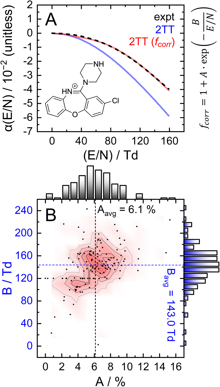 | ||
| Fig. 6 Investigation of the empirical correction to 2TT. (A) Comparison of experimental and calculated alpha functions for protonated amoxapine. Optimized parameters are A = 4.4% and B = 132 Td. (B) 2D distribution of optimized A and B parameters of the empirical correction, fcorr, over 132 test cases. | ||
To address the systematic deviation between the computed and measured alpha functions, we introduced an empirical correction to 2TT, inspired by the form of the deviations found by Siems et al. (see section S6 of the ESI† for details).71 Briefly, a field-dependent correction factor (fcorr) is used to adjust the mobilities calculated from 2TT (K2TT) using eqn (17).
| Kcorr = fcorr·K2TT | (17a) |
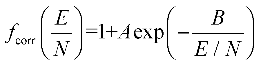 | (17b) |
The parameters A and B, which represent the maximum deviation at infinitely high field strengths and the field strength at which deviations become significant, respectively, can be tuned for a specific ion such that the deviation between the computed and measured alpha curves is minimized. For protonated amoxapine, optimizing A and B leads to almost perfect alignment of the computed and experimental alpha curves (Fig. 6A; red trace). Moreover, the value obtained for A (4.4%) is consistent with the range reported by Siems et al. (5–7%), and the value of B = 132 Td indicates that the correction becomes most significant at high field strengths.
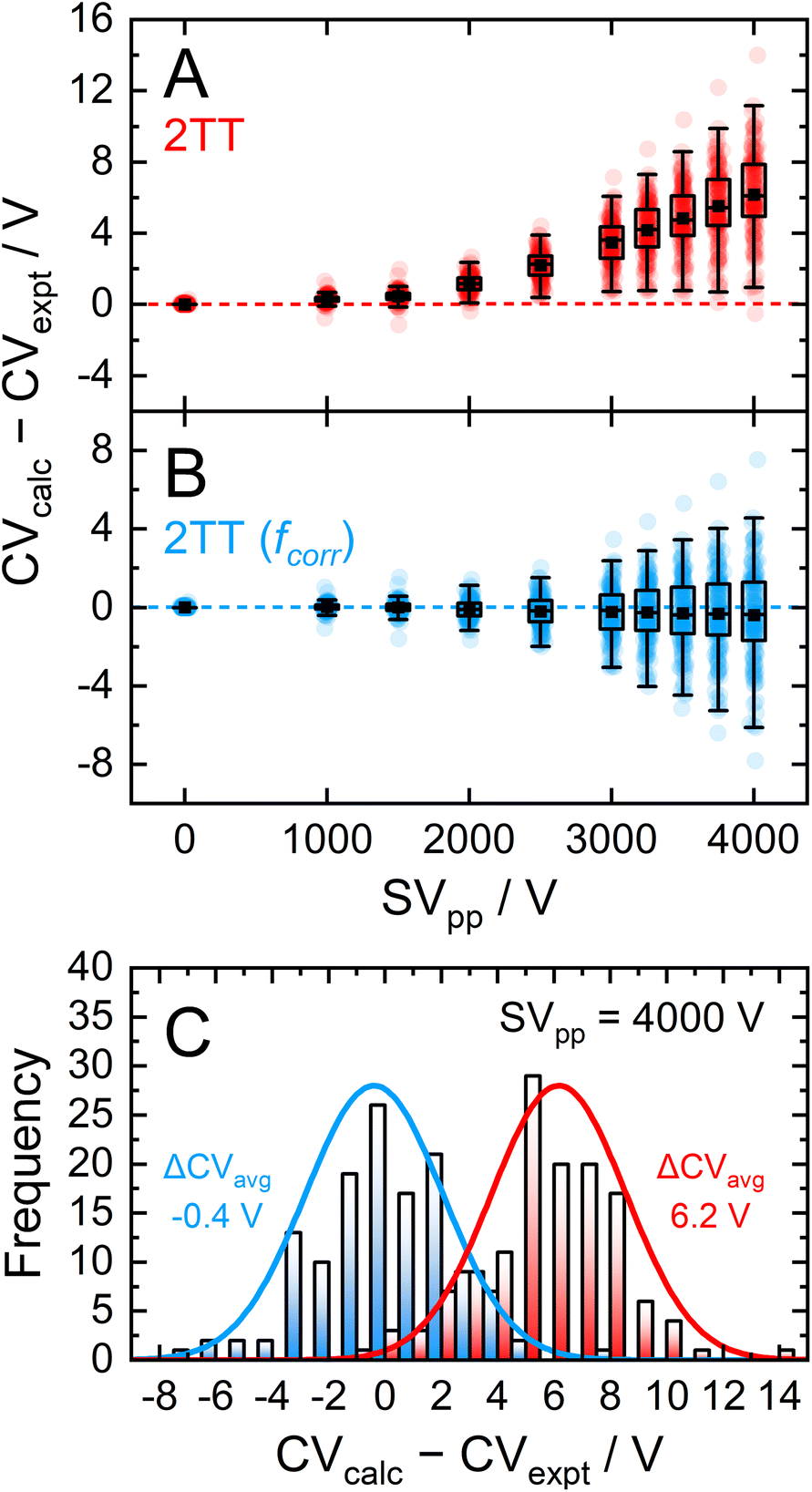
To investigate the general performance of the empirical correction, we assessed its ability to correct high-field mobilities for a large set of compounds. An efficient means of obtaining a dataset of high-field mobilities is via differential mobility spectrometry (DMS), which is also known as field-asymmetric ion mobility spectrometry (FAIMS).12,18,72 In DMS, the ions are subjected to an asymmetric waveform (separation voltage; SV) that consists of high-field and low-field components. The SV induces the off-axis displacement of the ion by an amount proportional to its alpha function. The application of a species-specific compensation voltage (CV) to the SV enables ions to traverse the DMS device; at a given SV, each analyte is transmitted at a distinct CV that is intrinsically linked to the ion's alpha function. By monitoring the dependence of the CV required for analyte transmission at different strengths of the SV field, the corresponding SV vs. CV relationship (i.e., a dispersion plot) can be employed to derive the alpha function using the method described in section S7 of the ESI.†12
Dispersion plots for 132 compounds were procured from previously published datasets from our group to generate the high-field validation set.20,40,41 Each analyte's dispersion plot was recorded on the SelexION DMS platform (SCIEX; 1 mm gap and T = 373 K) in a pure N2 environment between SV = 0–4000 V. In theory, each analyte's dispersion curve can be converted to the corresponding alpha curve using the methodology outline in section S7.† However, because our goal is to reproduce experimentally measured quantities, we employed an iterative method previously published by our group to calculate dispersion plots from the mobility data generated by the 2TT implementation within MobCal-MPI 2.0.73 In general, the calculated dispersion plots displayed positive compensation voltage (CV) shifts relative to those determined experimentally (Fig. 7A). Positive CV shifts indicate that the systematic underestimation observed for protonated amoxapine is also observed for most compounds in the high-field validation set.
 | ||
| Fig. 7 Comparison of measured vs. calculated dispersion plots over a range of separation field amplitudes as box plots for (A) uncorrected 2TT and (B) 2TT including the empirical correction employing Aavg and Bavg. Panel (C) shows the distribution of CV deviations using the uncorrected and empirically correct 2TT at the highest SVpp (4000 V). | ||
Since the empirical correction to 2TT could be employed to replicate the alpha curve of amoxapine, it is reasonable to assume that the same approach can be employed to address the systematic CV shift observed in the dispersion plots. To this end, A and B were optimized such that the deviation between the calculated and experimental dispersion curves was minimized (for select examples, see Fig. S7†). Fig. 6B shows the distributions of the A and B parameters obtained for each compound in the high-field validation set, the majority of which align with the results found by Siems et al. (5–7% for A and 100–200 Td for B).71 The parameters exhibit unimodal distributions when considered independently or together, the latter of which is best visualized in the contour plot. The data also suggests little to no correlation between the two parameters, although it is worth noting that B becomes undefined as A approaches zero.
Expanding the applicability of the empirical correction to various chemical systems necessitates knowledge of values for A and B a priori such that they can be applied to a broad range high-field mobilities predicted by 2TT. Because these parameters are uniformly distributed about their respective means and are seemingly uncorrelated with properties relevant to collision theory (see Fig. S8†), we chose to use the average values of A (6.1%) and B (143.0 Td) to test the accuracy of this approach. Aavg and Bavg were hard-coded into MobCal-MPI 2.0, enabling the calculation of high-field mobility data using a uniform set of correction factors. The deviations between calculated and experimental dispersion plots that either employ or exclude the empirical correction to 2TT are shown in Fig. 7. As previously mentioned, exclusion of the empirical correction results in a systematic overestimation of the CV values for all 132 species, especially at high field strength. Using the empirical correction with Aavg and Bavg removes the systematic deviation, shifting the average error in CV towards zero for all SVs sampled in the dispersion plot. Fig. 7C shows the distribution of CV deviations at SVpp = 4000 V. When applying the empirical correction, over 88% of the data falls within a ±4 V range of the experimental value. The mean deviation between calculated and experimental CV is −0.4 V at SV = 4000 V, equivalent to a relative deviation of approximately 4%. The full width at half maximum (FWHM) of this distribution is 5.7 V, which is comparable to the experimental FWHM at this separation field amplitude (≈3 V).18 It is worth mentioning that the variances are virtually unaffected by the empirical correction, meaning that this approach strictly corrects the general deviations of 2TT in determining high-field mobilities but does not impact uncertainties specific to individual analytes.
Although we derived the empirical correction based on fundamental deviations of 2TT at high fields,71 it is not possible to deconvolute the error incurred from breakdown of 2TT at high-fields from other sources of error. As was recently discussed by Larriba-Andaluz and Prell, a number of simplifications are still made in modern CCS predictors utilizing the trajectory method.74 For example, MobCal-MPI 2.0 treats all collisions elastically,39,61,62 and as such, ignores the inherent inelasticity of ion-neutral collisions with molecular entities such as N2. In an inelastic collision, energy exchanges between the buffer gas and the ion's rotational and vibrational degrees of freedom, which changes the degree of momentum transfer for each collision event.75 Further, energy uptake through inelastic collisions can cause vibrational broadening of the ion.70 Both effects alter the ion's CCS and thus mobility. Moreover, this effect is expected to increase with field strength, further complicating the situation. MobCal-MPI 2.0 also does not consider that the ion can rotate/distort during an ion-neutral collision event, which is an approximation even for purely elastic collisions.76 Ions with large dipole moments will also (partially) align with the electric field, requiring an asymmetric orientational averaged CCS.77 The complexity of these problems currently preclude the development of a computational framework that can model these effects. Such a model requires exact knowledge of how internal energy is exchanged between the collision gas and the ion's rovibrational states. As advances are made in treating the inelasticity problem,78,79 we expect that the width of the distributions shown in Fig. 7C will decrease.
It is also worth mentioning that the enhancements made to MobCal-MPI 2.0 that allow calculation of ion mobility at arbitrary field strengths are also applicable to TWIMS and TIMS instrumentation. Analysis of survival yields for a range of thermometer ions with a m/z between 200–300 Da resulted in significant fragmentation and/or isomerization on both platforms,80–82 indicating substantial increases to the ion's Teff despite operating within the low-field limit. For example, when employing “soft” conditions on commercial TWIMS and TIMS systems, the measured Teff for a specific chemical thermometer, the p-methoxybenzylpyridinium ion, exceeded 500 K. This finding could potentially explain the class-specific CCS calibration challenges inherent to TWIMS and TIMS,4 where the elevated Teff causes the experimentally relevant CCS value to deviate from the DTIMS CCS value to which they are fit (Teff = 298 K). Consequently, it is reasonable to compare CCS measurements obtained via TWIMS/TIMS with MobCal-MPI 2.0 calculations conducted at various field strengths within the low-field limit to assess the degree in which an ion's CCS evolves with Teff. Further, obtaining Teffvia MobCal-MPI 2.0 as a function of field strength could help predict the amount of ion heating occurring through, e.g., the focusing fields in TIMS/TWIMS.
Benchmarking the performance of MobCal-MPI 2.0
Having demonstrated the accuracy and precision with which MobCal-MPI 2.0 can model mobility data at arbitrary field strengths, we sought to benchmark code performance on a parallelized high-performance computing (HPC) architecture. Proper benchmarking requires the explicit consideration of parameters that affect CCS calculation times, which include the number of atoms within an analyte molecule and the number of HPC cores used. This was accomplished by monitoring the time taken to calculate the CCS for each conformer of the 50 species in the validation set (N = 238 unique conformers). Since trajectory method calculations are often used for short and medium length peptides, we opted to supplement the validation set with the peptide set, which comprises 12 peptides ranging in length from 9 to 22 amino acid residues that can adopt charge states between +2 to +5. Combining the validation and peptide sets yields 250 conformers that range in size from 16 to 374 atoms. The time required to calculate the CCS for each conformer at T = 298 K was measured using 4, 8, 16, and 32 cores in parallel with itn = 10, inp = 96, and imp = 512. The benchmarking process uses a different value for the inp parameter than the recommended setting of 104, as MobCal-MPI 2.0 requires inp (and imp) to be divisible by the number of cores utilized for parallel computing. Because 104 is not evenly divisible by 16 or 32, we chose the nearest integer that is evenly divisible by 4, 8, 16, and 32, which is 96. Additionally, it is important to consider that the random seed number used to determine the starting orientation of N2 relative to the ion influences the runtimes. Because certain starting conditions may lead to “lost” trajectories (i.e., those where the N2 gets captured by the ion) calculation times can be artificially inflated. To account for this effect during benchmarking, we conduct CCS calculations using three random seeds and averaged the respective runtimes. This approach ensures that any increase in calculation time caused by lost trajectories from one seed will be averaged out.The averaged runtimes for the 250 conformers as a function of the number of atoms are presented in Fig. 8A. As expected, runtimes increase with an increasing number of atoms owing to the iterative nature with which the ion-neutral interaction potential is evaluated. Calculation times increase linearly with the number of atoms in the ion when the validation set and the peptide set are considered independently ( ; Fig. S9†). However, extrapolation of the line of best fit determined from linear regression of the validation set indicates that the peptides do not conform to the same trend line, requiring slightly longer runtimes to complete. The increased runtimes for the peptides are likely a consequence of their greater charge, which can induce the capture of N2 molecules at low relative velocities. In other words, N2 trajectories with small relative velocities are more susceptible to becoming “lost”, and thus artificially increase the runtime. It is hard to gauge the exact behaviour of how runtimes might evolve for systems larger than those studied here, but we expect that the scaling of these times will always outperform
  , where N is the number of atoms.
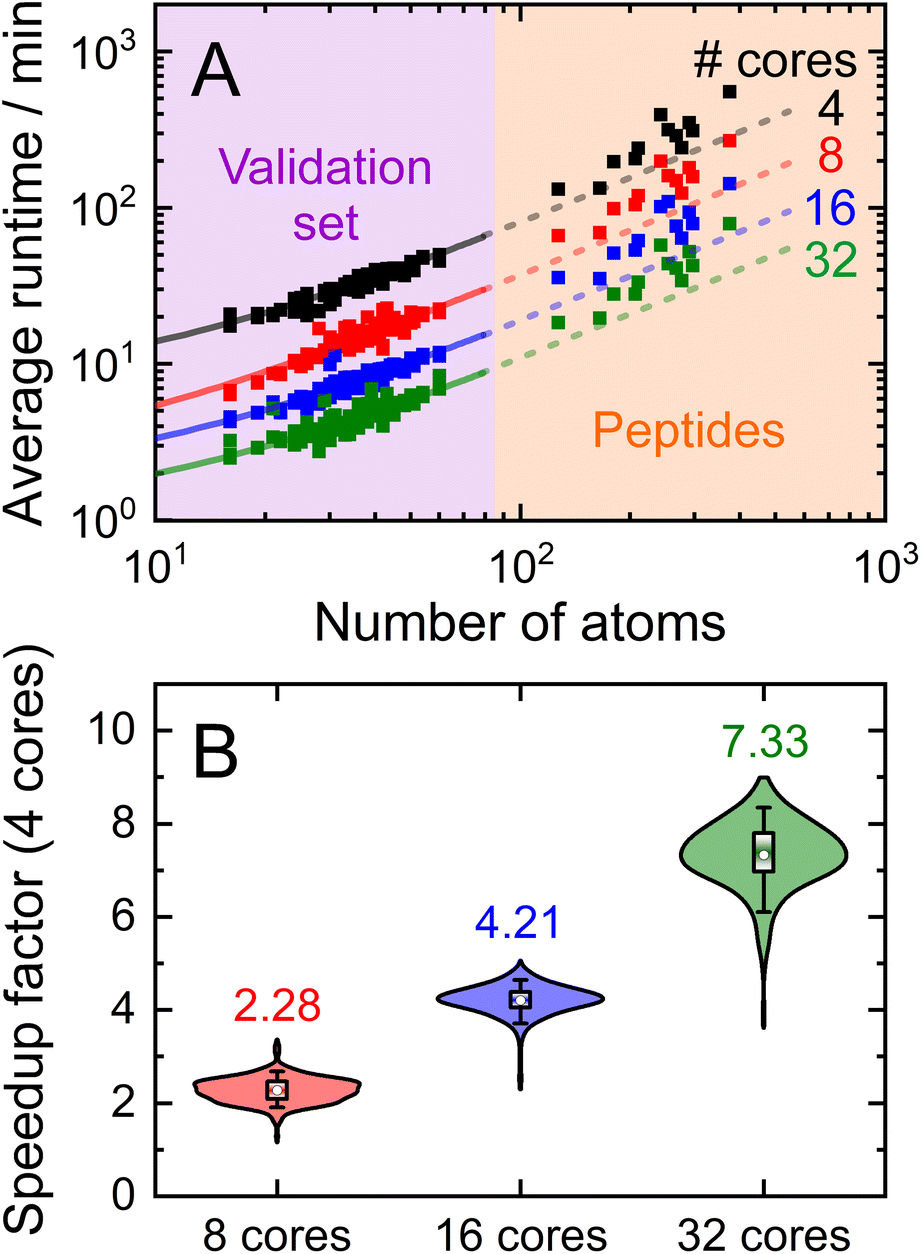 | ||
| Fig. 8 (A) MobCal-MPI 2.0 runtimes for CCS calculations (T = 298 K) of the validation set and 12 peptides as a function of the number of atoms. Calculations used 4 (black), 8 (red), 16 (blue), or 32 (green) cores in parallel. Linear regression is performed on the validation set, the lines for which are extrapolated to the peptides. (B) Violin plot showing the distribution of speedup factors from using 8, 16, or 32 cores compared to 4 cores. All runtimes are reported as the average from three CCS evaluations that employ different seed numbers on the same grid size (itn = 10, inp = 96, and imp = 512). | ||
Linear regression of the averaged runtimes for the validation set with respect to the number of atoms yields slopes that follow an inverse relationship with the number of cores (Fig. S9†). This indicates efficient code parallelization, where doubling the number of cores approximately halves the runtime. This trend can also be observed in Fig. 8B, where the distributions of the individual speedup factors for all conformers in the validation and peptide set are shown as violin plots. The averages of these distributions reflect the aforementioned speed increase, which is to be expected as the total number of collision events sampled is evenly distributed among all cores (i.e., itn × inp × imp). Only for 32 cores do we observe a slightly lower average speedup than the expected value of 8 (as compared to runtime for 4 cores), suggesting the presence of a small parallel execution overhead. Naturally, the absolute runtimes heavily depend on the computing system used, so the runtimes reported here, which were assessed using 2nd generation AMD EPYC processers (AMD Rome 7532 @ 2.40 GHz), will vary from other systems. Nevertheless, calculation of “routine” small molecules (i.e., those containing less than 70 atoms) complete in less than 30 minutes on 8 cores, highlighting the efficiency with which MobCal-MPI 2.0 can compute accurate CCSs to complement experimental results.
Conclusions
This study presents the latest version of the parallelized CCS calculation suite MobCal-MPI 2.0, which significantly improves the handling of collision dynamics with N2. Owing to the diatomic nature of molecular N2, the vdW component of the ion-neutral interaction potential can be evaluated in two ways. In the first approach, N2 can be treated as pseudo-atomic entity, whereby the pairwise interactions that determine the vdW component of the ion-neutral interaction potential are calculated with respect to its centre of mass (CoM). The CoM approach was shown to be erroneous at short ion-neutral distances, where the repulsive portion of the interaction potential is strongly affected by the orientation of N2 relative to the molecule. Consequently, the methodology to evaluate the vdW component was modified to a second approach that considers the averaged, pairwise interaction between each atom in the molecule and each nitrogen atom in the N2 collision partner (Avg-N2). By optimizing the vdW parameters for both the CoM and Avg-N2 methods and evaluating the RMSE between computed and experimental CCSs, it was determined that the Avg-N2 approach slightly outperforms the CoM in terms of calculating CCSs at T = 298 K. Specifically, the Avg-N2 approach exhibits a RMSE of 2.16%, whereas the CoM approach exhibits a RMSE of 2.27% for a diverse set of 50 molecules that were not used to optimize the vdW parameters (i.e., the validation set). This increased accuracy will provide practitioners with greater confidence in assigning experimental mobility data to analyte structures.Because the calculation of CCSs is based on a finite number of collision events, there are inherent statistical uncertainties associated with the computed values. We have made modifications to the workflow to evaluate these uncertainties accurately. In MobCal-MPI 2.0, uncertainties in CCS calculations emerge from the choice of the three sampling parameters, namely: (1) the number of cycles in which collision events are sampled (itn), (2) the number of relative velocities of the ion-neutral pair that are sampled (inp), and (3) the number of impact parameter and ion-neutral orientations (imp). For routine CCS and low-field mobility calculations, we find that settings of itn = 10, inp = 104, and imp = 512 yield an uncertainty of 0.97%. For higher precision, we recommend settings of itn = 10, inp = 200, and imp = 768 or 1024, which reduces the uncertainty in the calculated CCS and low-field mobilities to 0.57%.
To meet the growing demand for high-field mobility computations, the second-order approximation of 2TT was implemented in MobCal-MPI 2.0 alongside an empirical correction. This addition allows for the evaluation of CCS and ion mobility at multiple field strengths that are defined by a range of effective temperatures. When augmented with the empirical correction to 2TT, which corrects for the underestimation of ion mobilities at high field strengths,71 MobCal-MPI 2.0 accurately predicts the high-field mobilities of a set of 132 analytes. Specifically, the high-field mobility data generated by MobCal-MPI 2.0 was used to reproduce the DMS dispersion plots of the 132 analytes, yielding an average error of only −0.4 V in compensation voltage (CV) at the highest separation voltage sampled (4000 V). This deviation translates to a relative error of less than 4% in the capability of MobCal-MPI 2.0 to compute high-field DMS data at 136 Td (with an electrode spacing of 1 mm, T = 373 K, and p = 1 atm).
Another notable change of MobCal-MPI 2.0 compared to its predecessor is the modification of the velocity grid (inp) from a weighted approach (i.e., greater density of points at the maximum of the distribution of velocities at Teff) to a linear grid spacing. Implementing the linear spacing for the inp grid enables the evaluation of collision integrals using a single set of trajectories. In contrast, the non-linear spacing of the weighted inp grid in the previous version of MobCal-MPI required the revaluation of collision integrals for each temperature desired by the user. The introduction of the linear grid in MobCal-MPI 2.0 results in considerably faster CCS computations compared to the previous version; if a user requires CCSs at n effective temperatures, MobCal-MPI 2.0 can accomplish the task n times faster than MobCal-MPI.
Further benchmarking of MobCal-MPI 2.0 reveals its ability to compute low- and high-field mobility data with exceptional efficiency. For example, the CCS of an ion composed of 70 atoms can be obtained in approximately 30 minutes when using 8 cores in parallel. We also find that the decrease in calculation times scales roughly linearly with the number of cores employed; a small parallel execution overhead is observed only when 32 cores are used. We believe that MobCal-MPI 2.0 will be a valuable tool for the IMS community, who can use this code to support their experimental findings with accurate models of analyte mobility/CCS. Although no CCS calculation method is free of systematic biases, the calibration, validation, and high-field validation sets were meticulously selected to encompass a diverse range of functional groups that span the molecular space defined by the MMFF94 forcefield. However, our datasets do not contain anionic or metal adducted species, begging the question of whether the accuracy of MobCal-MPI 2.0 extends to these analytes. As we continue to broaden our collection of low- and high-field mobility data, we plan to evaluate the capability of MobCal-MPI 2.0 to model the mobilities of anionic and metal-adducted species, and to investigate the impact of inelasticity and vibrational broadening on computed mobilities.
Author contributions
A.H. conceptualized, developed, and implemented updates to MobCal-MPI 2.0 (including coding). C.I. created the datasets and conducted the performance/benchmarking calculations. A.H. and C.I. wrote the manuscript. W.S.H. supervised the project. All authors contributed to the final version of the manuscript.Conflicts of interest
There are no conflicts to declare.Acknowledgements
The authors would like to thank Dr Jeff Crouse for his help during the early stages of this work. Further, the authors would like to acknowledge the high-performance computing support from the Digital Research Alliance of Canada. W. S. H. would like to acknowledge the financial support provided by the Natural Sciences and Engineering Research Council (NSERC) of Canada in the form of Discovery and Alliance grants. Further, W. S. H. acknowledges the support from the InnoHK Initiative and the Hong Kong Special Administrative Region Government. A. H. gratefully acknowledges this work being funded by the Deutsche Forschungsgemeinschaft (DFG, German Research Foundation) – 449651261. C. I. acknowledges financial support from the Government of Canada for the Vanier Canada Graduate Scholarship.References
- F. Lanucara, S. W. Holman, C. J. Gray and C. E. Eyers, Nat. Chem., 2014, 6, 281–294 CrossRef CAS PubMed.
- J. C. May and J. A. McLean, Anal. Chem., 2015, 87, 1422–1436 CrossRef CAS PubMed.
- J. N. Dodds and E. S. Baker, J. Am. Soc. Mass Spectrom., 2019, 30, 2185–2195 CrossRef CAS PubMed.
- V. Gabelica, A. A. Shvartsburg, C. Afonso, P. Barran, J. L. P. Benesch, C. Bleiholder, M. T. Bowers, A. Bilbao, M. F. Bush, J. L. Campbell, I. D. G. Campuzano, T. Causon, B. H. Clowers, C. S. Creaser, E. De Pauw, J. Far, F. Fernandez-Lima, J. C. Fjeldsted, K. Giles, M. Groessl, C. J. Hogan, S. Hann, H. I. Kim, R. T. Kurulugama, J. C. May, J. A. McLean, K. Pagel, K. Richardson, M. E. Ridgeway, F. Rosu, F. Sobott, K. Thalassinos, S. J. Valentine and T. Wyttenbach, Mass Spectrom. Rev., 2019, 38, 291–320 CrossRef CAS PubMed.
- E. S. Baker, E. A. Livesay, D. J. Orton, R. J. Moore, W. F. Danielson, D. C. Prior, Y. M. Ibrahim, B. L. LaMarche, A. M. Mayampurath, A. A. Schepmoes, D. F. Hopkins, K. Tang, R. D. Smith and M. E. Belov, J. Proteome Res., 2010, 9, 997–1006 CrossRef CAS PubMed.
- A. L. Rister and E. D. Dodds, J. Chromatogr. B: Anal. Technol. Biomed. Life Sci., 2020, 1137, 121941 CrossRef CAS PubMed.
- E. A. Mason and E. W. McDaniel, Transport Properties of Ions in Gases, Wiley-VCH, New York, NY, USA, 1988 Search PubMed.
- E. A. Mason and H. W. Schamp, Ann. Phys., 1958, 4, 233–270 CAS.
- P. Langevin, Ann. Chim. Phys., 1905, 5, 245–288 CAS.
- V. Gabelica and E. Marklund, Curr. Opin. Chem. Biol., 2018, 42, 51–59 CrossRef CAS PubMed.
- J. C. May, C. B. Morris and J. A. McLean, Anal. Chem., 2017, 89, 1032–1044 CrossRef CAS PubMed.
- I. A. Buryakov, E. V. Krylov, E. G. Nazarov and U. K. Rasulev, Int. J. Mass Spectrom. Ion Processes, 1993, 128, 143–148 CrossRef CAS.
- T.-C. Chen, Y. M. Ibrahim, I. K. Webb, S. V. B. Garimella, X. Zhang, A. M. Hamid, L. Deng, W. E. Karnesky, S. A. Prost, J. A. Sandoval, R. V. Norheim, G. A. Anderson, A. V. Tolmachev, E. S. Baker and R. D. Smith, Anal. Chem., 2016, 88, 1728–1733 CrossRef CAS PubMed.
- C. D. Chouinard, G. Nagy, I. K. Webb, T. Shi, E. S. Baker, S. A. Prost, T. Liu, Y. M. Ibrahim and R. D. Smith, Anal. Chem., 2018, 90, 10889–10896 CrossRef CAS PubMed.
- X. Zheng, N. A. Aly, Y. Zhou, K. T. Dupuis, A. Bilbao, V. L. Paurus, D. J. Orton, R. Wilson, S. H. Payne, R. D. Smith and E. S. Baker, Chem. Sci., 2017, 8, 7724–7736 RSC.
- K. M. Hines, D. H. Ross, K. L. Davidson, M. F. Bush and L. Xu, Anal. Chem., 2017, 89, 9023–9030 CrossRef CAS PubMed.
- A. D. Rolland and J. S. Prell, TrAC, Trends Anal. Chem., 2019, 116, 282–291 CrossRef CAS PubMed.
- B. B. Schneider, E. G. Nazarov, F. Londry, P. Vouros and T. R. Covey, Mass Spectrom. Rev., 2016, 35, 687–737 CrossRef CAS PubMed.
- A. T. Kirk, D. Grube, T. Kobelt, C. Wendt and S. Zimmermann, Anal. Chem., 2018, 90, 5603–5611 CrossRef CAS PubMed.
- A. Haack, J. R. Bissonnette, C. Ieritano and W. S. Hopkins, J. Am. Soc. Mass Spectrom., 2022, 33, 535–547 CrossRef CAS PubMed.
- V. D. Gandhi and C. Larriba-Andaluz, Anal. Chim. Acta, 2021, 1184, 339019 CrossRef CAS PubMed.
- V. D. Gandhi, K. Short, L. Hua, I. Rodríguez and C. Larriba-Andaluz, J. Aerosol Sci., 2023, 169, 106122 CrossRef CAS.
- T. Kihara, Rev. Mod. Phys., 1953, 25, 844–852 CrossRef.
- L. A. Viehland and E. A. Mason, Ann. Phys., 1975, 91, 499–533 CAS.
- L. A. Viehland and E. A. Mason, Ann. Phys., 1978, 110, 287–328 CAS.
- S. L. Lin, L. A. Viehland and E. A. Mason, Chem. Phys., 1979, 37, 411–424 CrossRef CAS.
- L. A. Viehland and S. L. Lin, Chem. Phys., 1979, 43, 135–144 CrossRef CAS.
- L. A. Viehland, Chem. Phys., 1994, 179, 71–92 CrossRef.
- T. A. Halgren, J. Comput. Chem., 1996, 17, 490–519 CrossRef CAS.
- T. A. Halgren, J. Comput. Chem., 1996, 17, 520–552 CrossRef CAS.
- I. Campuzano, M. F. Bush, C. V. Robinson, C. Beaumont, K. Richardson, H. Kim and H. I. Kim, Anal. Chem., 2012, 84, 1026–1033 CrossRef CAS PubMed.
- T. Wu, J. Derrick, M. Nahin, X. Chen and C. Larriba-Andaluz, J. Chem. Phys., 2018, 148, 074102 CrossRef PubMed.
- G. Paglia, J. P. Williams, L. Menikarachchi, J. W. Thompson, R. Tyldesley-Worster, S. Halldórsson, O. Rolfsson, A. Moseley, D. Grant, J. Langridge, B. O. Palsson and G. Astarita, Anal. Chem., 2014, 86, 3985–3993 CrossRef CAS PubMed.
- J. W. Lee, H. H. L. Lee, K. L. Davidson, M. F. Bush and H. I. Kim, Analyst, 2018, 143, 1786–1796 RSC.
- L. Righetti, A. Bergmann, G. Galaverna, O. Rolfsson, G. Paglia and C. Dall'Asta, Anal. Chim. Acta, 2018, 1014, 50–57 CrossRef CAS PubMed.
- J. Regueiro, N. Negreira and M. H. G. Berntssen, Anal. Chem., 2016, 88, 11169–11177 CrossRef CAS PubMed.
- L. Bijlsma, R. Bade, A. Celma, L. Mullin, G. Cleland, S. Stead, F. Hernandez and J. V. Sancho, Anal. Chem., 2017, 89, 6583–6589 CrossRef CAS PubMed.
- A. Bauer, J. Kuballa, S. Rohn, E. Jantzen and J. Luetjohann, J. Sep. Sci., 2018, 41, 2178–2187 CrossRef CAS PubMed.
- C. Ieritano, J. Crouse, J. L. Campbell and W. S. Hopkins, Analyst, 2019, 144, 1660–1670 RSC.
- C. Ieritano, A. Lee, J. Crouse, Z. Bowman, N. Mashmoushi, P. M. Crossley, B. P. Friebe, J. L. Campbell and W. S. Hopkins, Anal. Chem., 2021, 93, 8937–8944 CrossRef CAS PubMed.
- C. Ieritano, J. L. Campbell and W. S. Hopkins, Analyst, 2021, 146, 4737–4743 RSC.
- J. Yang and Y. Zhang, Nucleic Acids Res., 2015, 43, W174–W181 CrossRef CAS PubMed.
- W. Zheng, C. Zhang, Y. Li, R. Pearce, E. W. Bell and Y. Zhang, Cells Rep. Methods, 2021, 1, 100014 CrossRef CAS PubMed.
- J.-D. Chai and M. Head-Gordon, J. Chem. Phys., 2008, 128, 084106 CrossRef PubMed.
- Y.-S. Lin, G.-D. Li, S.-P. Mao and J.-D. Chai, J. Chem. Theory Comput., 2013, 9, 263–272 CrossRef CAS PubMed.
- S. Grimme, J. Antony, S. Ehrlich and H. Krieg, J. Chem. Phys., 2010, 132, 154104 CrossRef PubMed.
- F. Weigend and R. Ahlrichs, Phys. Chem. Chem. Phys., 2005, 7, 3297–3305 RSC.
- F. Weigend, Phys. Chem. Chem. Phys., 2006, 8, 1057–1065 RSC.
- C. M. Breneman and K. B. Wiberg, J. Comput. Chem., 1990, 11, 361–373 CrossRef CAS.
- J. Tao, J. P. Perdew, V. N. Staroverov and G. E. Scuseria, Phys. Rev. Lett., 2003, 91, 146401 CrossRef PubMed.
- F. Neese, Wiley Interdiscip. Rev.: Comput. Mol. Sci., 2012, 2, 73–78 CAS.
- F. Neese, F. Wennmohs, U. Becker and C. Riplinger, J. Chem. Phys., 2020, 152, 224108 CrossRef CAS PubMed.
- M. Álvarez-Moreno, C. de Graaf, N. López, F. Maseras, J. M. Poblet and C. Bo, J. Chem. Inf. Model., 2015, 55, 95–103 CrossRef PubMed.
- C. Bo, F. Maseras and N. López, Nat. Catal., 2018, 1, 809–810 CrossRef.
- N. M. O'Boyle, M. Banck, C. A. James, C. Morley, T. Vandermeersch and G. R. Hutchison, J. Cheminf., 2011, 3, 33 Search PubMed.
- C. Ieritano and W. S. Hopkins, Mater. Today Commun., 2021, 27, 102226 CrossRef CAS.
- L. Boltzmann, Sitzungsber. Akad. Wiss. Wien, 1872, 66, 275–370 Search PubMed.
- S. Chapman and T. G. Cowling, The Mathematical Theory of Non-Uniform Gases, Cambridge University Press, London, UK, 3rd edn, 1970 Search PubMed.
- J. O. Hirschfelder, C. F. Curtiss and R. B. Bird, Molecular Theory of Gases and Liquids, John Wiley & Sons, Inc., New York, NY, USA, Corrected, 1964 Search PubMed.
- J. Aisbett, J. M. Blatt and A. H. Opie, J. Stat. Phys., 1974, 11, 441–456 CrossRef.
- A. A. Shvartsburg and M. F. Jarrold, Chem. Phys. Lett., 1996, 261, 86–91 CrossRef CAS.
- M. F. Mesleh, J. M. Hunter, A. A. Shvartsburg, G. C. Schatz and M. F. Jarrold, J. Phys. Chem., 1996, 100, 16082–16086 CrossRef CAS.
- J. H. Lii and N. L. Allinger, J. Am. Chem. Soc., 1989, 111, 8576–8582 CrossRef CAS.
- H. Kim, H. I. Kim, P. V. Johnson, L. W. Beegle, J. L. Beauchamp, W. A. Goddard and I. Kanik, Anal. Chem., 2008, 80, 1928–1936 CrossRef CAS PubMed.
- H. I. Kim, H. Kim, E. S. Pang, E. K. Ryu, L. W. Beegle, J. A. Loo, W. A. Goddard and I. Kanik, Anal. Chem., 2009, 81, 8289–8297 CrossRef CAS PubMed.
- C. Graham, D. A. Imrie and R. E. Raab, Mol. Phys., 1998, 93, 49–56 CrossRef CAS.
- C. Ieritano and W. S. Hopkins, Phys. Chem. Chem. Phys., 2022, 19–24 Search PubMed.
- H.-S. Hahn and E. A. Mason, Chem. Phys. Lett., 1971, 9, 633–635 CrossRef CAS.
- W. S. Hopkins, in Advances in Ion Mobility-Mass Spectrometry: Fundamentals, Instrumentation and Applications, ed. W. A. Donald and J. S. Prell, Elsevier B.V., 2019, vol. 83, pp. 83–122 Search PubMed.
- A. Haack, J. Crouse, F.-J. Schlüter, T. Benter and W. S. Hopkins, J. Am. Soc. Mass Spectrom., 2019, 30, 2711–2725 CrossRef CAS PubMed.
- W. F. Siems, L. A. Viehland and H. H. Hill, Analyst, 2016, 141, 6396–6407 RSC.
- E. Krylov, E. G. Nazarov, R. A. Miller, B. Tadjikov and G. A. Eiceman, J. Phys. Chem. A, 2002, 106, 5437–5444 CrossRef CAS PubMed.
- A. Haack and W. S. Hopkins, J. Am. Soc. Mass Spectrom., 2022, 33, 2250–2262 CrossRef CAS PubMed.
- C. Larriba-Andaluz and J. S. Prell, Int. Rev. Phys. Chem., 2020, 39, 569–623 Search PubMed.
- L. A. Viehland, S. L. Lin and E. A. Mason, Chem. Phys., 1981, 54, 341–364 CrossRef CAS.
- A. A. Shvartsburg, S. V. Mashkevich and K. W. M. Siu, J. Phys. Chem. A, 2000, 104, 9448–9453 CrossRef CAS.
- A. A. Shvartsburg, T. Bryskiewicz, R. W. Purves, K. Tang, R. Guevremont and R. D. Smith, J. Phys. Chem. B, 2006, 110, 21966–21980 CrossRef CAS PubMed.
- C. Schaefer, A. T. Kirk, M. Allers and S. Zimmermann, J. Am. Soc. Mass Spectrom., 2020, 31, 2093–2101 CrossRef CAS PubMed.
- V. D. Gandhi, J. Lee, L. Hua, M. Latif, C. J. Hogan and C. Larriba-Andaluz, Anal. Chem., 2023, 95, 7941–7949 CrossRef CAS PubMed.
- D. Morsa, V. Gabelica and E. De Pauw, Anal. Chem., 2011, 83, 5775–5782 CrossRef CAS PubMed.
- D. Morsa, E. Hanozin, G. Eppe, L. Quinton, V. Gabelica and E. De Pauw, Anal. Chem., 2020, 92, 4573–4582 CrossRef CAS PubMed.
- S. Poyer, C. Comby-Zerbino, C. M. Choi, L. MacAleese, C. Deo, N. Bogliotti, J. Xie, J.-Y. Salpin, P. Dugourd and F. Chirot, Anal. Chem., 2017, 89, 4230–4237 CrossRef CAS PubMed.
Footnotes |
| † Electronic supplementary information (ESI) available: Further information on the reported updates to MobCal-MPI (PDF); listing of all compounds in the calibration, validation, and high-field validation set (XLSX); XYZ structures and partial charges of all compounds (ioChem-bd database, https://iochem-bd.bsc.es/browse/handle/100/285126). See DOI: https://doi.org/10.1039/d3an00545c |
| ‡ These authors contributed roughly equally to this work. |
| This journal is © The Royal Society of Chemistry 2023 |