Artefact removal from micrographs with deep learning based inpainting

Abstract

Imaging is critical to the characterisation of materials. However, even with careful sample preparation and microscope calibration, imaging techniques can contain defects and unwanted artefacts. This is particularly problematic for applications where the micrograph is to be used for simulation or feature analysis, as artefacts are likely to lead to inaccurate results. Microstructural inpainting is a method to alleviate this problem by replacing artefacts with synthetic microstructure with matching boundaries. In this paper we introduce two methods that use generative adversarial networks to generate contiguous inpainted regions of arbitrary shape and size by learning the microstructural distribution from the unoccluded data. We find that one benefits from high speed and simplicity, whilst the other gives smoother boundaries at the inpainting border. We also describe an open-access graphical user interface that allows users to utilise these machine learning methods in a ‘no-code’ environment.

---

1 Introduction

Characterising materials with imaging techniques is critical to understanding their structure–function relationship. Microstructural images, alongside statistical image analysis and physical simulations, allow for microstructural features to be linked to material behaviour.^1–3 This in turn facilitates material design and optimisation. Unfortunately, samples can suffer from defects during preparation and artefacts can be caused by disturbances during imaging, resulting in regions of the image being unusable for analysis and simulation (hereafter referred to as occluded regions). Some common sources of occlusions are surface scratches during sample cutting,⁴ charging effects in scanning electron microscopy (SEM),⁵ and regions of an image being corrupted by software errors. Whilst the imaging would ideally be repeated in the hope of obtaining a clean micrograph (if the imaging technique is not destructive), this is a time consuming process, and particularly challenging if large, representative images are needed. Alternatively, it is possible to replace these occluded regions with reconstructed microstructure post hoc, thus reducing the cost of characterisation. This process is called inpainting.

Broadly, there are two approaches to inpainting – classical statistical reconstruction⁶ and machine learning reconstruction. A variety of classical reconstruction techniques exist, such as diffusion-based^7–9 and structure/exemplar-based.^10–12 The most ubiquitous technique is exemplar-based inpainting, whereby the occluded region is filled in from the outer edge to center with the best matching patches that are ‘copied-and-pasted’ from the unoccluded region.^13–16 Barnes et al. proposed the PatchMatch algorithm for fast patch search using the natural coherency of the image.¹² Tran et al. extended the PatchMatch algorithm to microstructural inpainting.^17,18 They outline that typically, machine learning based inpainting requires large, labelled datasets, and that their classical statistical reconstruction method does not. This approach can be used to reconstruct grayscale image data, however, with patch-based approaches, the reconstructed region will contain exactly copied regions which may be unrealistic.¹⁹

Convolutional neural networks (CNNs) form the basis of many visual machine learning tasks. The majority of generative methods that use CNNs take the form of autoencoders,²⁰ diffusion models²¹ or generative adversarial networks (GANs).²² General purpose inpainting models using these methods have been developed, which have been extremely successful across many applications.^23–27 However, many of the state-of-the-art (SOTA) models require large labelled datasets for training from scratch or fine-tuning pretrained models.^28,29 SOTA models are also often very deep (i.e. many hidden layers in the CNN) to allow the synthesis of a wide variety of complex features, which makes training computationally expensive and, therefore, only available to those with access to high performance computers, resulting in poor accessibility to the general community. It is not only the accessibility of training that is limited, but also the application of trained models is often restricted. It is possible to apply these existing large scale image models to material science problems and depending on the application the success is varied. What is not possible, is the direct integration of materials science assumptions and requirements, such as statistical homogeneity. As such, an opportunity exists for an open-source inpainting method specifically designed for materials science that is computationally inexpensive to train and also works well in scenarios where data is severely limited.

Microstructural image data has properties that can be exploited in order to address the issues outlined above. Often micrographs are taken of the bulk of a material, and the resulting data is homogeneous. Therefore, any large enough patch of microstructure is statistically equivalent to any other patch. This allows a single image to be batched into a statistically equivalent set of smaller images, hence forming a training dataset for a generation algorithm. This eases the requirement on collecting a large dataset consisting of many distinct images, which would be the case if each entire image was a single instance of a training example. Furthermore, once a generative model has been trained on a statistically representative dataset, it can then be used to generate arbitrarily large images that would be impractical to collect experimentally. This idea was demonstrated by Gayon-Lombardo et al., who developed a GAN framework with an adjustable input size.³⁰ Unlike the majority of GAN models, where the output size of the generator must match that of the entire generated image, the output microstructural generators need only be big enough to capture key features and can therefore be far smaller. The relative simplicity of microstructural features also reduces the required number of parameters, shrinking training times and reducing memory requirements. These properties of microstructural data greatly reduce the memory and compute requirements when training generation algorithms, and also mitigate the need for large training datasets. However, it also means the method is restricted to cases where the data is homogeneous (i.e. samples taken from any random point in the image are statistically equivalent).

GANs are a family of machine learning models characterised by the use of two networks competing in an adversarial game. They are capable of generating samples from an underlying probability distribution of an input training dataset. Mosser et al. introduced GANs as a method for reconstructing synthetic realisations of a homogeneous microstructure.³¹ Further methods have been developed to reconstruct 3D multi-phase microstructure, generate 3D images from 2D data, and fuse multi-modal datasets together.^30,32,33 These models make use of some assumptions about microstructural image data outlined earlier to shrink the memory and compute requirements of training. These methods have successfully demonstrated the ability to generate synthetic volumes that are statistically indistinguishable from the training data, but do not solve the specific problem of inpainting. GANs have emerged as the most common machine learning method for inpainting microstructure. Ma et al. developed an automatic inpainting algorithm which involves two steps, firstly the classification and segmentation of the occluded region, followed by inpainting.³⁴ A U-Net performs the segmentation of the damaged region, and an EdgeConnect model performs the inpainting.^35,36 This method requires a large dataset of manually labelled damaged regions, which makes this method hard to generalise to all types of defect. Karamov et al. developed a GAN-based method, with an autoencoder generator for inpainting grayscale, 3D, anisotropic micro-CT images.³⁷ This method demonstrated moderate success but struggled to form contiguous boundaries. The resulting inpainted microstructure had an observable hard border of non-matching pixels. Although having discontiguous borders does not affect some global statistics such as volume fraction or pixel value distributions, it is extremely important for microstructural scale modelling. Consider a diffusion simulation on a porous medium to extract the tortuosity factor,³⁸ any discontiguities in the phase boundaries may have a significant impact on the resulting flow field.

This paper outlines two novel GAN-based methods for inpainting microstructural image data without the need for large datasets or labelled data. These methods are designed to be applied in different scenarios. Each approach seeks to satisfy two key requirements for successful inpainting, namely the generation of realistic features to replace the occluded region, and the matching of these features to existing microstructure at the inpainting boundary. The first method, generator optimisation (G-opt), uses a combination of a standard GAN loss (maximise realness of generated data according to the discriminator) and a content loss (minimise the pixel-wise difference between generated and ground truth boundary) to simultaneously address both goals. The resulting generator is well optimised for a specific inpaint region, but cannot be applied to other defect regions without retraining. The second method, seed optimisation (Z-opt), decouples the two requirements by first training a GAN to generate realistic microstructure, and then searching the latent space for a good boundary match. This means the generator can be applied to any occluded region in the image after training, but boundary matching can be less successful. It is important to note that these methods are stochastic, and that the inpainted region is not meant to reconstruct the ground truth. Instead these techniques aim to synthesise entirely new, but statistically equivalent regions of microstructure, whilst maintaining a contiguous border with the unoccluded region. These generated inpaintings do not represent the ‘true’ underlying microstructure, but rather one of many statistically indistinguishable synthetic possibilities. Due to the stochastic nature of these methods, there is no single solution to this problem, and a family of solutions can be synthesised.

Additionally, in Section 5 this paper presents a graphical user interface (GUI) through which users can easily apply these methods to their own data. The purpose of this is to provide democratic access to a tool for materials scientists from a range of disciplines. The GUI requires no coding experience and has been made open source to accompany this paper.

2 Methods

The exact architecture for the generator (G) and discriminator (D) can be tweaked for different use cases. To fairly compare the methods, it was decided that the same network architectures and hyperparameters should be used for both. These are shown in the ESI Table 2.† In this study, we explore inpainting of n-phase, colour and grayscale images. For n-phase segmented images, the final activation layer of the generator is an n-channel softmax, where the output value in each channel can be interpreted as the ‘confidence’ that the given pixel belongs to the phase. In post-processing, the maximum confidence phase is selected and the output is shown as segmented into three phases. Otherwise, the final layer of the output is a sigmoid. In the results presented in this paper, both methods are also trained for the same number of iterations and for each method no cherry picking of results was performed. To demonstrate this, the ESI† contains a multitude of generated examples (ESI Fig. 3–5†).

2.1 Generator optimisation

As previously described, the G-opt technique involves training a generator model that can synthesise realistic inpainted regions. It incorporates a content loss between the generated and real boundary to enforce feature continuity, and a conventional Wasserstein loss to ensure realistic features.^39,40Table 1 describes the training regime for G. When computing the content loss, a fixed seed is used as the input, then the mean squared error (MSE) is calculated on a frame (a 16 pixel wide band around the outside of the region) of the real and fake data. The fixed seed is kept the same throughout training when calculating the content loss, and saved alongside the model weights after training, as it is this specific seed which G learns to map to the matching boundaries. It is important to note that during training, the Wasserstein loss must be calculated without the fixed seed region, and is instead trained with a random seed, as otherwise the constant frame that it generates could be used by the discriminator to identify fake samples.

Table 1 Generator optimisation algorithm

Require G, the generator function; D, the discriminator function; c, the coefficient of the content loss multiplication (default 1); gt, the ground truth region selected for inpainting; CL, the content loss function (mean squared error); FR, frame function that takes only the pixels in the 16 pixel boundary around the occluded region; S, seed function that takes the fixed seed and replaces possible central elements with random values; gp, gradient penalty; imax, maximum number of iterations; , standard normal distribution; All batch operations and optimization parameters are not shown for simplicity, we refer the reader to the codes at the project's repository for specific parameter details, including details about the implementation of the gradient penalty
⊳% training%
1	Select inpaint region of size d × d
2
3	For i = 0, …, imax do
4
5	Fake ← G(zrand)
6	Real ← sample a batch of training images from the unoccluded region
7	l D ← D(fake) − D(real) + gp
8	Backpropagate and update the weights of D from the loss lD
9	If 10∣i then
10
11	Fake ← G(zrand)
12	Fixed ← G(zfixed) output has dimensions (d + 16) × (d + 16)
13	l CL ← CL(FR(gt), FR(fixed)) take content loss between the 16 pixel frame of gt and fixed
14	l G ← −D(fake) + c × lCL
15	Back propagate and update the weights of G from the loss lG
⊳% evaluation%
16	z eval ← S(zfixed)
17	Out ← G(zeval)
18	Inpaint ← out, gt replace d × d occluded region with output of G (with frame removed)

---

Interestingly, the architecture of G remains the same for all sizes of occluded region. To match the network output size to the occluded region, we change the spatial size of the random input seed, which is an established technique for controlling image dimensions when generating homogeneous textures of material micrographs. In the standard network that we use, increasing the input seed size by 1 results in an output size increase of 8. The size of the selected occluded region is thus restricted to be a multiple of 8 pixels in each dimension, allowing for an associated integer seed size. This calculated seed size is increased by four (padding of two in each direction) when passed to G in order to generate the boundary region on which the content loss is calculated.

During evaluation, the fixed seed is passed to G and the boundary region of the output is replaced with the boundary region of the original image, such that only the occluded region is replaced. As the seed is fixed, this will generate the exact same inpainting each time G is evaluated. For occluded regions larger than 64 × 64 pixels, the fixed seed can be adjusted by replacing central elements of the seed with random noise. This creates stochastically varying microstructure in the centre of the generated region, but does not alter the generated output at the boundaries.

The methods developed in this paper take a frame of width 16 pixels when calculating the content loss. Transpose convolutions propagate information outwards with each layer, meaning a single seed will affect a whole region of space in the output. In order to safely change the seeds to not affect the border matching, we ensure a buffer of 8 pixels on each side, and a minimum area of 32 pixels in the center to change. Therefore, the minimum seeds size is 10 × 10, as this generates a 64 × 64 pixel image. Above this, the seeds that can be changed scale with the following formula (assuming square seeds): n_Δ = 2 × (n_seed − 10), where n_Δ is the number of central seeds that can be changed if n_seed is the total seed size. For example, for a 12 × 12 seed, a 4 × 4 region can be changed. It is the hyperparameters of the network, specifically the transpose convolutions in the generator, that constrain the minimum size of the inpainting region to 64 × 64 pixels, this is not a fundamental limit and can be altered by adjusting the hyperparameters. For further details and a visual demonstration, the reader is referred to ESI Fig. 2.†

2.2 Seed optimisation

The Z-opt approach separates the tasks of generating realistic microstructure and generating well matched contiguous boundaries. The generator is trained with the usual Wasserstein loss metric and the seed is optimised for inpainting after training. The decoupling of the two optimisation tasks enables the generator to inpaint any region of the micrograph after it has been trained.

The Z-opt is performed by first calculating the MSE between the frame of the generated region and the ground truth. Then, whilst holding the weights of G constant, the MSE is backpropagated to the seed, which is treated as a learnable parameter. If the iterative updates to the seed are unconstrained, its distribution of values deviate significantly from the random normal noise distribution used during training. This is problematic, as although the resulting MSE on the boundary is potentially very low, the central features in the occluded region become unrealistic.

Initially, we attempt to address this deviation through a simple re-normalisation procedure of the seed after each seed update, which can be implemented by subtracting the mean of the seed and dividing by the standard deviation. However, the output of the optimisation after many iterations appeared to deviate from realistic microstructure and become blurry. A histogram of the values of the seed showed that the seed became non-normally distributed, and although retained a mean of 0 and standard deviation of 1, it in fact became bimodal, with two peaks centered around 1 and −1. To keep the seed normally distributed, a KL loss (a statistical measure of distance between two distributions) between the seed and a random normal seed was introduced which anchored the optimised seed to the distribution of random normal seeds. This stopped the more unrealistic features being generated and enforced a normal distribution throughout the optimisation process.

2.3 Inpaint quality analysis

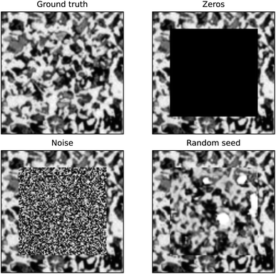
There are two important aspects to validating the ‘goodness’ of the inpainting. Firstly, the inpainted microstructure must retain the statistics of the training data. Secondly, the border between the generated microstructure and original data must be well matched. To validate the first of these, the distribution of volume fractions (VFs) of generated microstructure was calculated. To analyse the contiguity of the border, a technique was developed that compares the distribution of mean squared errors between neighbouring pixels on the boundary.

First, we calculate the difference between the pixels outside the edge of the inpainted region (which belong to the original image) and the pixels inside the edge of the inpainted region (which belong to the generated image). The squares of these differences form a distribution that describes the mean squared error of neighbouring pixels. A ground truth distribution is then calculated by taking the mean squared error between all neighbouring pixels in the original image. A Kolmogorov–Smirnov test for goodness of fit⁴¹ is then used to return the probability that the distribution calculated from the inpainted border and the distribution calculated from the ground truth are the same. For comparison, this border contiguity test was also performed on an inpainting of zeros, uniform noise and the output of a trained generator given an unoptimised random input seed (and therefore agnostic to the border) as shown in Fig. 1.

Fig. 1 The four inpainting examples used to test the border contiguity analysis. The p-values for each test: ground truth = 0.017, zeros = 1.7 × 10⁻¹⁸⁴, noise = 8.2 × 10⁻⁸³, random seed = 6.1 × 10⁻⁴⁶.

The p-value for the ground truth gives a reference value for what ‘perfect’ inpainting looks like for this microstructure, and the order of magnitude of the p-value can be used to compare different inpainting methods, and quantify how discontiguous the border of the inpainting is relative to the ground truth. The ground truth p-value is not necessarily 1, as the KS test is performed between the MSE distributions of neighbouring pixels across the whole image and the border of the ‘to be’ inpainted region. We expect the p-value to be closer to one the more the border region is representative of the global distribution.

3 Results

3.1 N-phase

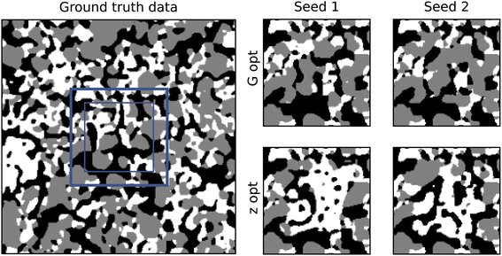
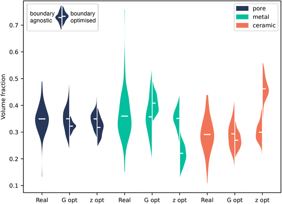
Initially, both methods were tested on a three-phase solid oxide fuel cell anode dataset.⁴² The material was imaged using FIB-SEM and then segmented into three phases: pore (black), metal (grey) and ceramic (white). An occluded region was chosen that did not contain any defects for the purpose of comparison between the ground truth and the generated output. The full images for all training data are shown in ESI Fig. 1.† The results of the inpainting with both methods is shown in Fig. 2.

Fig. 2 The inpainting result for the two methods on a three-phase dataset. The four images on the right contain the ground truth frame (bold blue box) and the inpainted region (thin blue box). The p-values for the contiguity analysis: GT = 1, G-opt = 1, Z-opt = 1, zeros = 2.2 × 10⁻⁵⁹, noise = 3.1 × 10⁻¹²⁰, random seed = 6 × 10⁻¹⁹².

Fig. 3 shows the results of volume fraction analysis on the inpainted microstructures. By enforcing the boundary of our generated volume to match, we naturally restrict the space of possible structures, and therefore we do not necessarily expect to recover exactly the same VF distribution as the ground truth data. However, we do expect our generator to be capable of producing this distribution when given a random boundary agnostic seed. Therefore, in Fig. 3, for each method, two distributions are shown: firstly, where no boundary matching has taken place, and secondly where it has.

Fig. 3 Volume fraction distributions for the three phases of case 1 – SOFC anode. For each phase, the distribution of volume fractions for the ground truth data (real) is shown. The G-opt is split into half violins for a boundary agnostic, i.e. random input seed (left) and for the boundary optimised, i.e. hybrid fixed-random input seed (right). The Z-opt is split into half violins for a boundary agnostic, i.e. random input seed (left) and a boundary optimised, i.e. optimised input seed (right). The distributions are shown across 128 different seeds, but all on the same inpainted region. The mean of the distribution is shown as a white bar.

We first consider the case with no boundary matching. KS tests were performed on each method to compare the distributions of volume fractions to the ground truth, the full results are shown in ESI Table 1.† The p-value is a measure of how probable it is these samples were taken from the same distribution. In the boundary agnostic case, the G-opt method produces distributions with large p-values (0.73–0.97), indicating a good agreement with the ground truth distribution. The boundary agnostic Z-opt method produces smaller p-values (0.022–0.43), revealing poorer agreement with the ground truth. As these generators are identical in architecture and were trained for the same number of iterations, this indicates that the addition of the content loss during training improves the overall quality of the generator.

It is possible that because the content loss is introduced from the start of training, G can immediately start to learn kernels that produce realistic features, without requiring useful information from D. This inevitably speeds up the convergence of G, and also aids in training D, as ‘realness’ of the output of G will be improved earlier in training. Without this content loss, G is entirely reliant on the information from D, and therefore cannot start to learn realistic features until D has learned to discriminate them. It is possible that the benefit G-opt gains from content loss in the early stages of training may be balanced out over longer training times, and that Z-opt may reach the same overall performance, but in more iterations. However, it is important to note that the difference in loss functions means the loss landscapes each method is exploring are fundamentally different, and therefore they will never converge to the exact same solution.

Fig. 3 shows that the boundary optimised VF distributions of the G-opt method are constrained within the bounds of the distribution produced by the boundary agnostic case. This suggests that, although the VF distribution of the boundary matched seed is not similar to the ground truth distribution, the VFs of the generated microstructure are at least a subset of the underlying VF distribution. On the other hand, the boundary optimised Z-opt distribution is significantly offset from the distribution produced by the boundary agnostic case. Specifically, the metal phase shows a significant decrease in volume fraction and the ceramic phase a significant increase in volume fraction. This is also clearly visible in 2, as there appears to be an over representation of the white phase. This can be explained by the seed optimisation process. During training, G is given seeds that are sampled from a random normal distribution. When the seed is optimised post-training, the optimisation pushes the seed into a region where the boundary is best matched, and although the seed is encouraged to retain its normality, this region of latent space may not have been well sampled in training, therefore generating samples that do not follow the same statistics as the underlying data.

To quantify the contiguity of the border, the analysis outlined in Section 2.3 was performed on the inpainted result of both methods. This analysis reveals the G-opt method produces borders that are indistinguishable from the ground truth, yielding a p-value of 1. The Z-opt method performs worse, and produces a more significant result, despite the border not being noticeably discontiguous.

3.2 Grayscale and colour

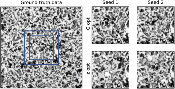
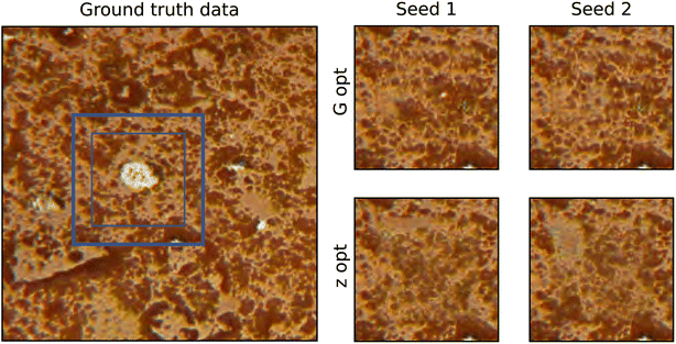
The second case presented in this study is a grayscale image of a hypoeutectoid steel (micrograph 237) taken from DoITPoMS.⁴³ Obtaining a realistic and contiguous output is more difficult for continuous pixel values, and therefore the networks were trained for more iterations.

Fig. 4 shows a comparison of the two methods for the grayscale case. The contiguity analysis reveals a more noticeable disparity between the p-values of the two methods, with G-opt (1.4 × 10⁻⁶) outperforming Z-opt (2.7 × 10⁻¹⁴) by many orders of magnitude. However, the significance value for G-opt is still significantly lower than the ground truth (0.017). This is corroborated by inspecting the inpainting visually as small discontiguities in the G-opt method are visible. The Z-opt method shows much clearer and more distinct boundaries, with some unrealistic features emerging in the bulk.

Fig. 4 The inpainting result for the two methods on a grayscale dataset. The four images on the right contain the ground truth frame (bold blue box) and the inpainted region (thin blue box). The p-values for the contiguity analysis: GT = 0.017, G-opt = 1.4 × 10⁻⁶, Z-opt = 2.7 × 10⁻¹⁴, zeros = 1.7 × 10⁻¹⁸⁴, noise = 8.2 × 10⁻⁸³, random seed = 6.1 × 10⁻⁴⁶.

Analysis of volume fraction of phases is not possible for unsegmented data, which makes assessing the quality of the generated output challenging. Instead of comparing derived microstructural metrics, we plot the distribution of continuous pixel values and compare to the ground truth.

As evident in Fig. 5, the optimisation of the seed drives the generator to output more pixels with the value 1. This was reflected in Fig. 4, as there appeared to be an over representation of white regions in the microstructure. However, the unoptimised Z-opt output appears to contain more 1 s than the ground truth too. This indicates the training has not reached convergence, as the statistical properties of the ground truth have not been recreated. Similarly to the n-phase case, it appears that the content loss in G-opt offers a real advantage to the training and pushes the statistics towards the ground truth.

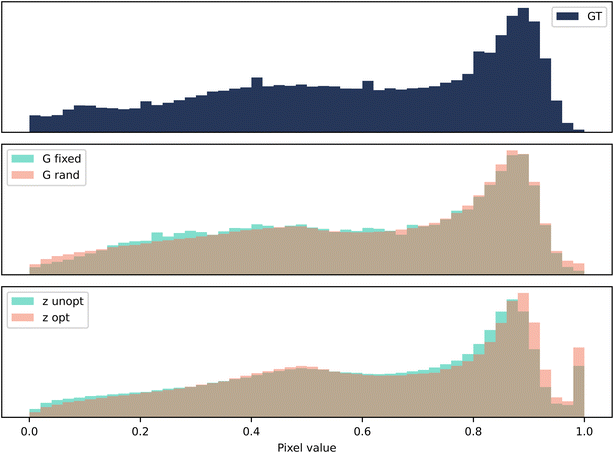Fig. 5 Case 2: grayscale. A histogram of pixel values for 128 samples of size 80 × 80 pixels. The vertical axis is the frequency of occurrence of a particular bin of pixel values.

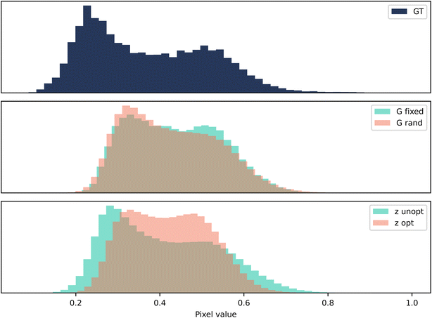
The third case is a colour image of a terracotta pot (micrograph 177) taken from DoITPoMS.⁴³ As colour is an additional level of complexity, the model was trained for 300k iterations. A comparison of the two methods is shown in Fig. 6. For this case, the occluded region contains a material artefact. Contiguity analysis reveals a stark difference in the performance of the two methods, also corroborated by visual inspection. The p values of the G-opt method (1.1 × 10⁻¹³) are many orders of magnitude larger than the Z-opt method (3.7 × 10⁻⁴⁶), and visually the borders appears much more contiguous.

Fig. 6 The inpainting result for the two methods on a colour dataset. The four images on the right contain the ground truth frame (bold blue box) and the inpainted region (thin blue box). The p-values for the contiguity analysis: GT = 4.7 × 10⁻⁵, G-opt = 1.1 × 10⁻¹³, Z-opt = 3.7 × 10⁻⁴⁶, zeros = 0, noise = 0, random seed = 6.5 × 10⁻¹⁷⁰.

The pixel distributions shown in Fig. 7 reveal that both methods fail to replicate the distribution very well. There is a notable change in the shape of the distribution when fixing the seed in G-opt, this appears to flatten the peak of the distribution. This is also observed post-optimisation of the seed in Z-opt, and it seems that this moves it further away from the ground truth. Therefore in both cases, it appears that the fixing of the seed or the seed optimisation reduces the similarity between the ground truth statistics and the statistics of the generated data.

Fig. 7 Case 3: colour. A histogram of pixel values for 128 samples of size 80 × 80 pixels after being transformed to grayscale. The following transformation was used: v_gray = v_colour × [0.2989,0.5870,0.1140]^T. The vertical axis is the frequency of occurrence of a particular bin of pixel values.

4 Discussion

Both methods perform better for n-phase (i.e. segmented images) than for grayscale or colour. The design of our networks makes matching n-phase boundaries easier than grayscale or colour, as for n-phase problems the final activation layer is a softmax. For each pixel, the phase with the highest probability from the softmax is selected, and therefore exact matching of boundary pixels is possible. With grayscale and colour, the output of the generator is continuous, and therefore discontiguous boundary matching is more likely. A marked difference in the accuracy of the two methods arises in the application to grayscale and colour images. In these cases, the G-opt method outperforms the Z-opt method. Intuitively, we can understand this disparity by considering the conditioning of the latent space during training. When the output space becomes continuous rather than discrete, the space of possible microstructures is larger. Therefore, it becomes even less likely that the seed that corresponds to a well matched boundary will exist in a well-conditioned region of the latent space without constraining the space. The G-opt method introduces this constraint, and ensures the seed exists in the latent space.

Variation in the inpainted region when changing the random seed implies over-fitting has not occurred during training.⁴⁴ This demonstrates that the proposed methods do not require large datasets for training. They do, however, rely on the assumption that the data is homogeneous. Additionally, it is important to note that the generated data will only be as statistically representative of the material as the unoccluded region.

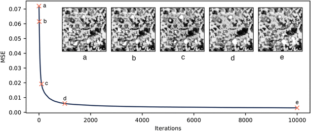
The optimisation of the seed to minimise the content loss appears to push the generator to generate unrealistic microstructure. This was confirmed by the distribution of VFs in Fig. 3. Fig. 8 shows the inpainted micrograph during seed optimisation. This demonstrates that as the seed is optimised the boundary becomes better matched, but some unrealistic features emerge. It is interesting to note that the intermediate results after 100 and 1000 iterations are particularly unrealistic, and that the microstructure returns to more realistic at long optimisation times. This could be because the seed first seeks to satisfy the easier MSE condition on the border, and then searches for a more normal seed distribution to satisfy the KL loss. It is clear that the seed that corresponds to a perfect matching boundary either does not lie in the space of realistic microstructures or at least this process is unable to satisfy both conditions, hence motivating the alternate method.

Fig. 8 The output of G and the MSE throughout the seed optimisation process.

As previously mentioned, both methods were trained using the same hyperparameters (ESI Table 2), with the only difference in the training procedure being the fixing of the seed and the inclusion of the content loss. The G-opt method therefore takes longer per iteration. However, once trained the G-opt method is much faster to evaluate, with the Z-opt requiring a new optimisation for each new instance. Overall, there is a trade-off between training time, generation time and quality, meaning a method should be chosen according to the application.

Ultimately, the user determines whether or not the model or optimisation has converged. The hyperparameters in this paper are a guide, but can be tuned for different use cases. For example, for more complex materials, the number of filter layers in the networks can be increased, the training time extended and the number of optimisation iterations increased. The volume fraction and border contiguity analysis outlined in this paper are useful guides when comparing different methods and sets of hyperparameters. However, a universal, quantitative metric was not found to measure convergence across all materials, and therefore the user must still ultimately judge convergence by visual inspection.

5 Graphical user interface

Inpainting is a very visual problem, involving multiple steps that require visual feedback, from the identification of occlusions, to the evaluation of performance. Therefore, a graphical user interface (GUI) was developed alongside the command line interface to support a more visual workflow, as well as enabling users with less coding experience (Fig. 9).

Fig. 9 The graphical user interface.

The GUI is designed for quick and simple use of the tool. The user flow is roughly as follows:

(1) Loads in an image to inpaint from their files.

(2) Selects the image type and desired method.

(3) Draws either a rectangle or polygon around the occluded regions.

(4) Initiates training.

(5) Watches as the image is updated with the models attempt at inpainting during training.

(6) Decides if the model has converged and stops training.

(7) Generates new instances of the inpainted region.

(8) Saves the inpainted image as a new file.

At present, the rectangle drawing shape has been implemented for the G-opt method and the polygon drawing method for the Z-opt method. This is due to the relative ease of implementation. However, there is no fundamental reason why the two methods could not be adapted in the future to solve for the alternate shape types. Additional further work on the GUI will include a saving and loading models option, threading the optimisation of the seed during training for speed and an option to edit the hyperparameters and model architecture via the GUI. For the time being, the GUI can be built locally, allowing the user to adjust the finer details of the method. If this is not required, the GUI can be run from a downloadable executable file, requiring no coding experience or knowledge.

This work can be trivially extended to 3D inpainting. The extension to 3D microstructural GANs has been demonstrated in multiple applications.^30,32 All that would be required would be to replace 2D (transpose-) convolutions with 3D (transpose-) convolutions, and add a spatial dimension to the seed. One potential challenge of extending to 3D would be identifying 3D defects through a simple visual interface.

The case studies explored in this paper demonstrate the success of this method, and provide a platform for applying these techniques to real materials problems. In another study by the authors, this inpainting technique was used as part of a data processing pipeline to generate 3D micrographs from 2D images, where the methods from this work inpainted scale bars from the initial 2D images, enabling more of the original image to be included in the training data.⁴⁵

6 Conclusion

Two complementary inpainting methods have been developed using deep convolutional generative adversarial networks. The two methods have relative merits, for example the Z-opt method can be applied to multiple occlusions within the same image without retraining, but overall the generator optimisation method outperforms the seed optimisation method on two important measures of realism of generated output and contiguity of borders. Both methods performed more strongly for n-phase, segmented images than colour or grayscale. Visual comparison to existing microstructural inpainting methods indicates improved border contiguity. Additionally, the methods can be applied via a command line interface or graphical user interface which has been made free and open source, allowing access to users with no coding experience. These two methods offer a fast and convenient way of inpainting microstructural image data, and will hopefully lead to images with a range of defects being made useable for characterisation and modelling.

Carbon emissions

Experiments were conducted using our own workstation in London, which has a carbon efficiency of approximately 0.193 kg CO₂ eq k⁻¹ W⁻¹ h⁻¹. A cumulative of 275 hours of computation was performed on hardware of type NVIDIA RTX A6000 (TDP of W). Total emissions are estimated to be 15.92 kg CO₂ eq. Estimations were conducted using the Machine Learning Emissions calculator presented in.⁴⁶ In order to contain all other emissions from the use of personal computers, commuting etc. A reported 1 tonne CO₂ eq of carbon offset was bought from Native Energy, which offsets multiple projects performed by the group.

Ethical statement

The research meets all ethical guidelines, including adherence to the legal requirements of the study country.

Data availability

All data used in this study is publicly available through the references provided in the manuscript (https://www.doitpoms.ac.uk/index.php), and at https://github.com/tldr-group/microstructure-inpainter.

Code availability

The codes used in this manuscript are available at https://github.com/tldr-group/microstructure-inpainter with an MIT license agreement. The version used in this paper has the following DOI: https://doi.org/10.5281/zenodo.7292857.⁴⁷

Author contributions

Conceptualization: I. S; S. K. Methodology: I. S; S. K. Software: I. S. Writing original draft: I. S. Writing review and editing: I. S.; S. K.; A. D.; S. J. C. All authors approved the final submitted draft.

Conflicts of interest

None.

Acknowledgements

SJC and SK were supported by funding from the EPSRC Faraday Institution Multi-Scale Modelling project (https://faraday.ac.uk/; EP/S003053/1, grant number FIRG003 received by AD, SK and SJC), and funding from the President's PhD Scholarships received by AD. Funding from the Henry Royce Institute's Materials 4.0 initiative was also received by AD and SJC (EP/W032279/1).

References

1. X. Lu, X. Zhang, C. Tan, T. M. M. Heenan, M. Lagnoni, K. O'Regan, S. Daemi, A. Bertei, H. G. Jones, G. Hinds, J. Park, E. Kendrick, D. J. L. Brett and P. R. Shearing, Energy Environ. Sci., 2021, 14, 5929–5946.
2. N. Naouar, D. Vasiukov, C. H. Park, S. V. Lomov and P. Boisse, J. Mater. Sci., 2020, 55, 16969–16989.
3. M. E. Ferraro, B. L. Trembacki, V. E. Brunini, D. R. Noble and S. A. Roberts, J. Electrochem. Soc., 2020, 167, 013543.
4. A. B. Gokhale and S. Banerjee, in Sample Preparation For Metallography, John Wiley & Sons, Inc., Hoboken, NJ, USA, 2012.
5. W. Z. Wan Ismail, K. S. Sim, C. P. Tso and H. Y. Ting, Scanning, 2011, 33, 233–251.
6. P. Patel, A. Prajapati and S. Mishra, Int. J. Comput. Appl., 2012, 59, 30–34.
7. M. Bertalmio, G. Sapiro, V. Caselles and C. Ballester, Proceedings of the 27th annual conference on Computer graphics and interactive techniques, USA, 2000, pp. 417–424.
8. S. Esedoglu and J. Shen, Eur. J. Appl. Math., 2002, 13, 353–370.
9. T. Barbu, Comput. Electr. Eng., 2016, 54, 345–353.
10. J.-B. Huang, S. B. Kang, N. Ahuja and J. Kopf, ACM Trans. Graph., 2014, 33, 1–10.
11. I. Drori, D. Cohen-Or and H. Yeshurun, ACM SIGGRAPH 2003 Papers, New York, NY, USA, 2003, pp. 303–312.
12. C. Barnes, E. Shechtman, A. Finkelstein and D. B. Goldman, ACM Trans. Graph., 2009, 28, 1–11.
13. Y. Liu and V. Caselles, IEEE Trans. Image Process., 2013, 22, 1699–1711.
14. A. Newson, A. Almansa, M. Fradet, Y. Gousseau and P. Pérez, SIAM J. Imaging Sci., 2014, 7, 1993–2019.
15. V. Fedorov, G. Facciolo and P. Arias, Image Process. Line, 2015, 5, 362–386.
16. A. Newson, A. Almansa, Y. Gousseau and P. Pérez, Image process, Image Process. Line, 2017, 7, 373–385.
17. A. Tran and H. Tran, TMS 2021 150th Annual Meeting & Exhibition Supplemental Proceedings, 2021, pp. 495–506.
18. A. Tran and H. Tran, Acta Mater., 2019, 178, 207–218.
19. S. Iizuka, E. Simo-Serra and H. Ishikawa, ACM Trans. Graph., 2017, 36, 1–14.
20. D. P. Kingma and M. Welling, arXiv, 2013, arXiv:1312.6114,  DOI:10.48550/arXiv.1312.6114.
21. J. Ho, A. Jain and P. Abbeel, arXiv, 2020, arXiv:2006.11239,  DOI:10.48550/arXiv.2006.11239.
22. I. J. Goodfellow, J. Pouget-Abadie, M. Mirza, B. Xu, D. Warde-Farley, S. Ozair, A. Courville, Y. Bengio, Generative Adversarial Networks, arXiv, 2014, arXiv:1406.2661,  DOI:10.48550/ARXIV.1406.2661.
23. D. Pathak, P. Krahenbuhl, J. Donahue, T. Darrell and A. A. Efros, arXiv, 2016, arXiv:1604.07379,  DOI:10.48550/arXiv.1604.07379.
24. Z. Yan, X. Li, M. Li, W. Zuo and S. Shan, arXiv, 2018, arXiv:1801.09392,  DOI:10.48550/arXiv.1801.09392.
25. U. Demir and G. Unal, arXiv, 2018, arXiv:1803.07422,  DOI:10.48550/arXiv.1803.07422.
26. A. Lugmayr, M. Danelljan, A. Romero, F. Yu, R. Timofte and L. Van Gool, arXiv, 2022, arXiv:2201.09865,  DOI:10.48550/arXiv.2201.09865.
27. J. Yu, Z. Lin, J. Yang, X. Shen, X. Lu and T. Huang, arXiv, 2018, arXiv:1806.03589,  DOI:10.48550/arXiv.1806.03589.
28. A. Ramesh, P. Dhariwal, A. Nichol, C. Chu and M. Chen, arXiv, 2022, arXiv:2204.06125,  DOI:10.48550/arXiv.2204.06125.
29. C. Saharia, W. Chan, S. Saxena, L. Li, J. Whang, E. Denton, S. K. S. Ghasemipour, B. K. Ayan, S. Sara Mahdavi, R. G. Lopes, T. Salimans, J. Ho, D. J. Fleet and M. Norouzi, arXiv, 2022, arXiv:2205.11487,  DOI:10.48550/arXiv.2205.11487.
30. A. Gayon-Lombardo, L. Mosser, N. P. Brandon and S. J. Cooper, npj Comput. Mater., 2020, 6, 82.
31. L. Mosser, O. Dubrule and M. J. Blunt, Phys. Rev. E, 2017, 96, 043309.
32. S. Kench and S. J. Cooper, Nat. Mach. Intell., 2021, 4(3), 299–305.
33. A. Dahari, S. Kench, I. Squires and S. J. Cooper, Adv. Energy Mater., 2022, 2202407.
34. B. Ma, B. Ma, M. Gao, Z. Wang, X. Ban, H. Huang and W. Wu, J. Microsc., 2021, 281, 177–189.
35. O. Ronneberger, P. Fischer and T. Brox, arXiv, 2015, arXiv:1505.04597,  DOI:10.48550/arXiv.1505.04597.
36. K. Nazeri, E. Ng, T. Joseph, F. Z. Qureshi and M. Ebrahimi, arXiv, 2019, arXiv:1901.00212,  DOI:10.48550/arXiv.1901.00212.
37. R. Karamov, S. V. Lomov, I. Sergeichev, Y. Swolfs and I. Akhatov, Comput. Mater. Sci., 2021, 197, 110551.
38. S. J. Cooper, A. Bertei, P. R. Shearing, J. A. Kilner and N. P. Brandon, SoftwareX, 2016, 5, 203–210.
39. M. Arjovsky, S. Chintala and L. Bottou, Proceedings of the 34th International Conference on Machine Learning, 2017, pp. 214–223.
40. I. Gulrajani, F. Ahmed, M. Arjovsky, V. Dumoulin and A. Courville, arXiv, 2017, arXiv:1704.00028,  DOI:10.48550/arXiv.1704.00028.
41. F. J. Massey, J. Am. Stat. Assoc., 1951, 46, 68–78.
42. T. Hsu, W. K. Epting, R. Mahbub, N. T. Nuhfer, S. Bhattacharya, Y. Lei, H. M. Miller, P. R. Ohodnicki, K. R. Gerdes, H. W. Abernathy, G. A. Hackett, A. D. Rollett, M. De Graef, S. Litster and P. A. Salvador, J. Power Sources, 2018, 386, 1–9.
43. Z. H. Barber, J. A. Leake and T. W. Clyne, J. Mater. Educ., 2007, 29, 7–16.
44. Y. Yazici, C.-S. Foo, S. Winkler, K.-H. Yap and V. Chandrasekhar, arXiv, 2020, arXiv:2006.14265,  DOI:10.48550/arXiv.2006.14265.
45. S. Kench, I. Squires, A. Dahari and S. J. Cooper, Sci. Data, 2022, 9, 645.
46. A. Lacoste, A. Luccioni, V. Schmidt and T. Dandres, arXiv, 2019, arXiv:1910.09700,  DOI:10.48550/arXiv.1910.09700.
47. I. Squires and S. Kench, tldr-group/microstructure-inpainter: v0.1, 2022.

---

Footnote

† Electronic supplementary information (ESI) available. See DOI: https://doi.org/10.1039/d2dd00120a

---