Discrimination of rocks by laser-induced breakdown spectroscopy combined with Random Forest (RF)
Xueying
Jin
a,
Guang
Yang
 *a,
Xuxu
Sun
a,
Dongming
Qu
a,
Shichao
Li
b,
Guanyu
Chen
a,
Chunsheng
Li
a,
Di
Tian
 a and
Li
Yao
b
aCollege of Instrumentation and Electrical Engineering, Jilin University, Changchun 130061, P. R. China. E-mail: yangguang_jlu@163.com
bCollege of Earth Sciences, Jilin University, Changchun 130061, P. R. China
First published on 25th November 2022
Abstract
The great significance of geological research is to serve the development of society and economy. Laser-Induced Breakdown Spectroscopy (LIBS), a simple but efficient spectral analysis method, has advantages over traditional analysis methods. LIBS provides convenience for the exploration of geological resources. In this research, LIBS and Random Forest (RF) algorithm were combined for discriminating the provenance and lithology of rock samples from the Dajianggang area of Shuangyang and the Chaihe area of Daxing'anling. Four RF models were established to realize the discrimination of the provenance. The results showed that the model established by the preprocessing and variable selection of data has the best discrimination performance, and the accuracy reached 97.78%. The RF was also used to analyse the lithology of rock samples from the two areas. The classification accuracy of rock samples from the Dajianggang area was 100%, while that of rock samples from the Chaihe area was only 76.67% after optimization. The experimental results showed that the RF algorithm can effectively discriminate the provenance of rock and present more advantages in discriminating lithology of rocks with obvious characteristics in content.
1. Introduction
Rocks are the products of geological events occurring in the Earth's crust during the historical period and are known as the physical “archives” of planetary history. The geochemical analysis of rocks is of great significance to the study of the Earth. It can be employed to research the characteristics of parent rocks in provenance, the tectonic setting, and structural evolution analysis.1,2 Traditional geochemical analysis techniques including X-Ray Fluorescence (XRF), Inductively Coupled Plasma (ICP), Nuclear Magnetic Resonance (NMR), and Mass Spectrometry (MS) are frequently used in geochemical research.3–8 In practice, the above analysis methods have the disadvantages of a long detection cycle and complex sample preparation, which consumes an astonishing amount of time and manpower. They cannot meet the demands of rapid analysis for geological exploration. Laser-Induced Breakdown Spectroscopy (LIBS), as an emerging spectral analysis technology, has been widely used in space exploration, archaeology, environmental monitoring, biomedicine, industrial process analysis, and other fields.9–14 A high-energy laser focusing on the surface of the sample excites the plasma, and the emission spectra of plasma are processed to perform qualitative and quantitative analysis. LIBS technology can analyse samples at a high speed, with little or no preparation, and in situ, making it possible for efficient, remote, and extreme environment analysis.15 LIBS technology offers a convenient way to carry on geochemical analysis and environmental resource exploration.16–20LIBS technology is susceptible to external influence in the analysis process, and the detection is unstable. Thus far, a number of studies have demonstrated that the combination of the machine learning method and LIBS can significantly improve the accuracy of qualitative and quantitative analysis.21–23 Increasingly, more researchers are combining LIBS technology with advanced machine learning methods for geological research. A method based on a self-organizing feature mapping neural network combined with correlation discrimination was proposed by Yan et al.24 to discriminate the types of geological samples. The classification accuracy of the model reached 96.25%. Sheng et al.25 used Random Forest to identify ten kinds of iron ore, and the average prediction accuracy was 100%. Yang et al.26 studied the performance of the Support Vector Machine combined with Principal Component Analysis to analyse nine kinds of rock fragments and four kinds of natural rock samples. In the same vein, Wang et al.27 carried out a series of models including a Linear Discrimination, Random Forest, and Support Vector Machine to recognize 50 kinds of in situ rock samples. Their results showed a superior accuracy rate of above 90 percent. At present, most of the research is focused on the discrimination of lithology and quantitative analysis of elements in rocks. However, there are few papers on the classification of rock provenances using LIBS.
Normally, the discrimination of lithology is realized according to the element differences. Rocks of the same lithology contain similar elements and contents. However, due to the influence of the rock growth environment, the same lithology from different provenances also has slight differences. Although the discrimination of provenance is based on the element difference of rocks in different provenances, the discrepancy does not coincide with that of lithology discrimination. So, the existing analysis methods on lithology discrimination are not entirely suitable for provenance discrimination.
In this paper, Partial Least Square (PLS), K-Nearest Neighbour (KNN), and Random Forest (RF) were established to discriminate the provenances of rocks from two different provenances (the Dajianggang area of Shuangyang and the Chaihe area of Daxing'anling). And the positive effect of the preprocessing methods on the spectral data was verified. Then, we selected the important variables of spectral data to further optimize the most effective analysis method. The optimal model with the highest accuracy was obtained after optimization. Finally, we also discriminated the lithology of rock samples from two different provenances respectively and analysed the performance of the optimized RF model. The differences between the discrimination of provenance and lithology are illustrated by experiments.
2. Experimental
2.1 Experimental setup
The experimental setup of LIBS in this work is shown schematically in Fig. 1. The laser used to excite the plasma is the Nd:YAG laser developed by Litron (UK). The laser wavelength is 1064 nm and the pulse width is 8 ns. The laser beam is focused on the surface of the sample upon an adjustable three-dimensional sample stage through mirrors and a planoconvex lens with a focal length of 71 mm. The optical signals emitted in the cooling process of the high-temperature plasmas are transmitted to the spectrometer via an optical fiber. The angle between the optical fiber and the laser beam is 45°. The three channel spectrometer is Ava Spec-ULSI2048 developed by Avantes (The Netherlands). The first channel has a spectral detection range of 200–320 nm (0.1 nm), and the second channel with a detection range of 318–420 nm (0.1 nm) is connected to the first channel. The last channel mainly detects the visible band, ranging from 419 nm to 940 nm (0.5 nm). The spectrometer transmits the spectral signal to a computer, which displays and stores the obtained spectral data. The self-developed signal synchronous controller coordinates the time interval between the start of the laser and the spectrometer.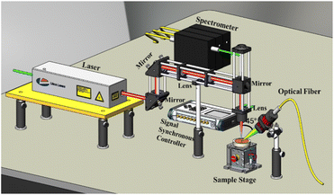 | ||
| Fig. 1 Experimental setup (including laser, optical system, sample stage, spectrometer, signal synchronous controller, and software system). | ||
In the experiment, the frequency of laser beam emission is 1 Hz, the integration time is 1.2 ms, the energy of a signal laser pulse is 80 mJ, and the time interval between the laser and the spectrometer is 2.81 μs. The influence of bremsstrahlung is minimal and the spectral signal is the best by adjusting the above experiment parameter.
2.2 Sample preparation
The experimental samples were sixteen kinds of natural rock, which were divided into nine types according to provenances and lithology. Among them, three types (SY1, SY2 and SY3) are mined from the Dajianggang area in Shuangyang, which are different types of sandstone. The other six types (DX1, DX2, DX3, DX4, DX5 and DX6) are mined from the Chaihe area in Daxing'anling, including different types of andesite and sandstone. Detailed sample classification information is shown in Table 1.| No. | Lithology | Provenance | Category |
|---|---|---|---|
| 1 | Pebbly sandstone | Dajianggang area | SY1 |
| 2 | Sandstone | Dajianggang area | SY2 |
| 3 | Greywacke | Dajianggang area | SY3 |
| 4 | Andesite | Chaihe area | DX1 |
| 5 | Andesite | Chaihe area | DX1 |
| 6 | Andesite | Chaihe area | DX1 |
| 7 | Andesite | Chaihe area | DX1 |
| 8 | Andesite | Chaihe area | DX1 |
| 9 | Coarse sandstone | Chaihe area | DX2 |
| 10 | Coarse sandstone | Chaihe area | DX2 |
| 11 | Coarse sandstone | Chaihe area | DX2 |
| 12 | Pebbled-medium–coarse sandstone | Chaihe area | DX3 |
| 13 | Sandstone | Chaihe area | DX4 |
| 14 | Medium–coarse sandstone | Chaihe area | DX5 |
| 15 | Medium–coarse sandstone | Chaihe area | DX5 |
| 16 | Medium sandstone | Chaihe area | DX6 |
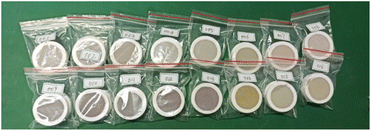
The samples used for spectral data acquisition are shown in Fig. 2. At first, the mined rock samples were treated into uniform rock powder with a grinding machine. Then, the powder pressing machine (BP-1, China) laminated them into thin cylindrical with a diameter of 40 mm and a height of 6.25 mm at a pressure of 30 MPa. Borate powder was used as a binder around and on the bottom of the rock powder to obtain better sample materials for the LIBS experiment.28 After testing on the experimental platform, the spectral data is better.
2.3 Data set establishment
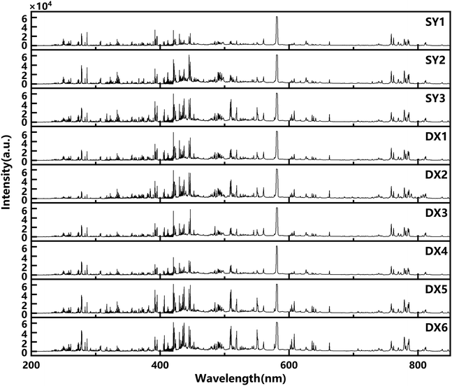
In the experiment, 100 groups of data were collected from any ten non-overlapping sampling points on the surface of each rock sample. And every twenty groups of data were averaged so that five groups of representative spectral data were obtained from each sampling point. They were used to carry out the data analysis in the experiment. The full spectra of the nine types of rock samples collected are shown in Fig. 3. In the establishment process of the training set and the testing set, the spectral data of five sampling points were randomly selected for each type of rock sample. 225 groups of data were used as the final experimental data to discriminate the provenances and lithology of the rocks. The spectral data were divided into the training set and testing set with a ratio of six to four. Hence, there are 135 groups of data constituting the training set to train the discrimination model, and 90 groups of data constituting the testing set to test the performance of the model.2.4 Model evaluation
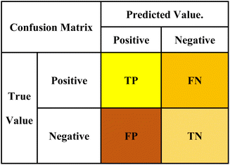
The methods used to evaluate classification models commonly include confusion matrix, ROC curve, and AUC area.29 The confusion matrix was adopted in this paper. The confusion matrix, also known as the error matrix, is essentially a table composed of the number of correct and wrong classifications. As shown in Fig. 4, the dichotomy problem is taken as an example. The results of the sample judged by the model to be evaluated are 0 or 1, namely positive or negative, which are called the predicted value. The actual positive and negative values of samples can be obtained according to the actual situation, which is called the true value. Compared the predicted value with the true value, four indicators can be captured: True Positive (TP) indicates the number that the true value is positive and the predicted value is positive judged by the mode, False Positive (FP) indicates the number that the true value is negative and the predicted value is positive; for the same reason, True Negative (TN) indicates the number that the real value is negative and the predicted value is negative, False Negative (FN) indicates the number that the true value is positive and the predicted value is negative.According to the indicator shown in the confusion matrix, statistical values such as accuracy, precision, recall and others can be calculated. They are secondary indicators of the model. In addition to this, the confusion matrix also has a third-level indicator called the F1 score. The performance of the discrimination model can be evaluated by comparing the advantages and disadvantages of the statistical values.
In this paper, we calculated the accuracy, precision, recall and F1 score of the model through the confusion matrix to evaluate the analysis performance of the established model. The calculation method is as follows:
(a) Accuracy: the proportion of correct results predicted by the model in the total sample number.
(b) Precision: the proportion of correct results predicted by the model in the predicted value of positive.
(c) Recall: the proportion of correct results predicted by the model in the real value of positive.
(d) F1 score: a combination of precision and recall.
The higher the above value, the better the performance of the model.
3. Results and discussion
3.1 Model of provenance discrimination based on preprocessing methods
At first, three algorithms including PLS, KNN, and RF were used to establish models.30–32 The models discriminate the provenances of the rock samples respectively. The original full spectra of rock samples that had been divided into the training set and testing set before were applied to establish the three models respectively. The prediction results of the three models are shown in Fig. 5.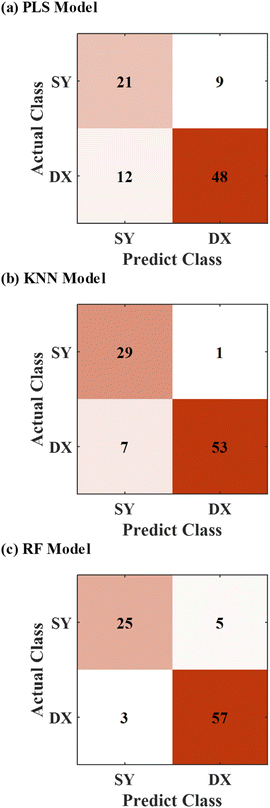 | ||
| Fig. 5 Prediction results of PLS model (a), KNN model (b), and RF model (c) established by the original full spectra. | ||
The first figure in Fig. 5 presented the results predicted by the PLS model. Nine groups of data of the rock samples from the Dajianggang area and twelve groups of data of the rock samples from the Chaihe area were put into the wrong category, with a final accuracy of 76.67%. The prediction results of the KNN model were shown in Fig. 5(b). One group and seven groups of data were incorrectly discriminated respectively in two provenances, and the accuracy is 91.11%. The RF model was used for discrimination, and the prediction results were shown in Fig. 5(c). Among ninety groups of data in the testing set, five groups and three groups were discriminated into the incorrect category. The RF model gained a prediction accuracy of 91.11%. As for the data of original full spectra, the KNN and RF models had the same performance on the provenance discrimination among the three models.
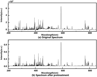
There are background noise interference and system random error in data acquisition of the LIBS spectrum, which leads to the lower classification accuracy of the model.33 Before analysing, the spectral data need to be pretreated with preprocessing methods such as baseline correction, smoothing handling, normalization, scattering correction, and others.34 The common methods used to pretreat data include wavelet transform, derivative, multivariate scattering correction, normalization, etc.35–37 In this work, the outliers were first processed, that is, the spectral lines whose intensity value was less than 0 in the spectrum were replaced by 0. Then, after analysing the original full spectrum of rock samples in Fig. 3, the third-order Savitzky–Golay Smoothing Filter was used to improve the spectral smoothness by moving a window with a width of 61. And Baseline Estimation And Denoising with Sparsity (BEADS) eliminates the spectral baseline drift phenomenon by fitting the baseline. Finally, the spectrum was uniformed dimension by Min–Max Scaling. Min–Max Scaling normalizes the spectrum to between 0 and 1. The comparison of the original spectrum and the spectrum after pretreatment is shown in Fig. 6.
We used the data of full spectra that were pretreated by the above preprocessing methods to establish three models (PLS, KNN, and RF) again. The prediction results of the models are shown in Fig. 7. In contrast to the models established by the data of the original full spectra (Fig. 5), all of the models established by the data treated by the preprocessing methods had obvious improvements in discrimination performance. The accuracies of the three models respectively are 94.44%, 93.33% and 96.67%.
 | ||
| Fig. 7 Prediction results of PLS model (a), KNN model (b), and RF model (c) established by the pretreated full spectra. | ||
The six models were established to verify the effectiveness of the preprocessing methods to improve the classification accuracy of models. The statistical results for the prediction performance are presented in Table 2. The results showed that LIBS combined with machine learning can be used to discriminate the different rock origins and the preprocessing methods can effectively improve the prediction performance of the model. The performance of the RF model based on preprocessing methods was the best among the six models, and the accuracy reached 96.67%. Only three groups of data were incorrectly discriminated. In the following experiments, we focus on optimizing the RF model to obtain better discrimination performance. The full spectra of rock samples were used to train and test the models, which is still inadequate. Because some unimportant spectral lines affect the establishment of the model, the prediction performance of the model will be weakened. We decided to use the method of variable importance to extract important spectral lines.
| Algorithm | Preprocessing methodsa | Wrong number | Correct number | Accuracy |
|---|---|---|---|---|
| a The preprocessing methods include outlier elimination, Savitzky–Golay Smoothing Filter, Baseline Estimation And Denoising with Sparsity (BEADS), and Min–Max Scaling. | ||||
| PLS | 21 | 69 | 76.67% | |
| PLS | ✓ | 5 | 85 | 94.44% |
| KNN | 8 | 82 | 91.11% | |
| KNN | ✓ | 6 | 84 | 93.33% |
| RF | 8 | 82 | 91.11% | |
| RF | ✓ | 3 | 82 | 96.67% |
3.2 Model of provenance discrimination based on variable selection
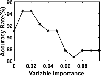
LIBS spectrum is characterized by a large amount of data and complexity. In this research, each group of spectral data has 6144 spectral lines. The important variables of the spectrum have easily interfered with other ignorable variables in the analysis process. In order to optimize the RF model for rock discrimination, the variable selection method based on the random forest was studied. Random Forest can rank variable factors by calculating the important value of the variable. There are three approaches to measuring the value of variable importance: Shapley Variable Importance, Permutation Variable Importance and Gini Variable Importance.38 In this work, Gini Variable Importance was calculated to rank the important variable of spectral data. The weighted sum of the decreases in impurity for all the nodes is the Gini Variable Importance.Then, the spectral data was selected as input according to the variable importance of different thresholds to establish the RF model for the discrimination of the rock provenances. The prediction accuracies of each established RF models for the testing set were obtained, as shown in Fig. 8. The optimal prediction accuracy of the RF model is 94.44% when the threshold of variable importance is 0.01 or 0.02.
We employed the case that the threshold of variable importance is 0.02. In this case, the importance value of the spectral variable is shown in Fig. 9(b). The black arrows indicate elements with a high value of the variable importance, which means that these elements have a great impact on the performance of the model in the process of rock provenance discrimination. Spectra with high intensity are shown in Fig. 9(a). Meanwhile, the major elements, the ones that are more abundant in the rock, are indicated with red arrows. Comparing the two stems in Fig. 9, the contents of Mg, K and Mn are not only high but also obviously different in samples from different provenances. However, the contents of other elements in the samples are not high, but they have high variable importance values. The discrimination of the provenance is based on the difference in the element contents. Most of these elements are less in rocks and only a few belong to the major elements. The content of major elements does not change much in the process of rock formation. But due to the influence of different geological processes in different provenances, the content difference of trace elements in rocks increases gradually.
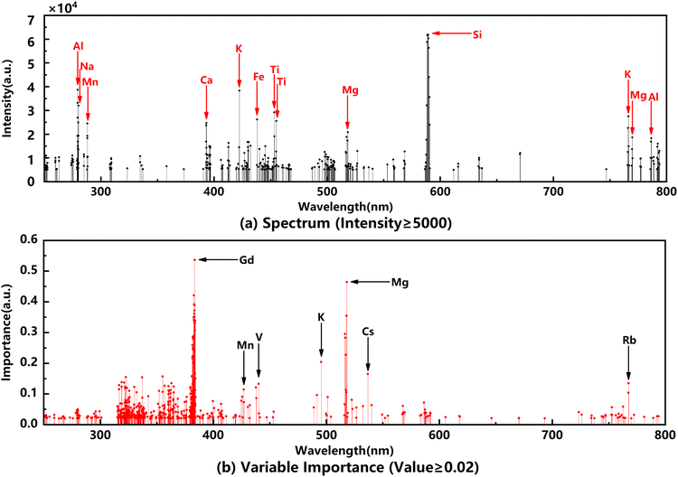 | ||
| Fig. 9 The spectrum (a) with the main elements (red arrows) and the importance value (b) with the elements of high importance variable values (black arrows). | ||
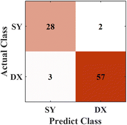
The optimal performance of the model based on the variable importance for the provenance discrimination is shown in Fig. 10. There are three groups of the Chaihe area and two groups of the Dajianggang area incorrectly discriminated. Compared with the RF model established with the original full spectrum, the prediction accuracy of the RF model increased from 91.11% to 94.44%. The experimental results show that the method of variable importance selection can be used to improve the discrimination performance of the model for the rock provenances.
The experiments proved that both the preprocessing methods and the variable importance selection have a positive effect on the discrimination performance of the model for rock provenances. To further verify the model, the preprocessing methods and variable importance selection with a threshold of 0.2 were treated with spectral data simultaneously, then we tested the established model. The prediction results of the model are shown in Fig. 11. Only two groups of data in the testing set were incorrectly discriminated, both of which originated from the Dajianggang area. The accuracy of this new RF model reaches 97.78%, which is better than that of all the previous models.
 | ||
| Fig. 11 Predicted results of the model with preprocessing methods and variable importance selection. | ||
In this experiment, four RF models have been established with different spectral data including the data of the original full spectrum, the spectral data with preprocessing methods, the spectral data with variable importance selection, and the spectral data with preprocessing methods and variable importance selection. The discrimination performances of the four models for 90 groups of data in the testing set are shown in Table 3. The results show that the RF model established by the data of the spectrum with preprocessing methods and variable importance selection exhibited optimum performance, and its accuracy reaches 97.78%. Among the four models, its possibility of error is the lowest. Only two groups of data were discriminated into the incorrect type. Compared with the other RF models, the classification accuracy of the model established by such data has been significantly elevated.
| Model | Preprocess methods | Variable importance | Wrong number | Correct number | Accuracy |
|---|---|---|---|---|---|
| RF | 8 | 82 | 91.11% | ||
| RF | ✓ | 3 | 87 | 96.67% | |
| RF | ✓ | 5 | 85 | 94.44% | |
| RF | ✓ | ✓ | 2 | 88 | 97.78% |
In order to better compare the performance of the four models, the precision, recall and F1 score of the predicted results were also calculated, as shown in Table 4. The results again prove that the pretreatment methods and the selection of important variables can effectively improve the classification performance of the model. And the performance of the model optimized by the two methods is optimal. Beyond that, the discrimination performance of rock samples from the Chaihe area is generally better than that from the Dajianggang area. The reason is related to the quantity and type of rock samples in the two areas. In training set data, there are 90 groups of data of rock samples from the Chaihe area constituted of six types of rock samples. However, in the training set of the Dajianggang area, only 45 groups of rock sample data were composed, all of which are sandstone. For the Dajianggang area, the experimental rock samples have the characteristics of a small amount of data and a single type. Hence, the RF model presented better discrimination performance to discriminate the rock samples from the Chaihe area.
| Model | Preprocess methods | Variable importance | SY | DX | ||||
|---|---|---|---|---|---|---|---|---|
| Precision | Recall | F 1 score | Precision | Recall | F 1 score | |||
| RF | 89.29% | 83.33% | 86.21% | 91.94% | 95.00% | 93.44% | ||
| RF | ✓ | 100% | 90.00% | 94.74% | 95.24% | 100% | 97.56% | |
| RF | ✓ | 90.32% | 90.33% | 91.80% | 96.61% | 95.00% | 95.80% | |
| RF | ✓ | ✓ | 100% | 90.33% | 96.55% | 96.77% | 100% | 98.36% |
3.3 Model of lithology discrimination
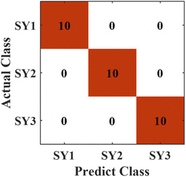
The optimized RF model was used to identify the provenances of rock samples, and excellent discrimination performance was obtained. In order to further verify the feasibility of the RF model for the analysis of rock samples from two provenances, the RF algorithm was used to discriminate the lithology of the rock samples from the two provenances respectively.The reason why the three types of rocks from the Dajianggang area are easily discriminated mainly is that there are obvious differences in the element among the three types of sandstone. Their diversities were reflected as different characteristic peaks in the spectrum. According to the properties of the three kinds of rock, pebbly sandstone and greywacke contain other chemical compositions that are different from those of sandstone. On the basis of sandstone, pebbly sandstones have components of gravel with larger granularity than sandstone. The elements contained in the gravel are related to the geological structure of the parent rock region and geological processes during rock formation, such as weathering, biological action, external force handling, and so on. Greywacke is more complex than sandstone in composition and has a higher content of special elements. Therefore, the RF model can distinguish the three types of rocks in the Dajianggang area with excellent discrimination performance.
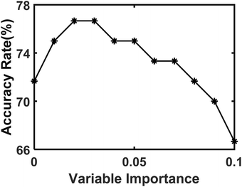 | ||
| Fig. 13 Prediction accuracies of different thresholds of variable importance for lithology in Chaihe area. | ||
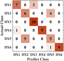
The pebbly-medium–coarse sandstone can be completely discriminated from six types of rock samples from Chaihe area. The reason is mainly related to the gravel in the pebbly-medium–coarse sandstone. There is a slight confusion between andesite and sandstone, which is mainly affected by parent rocks. Different rocks from the same provenance may be similar in the contents of the characteristic elements. In this work, the natural rock is ground into powder. Medium sandstone and coarse sandstone are similar in composition and are often distinguished according to the particle size of the rock in practice. The particle size of medium sandstone and coarse sandstone is between 0.25–0.5 mm and 0.5–2 mm, respectively. The rock samples in this experiment had been ground, the particle size of the rock had been destroyed, and the difference between them is much harder to distinguish. So there would be varying degrees of confusion when discriminating among four types of sandstones.
LIBS technology combined with the RF algorithm was used to analyse the lithology of rock samples from two provenances respectively. The classification accuracy of rock samples from the Dajianggang area was 100%, while that of the Chaihe area was only 76.67%. The experimental results indicated that the model can better discriminate the rock samples with distinct content characteristics. In essence, the RF algorithm is based on the element content of samples to discriminate, so the performance of the model for sandstone with different particle sizes is poor, such as medium sandstone and coarse sandstone.
4. Conclusions
In this paper, LIBS technology combined with machine learning methods was used to discriminate the provenance and the lithology of rock samples. The six models were established with three algorithms including PLS, KNN, and RF to demonstrate the availability of preprocessing methods. The RF model based on the pretreated data gained the optimum discrimination performance. In order to improve the performance of the model, we used four different methods to deal with spectrum data. Compared to the results of the four models, the model established with the data of preprocessing methods and variable importance selection gained the highest accuracy of 97.78%. Then, the RF algorithm was also used to discriminate the lithology of rock samples from two areas. The accuracy of the model established only with pretreated data reached 100%. However, when analysing the lithology of rock samples from the Chaihe area, the accuracy of the optimum model established with the data of preprocessing methods and variable importance selection reached 76.67%. And the results presented varying degrees of confusion. The experimental results showed that the RF algorithm can be used to discriminate the provenance of rocks from different areas and the lithology of rocks with distinct content characteristics. And the LIBS technology combined with the RF algorithm is not suitable for the discrimination of sandstone with different particle sizes.Conflicts of interest
There are no conflicts to declare.Acknowledgements
The authors are grateful to the National Nature Science Foundation of China [Grant No. 62275099], the National Nature Science Foundation of China [Grant No. 41872234], Science and Technology Research Project of the Education Department of Jilin Province (No. JJKH20220993KJ).Notes and references
- K. Ueki, H. Hino and T. Kuwatani, Geochem., Geophys., Geosyst., 2018, 19(4), 1327–1347 CrossRef.
- Q. M. Pei, C. H. Li, S. T. Zhang, H. Zou, Y. Liang, L. Wang, S. L. Li and H. W. Cao, Ore Geol. Rev., 2022, 142, 104708 CrossRef.
- M. A. Chen and B. D. Kocar, J. Synchrotron Radiat., 2021, 28, 461–471 CrossRef CAS PubMed.
- A. Sharma, A. Muyskens, J. Guinness, M. L. Polizzotto, M. Fuentes, R. V. Tappero, Yc. K. Chen-Wiegart, J. Thieme, G. J. Williams, A. S. Acerbo and D. Hesterberg, J. Synchrotron Radiat., 2020, 26, 1967–1979 CrossRef PubMed.
- G. Aertgeerts, J. P. Lorand, C. Monnier and C. La, Lithos, 2018, 314, 100–118 CrossRef.
- W. T. Bu, M. Gu, X. T. Ding, Y. Y. Ni, X. P. Shao, X. M. Liu, C. T. Yang and S. Hu, J. Anal. At. Spectrom., 2021, 36(11), 2330–2337 RSC.
- G. H. Gao, J. Cao, K. Hu, T. W. Xu, H. A. Zhang and Y. X. Zhang, Energy Fuels, 2021, 35(2), 1234–1247 CrossRef CAS.
- S. N. Shilobreeva, J. Anal. Chem., 2018, 72(14), 1355–1368 CrossRef.
- L. B. Guo, D. Zhang, L. X. Sun, S. C. Yao, L. Zhang, Z. Z. Wang, Q. Q. Wang, H. B. Ding, Y. Lu, Z. Y. Hou and Z. Wang, Front. Phys., 2021, 16(2), 45–69 Search PubMed.
- X. J. Xu, C. Sun, Y. Q. Zhang, Z. Q. Yue, S. Shabbir, L. Zou, F. Y. Chen, L. Wang and J. Yu, J. Anal. At. Spectrom., 2021, 37(2), 317–329 RSC.
- V. Balaram, Geol. J., 2020, 56(5), 2300–2359 CrossRef.
- M. Kuzmanovic, A. Stancalie, D. Milovanovic, A. Staicu, L. J. Damjanovic-Vasilic, D. Rankovic and J. Savovic, Opt. Laser Technol., 2021, 134, 106599 CrossRef CAS.
- Y. Zhang, T. L. Zhang and H. Li, Spectrochim. Acta, Part B, 2021, 181, 106218 CrossRef CAS.
- Y. C. Liu, B. B. Zhou, W. L. Wang, J. D. Shen, W. P. Kou, Z. B. Li, D. Zhang, L. B. Guo, C. Lau and J. Lu, ACS Sens., 2022, 7(5), 1381–1389 CrossRef CAS PubMed.
- P. Vanraes and A. Bogaerts, Spectrochim. Acta, Part B, 2021, 179, 106091 CrossRef CAS.
- C. Wang, J. Wang, J. Wang, H. Du and J. H. Wang, Laser Phys., 2021, 31, 035601 CrossRef CAS.
- C. Fabre, Spectrochim. Acta, Part B, 2020, 166, 105799 CrossRef CAS.
- P. A. Defnet, M. A. Wise, R. S. Harmon, R. R. Hark and K. Hilferding, Minerals, 2021, 11, 705 CrossRef CAS.
- D. Han, Y. J. Joe, J. S. Ryu, T. Unno, G. Kim, M. Yamamoto, K. Park, H. G. Hur, J. H. Lee and S. I. Nam, Spectrochim. Acta, Part B, 2018, 146, 84–92 CrossRef CAS.
- Y. Ding, W. Zhang, X. Q. Zhao, L. W. Zhang and F. Yan, J. Anal. At. Spectrom., 2020, 35(6), 1131–1138 RSC.
- T. T. Chen, T. L. Zhang and H. Li, TrAC, Trends Anal. Chem., 2021, 133, 116113 CrossRef.
- W. J. Xu, C. Sun, Y. Q. Zhang, Z. Q. Yue, S. Shabbir, L. Zou, F. Y. Chen, L. Wang and J. Yu, J. Anal. At. Spectrom., 2021, 37(2), 317–329 RSC.
- H. W. Ji, Y. Ding, L. W. Zhang, Y. W. Hu and X. C. Zhong, Appl. Spectrosc. Rev., 2021, 56(3), 193–220 CrossRef CAS.
- M. G. Yan, X. Z. Dong, Y. Li, Y. Zhang and Y. F. Bi, Spectrosc. Spectral Anal., 2018, 38(6), 1874–1879 CAS.
- L. W. Sheng, T. L. Zhang, G. H. Niu, K. Wang, H. S. Tang, Y. X. Duan and H. Li, J. Anal. At. Spectrom., 2015, 30(2), 453–458 RSC.
- H. X. Yang, H. B. Fu, H. D. Wang, J. W. Jia, M. W. Sigrist and F. Z. Dong, Chin. Phys. B, 2016, 25(6), 065201 CrossRef.
- C. Wang, X. M. Zhang, X. P. Zhu, W. F. Luo and J. Shan, Acta Photonica Sin., 2019, 48(10), 164–172 Search PubMed.
- M. C. Zuma, J. Lakkakula and N. Mketo, Appl. Spectrosc. Rev., 2021, 57(5), 353–377 CrossRef.
- L. L. Xu and D. X. Chi, Computer Engineering and Applications, 2020, 56(24), 12–27 Search PubMed.
- M. R. Dong, L. P. Wei, J. J. Gonzalez, D. Oropeza, J. Chirinos, X. L. Mao, J. D. Lu and R. E. Russo, Anal. Chem., 2020, 92(10), 7003–7010 CrossRef CAS PubMed.
- T. F. Boucher, M. V. Ozanne, M. L. Carmosino, M. D. Dyar, S. Mahadevan, E. A. Breves, K. H. Lepore and S. M. Clegg, Spectrochim. Acta, Part B, 2015, 107, 1–10 CrossRef CAS.
- P. Janovszky, K. Jancsek, D. J. Palasti, J. Kopniczky, B. Hopp, T. M. Toth and G. Galbacs, J. Anal. At. Spectrom., 2021, 36(4), 813–823 RSC.
- T. K. Sahoo, A. Negi and M. K. Gundawar, 2015 International Conference on Advances in Computing, Communications and Informatics, Aluva, Aug., 2015 Search PubMed.
- C. Y. Pan, J. He, G. Q. Wang, X. W. Du, Y. B. Liu and Y. H. Su, Plasma Sci. Technol., 2019, 21(3), 034012 CrossRef CAS.
- V. Tafintseva, T. A. Lintvedt, J. H. Solheim, B. Zimmermann, H. U. Rehman, V. Virtanen, R. Shaikh, E. Nippolainen, I. Afara, S. Saarakkala, L. Rieppo, P. Krebs, P. Fomina, B. Mizaikoff and A. Kohler, Molecules, 2022, 27, 3 CrossRef PubMed.
- K. J. Sorauf, A. J. R. Bauer, A. W. Miziolek and F. C. De Lucia, Next-Generation Spectroscopic Technologies VIII, Baltimore, Apr., 2015 Search PubMed.
- N. H. Cheung, J. Anal. At. Spectrom., 2019, 34(3), 616–622 RSC.
- K. Wei, Q. Q. Wang, G. E. Teng, X. J. Xu, Z. F. Zhao and G. Y. Chen, Appl. Sci., 2022, 12(10), 4981 CrossRef CAS.
| This journal is © The Royal Society of Chemistry 2023 |

