
 Open Access Article
 This Open Access Article is licensed under a
 Creative Commons Attribution 3.0 Unported Licence
Environmentally benign fabrication of superparamagnetic and photoluminescent Ce,Tb-codoped Fe3O4-gluconate nanocrystals from low-quality iron ore intended for wastewater treatment†
Utsav
Sengupta
 a,
Muthaimanoj
Periyasamy
b,
Sudipta
Mukhopadhyay
b and
Arik
Kar
*a
a,
Muthaimanoj
Periyasamy
b,
Sudipta
Mukhopadhyay
b and
Arik
Kar
*a
aDepartment of Chemistry, Indian Institute of Engineering Science and Technology, Shibpur, Howrah 711 103, India. E-mail: akar@chem.iiests.ac.in; Tel: +0091 8334845357
bDepartment of Mining Engineering, Indian Institute of Engineering Science and Technology, Shibpur, Howrah 711 103, India
First published on 9th October 2023
Abstract
At present, wastewater treatment is a fundamental ecological problem since contaminated organics, such as dyes, stand as a foremost and rising cause of water pollution. Accordingly, legislation directed toward ensuring the elimination of toxic dyes from wastewater is becoming ever more rigorous, making the progress of more effective nanomaterials for degrading toxic dyes a critical challenge for chemists. A capable technique to address this problem utilizes metal ion-doped semiconductors to catalytically photodegrade the stable bonds in these dye molecules. Despite extensive research in this area, the invention of an efficient doped semiconductor system remains a key challenge. Herein, we have advanced the previous study by designing a fluorescent-superparamagnetic-photocatalytic Ce,Tb-codoped Fe3O4 nanocrystals with an amorphous carbon coating via an unsophisticated single-pot D-glucose mediated hydrothermal reduction method using a single iron precursor (FeCl3·6H2O) obtained from gathered iron ore tailings- a mining waste that characteristically symbolizes a major environmental hazard. Such trifunctional nanocrystal formations were verified using X-ray diffraction (XRD), FTIR spectroscopy, X-ray photoelectron spectroscopy (XPS), Brunauer–Emmett–Teller (BET) surface area analysis, and transmission electron microscopy (TEM) imaging. XPS and XRD analyses confirmed the efficient doping of lanthanide ions into the Fe3O4 host lattice. Photoluminescence (PL) spectra showed that the doped nanocrystals with a precise dopant ratio displayed a strong cyan light emission. Furthermore, time-correlated single-photon counting (TCSPC) measurements indicated how the dopant percent variation in Fe3O4 influenced their corresponding average lifetime values. The magnetization measurements demonstrated the superparamagnetic behavior with variated magnetic saturation values, which were established to be dependent on the doping effect. Samples with an appropriate doping ratio were established to be more efficient for the photodecomposition of Rhodamine B under visible light irradiation with remarkable recyclability and structural stability. Such trifunctional nanocrystals may find many biomedical applications, such as cancer detection and drug delivery, and the technique we used can be extended to the synthesis of other nanomaterials based on lanthanide ion-doped materials and metal oxides.
1. Introduction
Nanomaterials have recently attracted enormous attention due to their properties being different from those of their bulk counterparts.1–4 In particular, magnetic, optical, and photocatalytic nanomaterials were intensively pursued owing to their extensive applications. Magnetic nanoparticles (NPs) have opened up huge prospects in drug targeting,5,6 while fluorescent NPs have attracted more consideration in the field of biological labeling,7,8 and photocatalytic NPs have been applied to health and environmental problems associated with water pollution.9 Recently, scientists have been involved in combining the magnetic, fluorescent, and photocatalytic NPs into innovative ‘‘three-in-one’’ trifunctional NPs,10,11 which have been difficult to obtain.Magnetite (Fe3O4) has become one of the most accepted and widely studied semiconductors that can exhibit both n- and p-type semiconductor behaviors with a narrow band gap (0.1 eV) for the bulk phase.12,13 The narrow band gap energy allows for the quick recombination of the photo-generated electrons and holes, which considerably limits the creation of reactive oxygen species.14 So, the tuning of the Fe3O4 particle size to an ultra-nanoscale size is highly desirable for increasing their band gap, as well as restricting their rapid electron–hole recombination.9 So far, the strategies developed to adapt the magnetic, optical, and photocatalytic properties of Fe3O4 are metal ion doping15,16 or heterostructure design17,18 or defect engineering.19,20 Among them, metal ion doping has attracted much attention for adapting the magnetic, optical, and photocatalytic properties.21,22 Accordingly, various synthetic methods have been reported in the literature to manufacture metal ion-doped Fe3O4 nanoparticles with the desired physical and chemical properties.23,24 However, most of the formerly reported synthetic methods involve a complicated and expensive equipment setup. Notably, the organic templates-assisted hydrothermal method has gained considerable attention compared to other synthetic methods.25,26
Among various metal ions, lanthanide (Ln) ions are one of the attractive classes of dopants that hold distinctive optical and magnetic properties associated with their f-electronic configurations.27,28 Ln-doped Fe3O4 NPs were selected as optical materials because of their striking features, such as the large Stokes shifts, high resistance to photobleaching, blinking, and photochemical degradation.29,30 Previously, the co-precipitation and/or reverse micelle method was exploited for preparing Ln-doped Fe3O4 NPs.31,32 However, several concerns have been identified with the previously mentioned methods, such as the difficulty in controlling the particle size and achieving a monodisperse size distribution.33 Therefore, a few alternative preparative approaches are highly desirable to overcome this issue.
Many studies have spotlighted the production of Ln-doped Fe3O4 NPs using harmless and environmentally friendly precursor materials. Particularly, the exploitation of metallurgical waste obtained from mining industries for the synthesis of Fe3O4 NPs has achieved considerable attention. In the case of iron ore processing industries, tons of mining wastes have been excreted each year, resulting in the pollution of the air atmosphere and different water bodies such as lakes, dams, ponds, rivers, and others. The key waste component here is the iron ore tailings (IOTs). IOT is a solid waste formed during the beneficiation process of iron ore concentrate. Although IOTs are extremely toxic materials, they can be treated for the design of various porous materials, battery and fuel cells, and others.34 So, it is vital to convert IOTs to some eco-friendly products that can be valuable for numerous productive applications. There are already a few techniques that have been reported in the literature for iron extraction from IOTs, such as leaching,35 suspension magnetization roasting (SMR),36 and others.
This contribution presents a cost-effective and bio-friendly original synthetic approach for designing super-efficient and highly recyclable cerium (Ce) and terbium (Tb)-doped Fe3O4 NPs via a low temperature hydrothermal technique by using Fe3+ as the sole metal precursor obtained from the magnetically less effective and more toxic starting material IOTs via the leaching process. The structure, morphology, and optical properties of the as-synthesized samples were investigated by XRD, FTIR, XPS, TEM, UV-vis spectroscopy, N2 adsorption/desorption, and TGA analysis. Photoluminescence (PL) spectra confirmed that the doped sample displayed a strong cyan light emission. The magnetic measurements demonstrate the superparamagnetic behavior, which is found to be dependent on the doping effect. In addition, the catalyst recovery and recyclability tests have been performed to establish the photocatalyst's stability. A feasible photocatalytic mechanism has been proposed that seeks to relate the doping effect with the photocatalytic properties. In summary, the main focus of this article can be represented by a cycle diagram (Fig. 1a), which points out how harmful mining wastes can be recycled for environmental remediation. Another diagram (Fig. 1b) represents the production of an eco-friendly material from an eco-hazard material, and its utilization for removing some eco-pollutants for purifying the contaminated water resources.
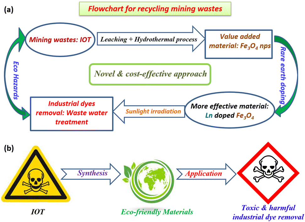 | ||
| Fig. 1 (a) Cyclic pathway for utilizing the mining wastes for environmentally friendly applications. (b) One-arrow diagram for the conversion of an eco-hazard to an eco-friendly material and its uses. | ||
2. Experimental section
2.1. General synthetic procedures
The collection of iron ore tailings (IOTs) was performed in the tailing dams of the Donimalai iron ore mines of the National Mineral Development Corporation (NMDC), India (Location: Bellary-Hospet sector, Karnataka, India). The further treatment process of IOTs and its selective leaching method are described comprehensively in the ESI† file (Sections 1.1 and 1.2, ESI†). Here, Table 1 illustrates the chemical composition and the mineral phases of the IOTs executed by micro X-ray fluorescence spectroscopy analysis (μ-XRF).| Oxides of the primary and trace elements | Fe (total) | Al2O3 | SiO2 | MgO | CaO | MnO | TiO2 | Cr2O3 | V2O5 | K2O | P2O5 | SO3 |
|---|---|---|---|---|---|---|---|---|---|---|---|---|
| Weight (%) | 71.38 | 10.77 | 16.64 | 0.31 | 0.32 | 0.07 | 0.32 | 0.02 | 0.02 | 0.16 | 0.22 | 0.03 |
All other chemical ingredients like solvents [HPLC water (Millipore) and absolute ethanol], acid (concentrated HCl), and dextrose were purchased from Merck India. Cerium(III) nitrate hexahydrate and terbium(III) nitrate pentahydrate were purchased from Sigma Aldrich. Liquid ammonia (25%) was purchased from Fisher Scientific Ltd. All of the above chemicals were used without further purification.
2.2. Preparation of pure Fe3O4/C nanocomposites
Previously, we have reported the iron ore tailings (IOTs) purification process to obtain the hydrolysate solution (FeCl3·6H2O), and the subsequent hydrothermal reduction process to obtain carbon-coated magnetite nanocomposites.9,35 In brief, a certain amount of IOTs (collected from iron ore mining wastes) are boiled with concentrated HCl (120 °C for 6 h) and filtered to get the purified hydrolysate solution, i.e., FeCl3·6H2O (more precisely, it is called leachate solution). After that, 2 g of dextrose (10 mmol) was added as a mild reducing agent to 25 mL of 5 mM hydrolysate solution. The obtained acidic mixture was further made to be moderately highly basic (pH 10–11) by using ∼50 mL (in excess) 25% liquid ammonia solution. After vigorously stirring for 30 min, the deep brown mixture was transferred to a 120 mL hydrothermal reactor (Teflon-made inner container and outer surface built of stainless steel) and tightly sealed. The reactor was then heated in an autoclave chamber at 200 °C for 24 h. After the reaction was completed, the hot hydrothermal reactor was cooled automatically to room temperature. Then, the final product was obtained by washing it a couple of times with distilled water (3 × 25 mL) and absolute ethanol (3 × 25 mL), respectively. The obtained product was finally dried in a hot air oven at 70 °C for 6 h to obtain the dark brown amorphous powder. The synthetic scheme is given in Fig. 2. | ||
| Fig. 2 Synthesis route in a continuous flow chart diagram. | ||
2.3. Preparation of Ce–Tb doped Fe3O4/C nanocomposites at various dopant ratios
The synthesis pathway of the hydrolysate mixture is the same as above. Herein, to synthesize the Ln-doped samples, Ce(NO3)3·6H2O, and Tb(NO3)3·5H2O salts are added to the acidic mixture before adding D-glucose. As both the lanthanide salts are soluble in water, they easily dissolve in the acidic solution. The remaining process was the same as that described above. Here, the prepared samples are slightly blackish brown compared to the pure Fe3O4, and also more crystalline as observed by the naked eye (Fig. 2). By altering the weight percentages of the dopants (Ce and Tb), various doping ratios were obtained. Here, we have prepared 3 doped samples and they are – 1% Ce3+ + 0.5% Tb3+ (abbreviated as – ‘1Ce–0.5Tb@G24’), 1% Ce3+ + 1% Tb3+ (abbreviated as – ‘1Ce–1Tb@G24’), and 0.5% Ce3+ + 1% Tb3+ doped Fe3O4/C (abbreviated as – ‘0.5Ce-1Tb@G24’), and one pure Fe3O4, which is abbreviated as ‘G24’. All have different amounts of amorphous carbon coating. The synthesis process is summarized in a flow chart diagram of the sample preparation (Fig. 2).3. Characterization
3.1. X-ray diffraction (XRD) analysis
XRD profiles of both pure and doped samples were recorded using Ni-filtered Cu Kα (λ = 0.154 nm) from a highly stabilized and automated PAN-analytical X-ray generator at 35 kV and 25 mA. The X-ray generator was coupled with a PW3071/60 bracket goniometer for sample mounting. Step-scan data (step size 0.02° 2θ, counting time 2 s per step) were recorded for 20°–80° 2θ.3.2. Transmission electron microscopy (TEM) analysis
Fe3O4 nanoparticles were prepared for TEM analysis by sonication in EtOH before being drop-cast onto a holey carbon copper TEM grid (Agar Scientific). Preliminary sample analysis used a FEI Philips Tecnai 20 (200 KeV) with a 70 μm objective aperture, CCD camera, and 200 KeV source. For more detailed interrogation, high-resolution transmission electron microscopy (HR-TEM, JEOL-JSM2010) is used for the microscopic characterization of the Fe3O4 nanoparticles.3.3. X-ray photoelectron spectroscopy (XPS)
XPS measurements were carried out using a ThermoScientific K-Alpha system. The spectra were recorded using a focused monochromatized Mg Kα X-ray source (1253.6 eV) and Al Kα X-ray source (1486.8 eV). The binding energy was calibrated internally based on the C 1s line position.3.4. UV-diffuse reflectance spectroscopy (UV-DRS)
Data were collected on a Varian Cary-50 UV-Vis spectrophotometer with a Harrick Video-Barrelino diffuse reflectance probe.3.5. FTIR spectroscopy
The Fourier transform infrared (FT-IR) spectra were recorded at room temperature using the JASCO FTIR-4000 model. FT-IR measurements of the samples were conducted in the transmission mode in the mid infrared range of 4000–400 cm−1.3.6. Thermogravimetric analysis
This analysis was performed by the high temperature ‘PYRIS Diamond TG-DTA (115 V)’ instrument in an air atmosphere (Tmax = 1000 °C) at a heating rate of 10 °C per minute.3.7. Mott–Schottky analysis
The glassy carbon electrode (GC) was first cleaned by acetone through an ultra-sonicating bath, followed by both isopropanol solvent and de-ionized water separately for 8–10 h. Then, the surface of the electrode was rubbed and polished with a micropolish powder before the sample drop coating. To prepare the reactant solution up to 0.5 mL, only 5 mg sample was mixed with 0.5% Nafion and de-ionized water (1![[thin space (1/6-em)]](https://www.rsc.org/images/entities/char_2009.gif) :9). Afterwards, 5–10 μL of that mixture was drop cast on the GC and kept for overnight drying at room temperature. The surface area of GC was fixed at 0.125 cm2. Here, 0.1 (M) sodium phosphate buffer solution (PBS) having a neutral pH was taken as the electrolyte. We have used CHI 7014E electrochemical workstation for conducting the Mott–Schottky experiments, considering the saturated calomel electrode (SCE) as the reference electrode and Pt wire as the counter electrode.
:9). Afterwards, 5–10 μL of that mixture was drop cast on the GC and kept for overnight drying at room temperature. The surface area of GC was fixed at 0.125 cm2. Here, 0.1 (M) sodium phosphate buffer solution (PBS) having a neutral pH was taken as the electrolyte. We have used CHI 7014E electrochemical workstation for conducting the Mott–Schottky experiments, considering the saturated calomel electrode (SCE) as the reference electrode and Pt wire as the counter electrode.
3.8. Photoluminescence spectroscopy with lifetime measurement
The photoluminescence spectra were measured in an ethanolic solution (i.e., ethanolic solution obtained by sample dispersal in ethanol to form 1.0 × 10⁻⁵ M suspensions) on a Horiba Fluorolog fluorescence spectrometer.Lifetime measurements were performed by using the Horiba Scientific 279 nm (laser wavelength) nano-LED delta diode.
3.9. Brunauer–Emmett–Teller (BET) surface area analysis
The Brunauer–Emmett–Teller surface area of the Fe3O4 nanoparticles was analyzed by nitrogen adsorption in a Quantachrome Autosorb-1 instrument.3.10. Vibrating sample magnetometer analysis
To study the magnetic behavior of all samples, a vibrating sample magnetometer (VSM) (Lakeshore-7144) was used. The magnetization values of the samples were recorded up to 1.5 Tesla of the external magnetic fields at 300 K.3.11. Photocatalytic testing
The degradation of aqueous rhodamine B (RhB) under simulated solar irradiation was studied without sacrificial reagents. All experiments were done in triplicate. Typically, 25.0 mg of catalyst was added to 50 mL of a 1.0 × 10⁻⁵ M aqueous dye solution (pH 7), and the mixture was stirred in the dark for 30 min to allow for dye adsorption to the catalyst surface. A 3.0 mL aliquot was centrifuged, and the absorption of the supernatant was determined to give the dye concentration before photocatalysis (C0). The remaining solution was then irradiated with a 100 W xenon lamp (Low-cost Solar Simulator- Royal Enterprise). Degradation of λmax was monitored by UV-vis spectroscopy (JASCO V-630 UV-Vis spectrophotometer) to obtain the concentration (C) of the dye as a function of time in subsequent aliquots. During irradiation, samples were incubated in an ice bath to prevent evaporation and thermal degradation. Loss of RhB was measured in triplicate and calculated according to the equation:| Degradation (%) = (1 − C/C0) × 100 | (1) |
A radical scavenging test was performed via fluorescence measurement of terephthalic acid (TA). 25 mg of photocatalyst was taken in a 100 mL beaker containing 50 mL 0.5 mM TA and 2 mM NaOH solution, followed by the addition of ∼150 μL H2O2 (initiator). Then, a photocatalysis reaction was performed in a similar way, resembling RhB degradation for 3 hours under the illumination of a solar simulator. During the reaction, ∼5 mL of aliquot was taken out after a certain time interval and filtered through ultracentrifugation to measure its fluorescence. The corresponding excitation and emission wavelengths were observed at 315 and 425 nm (for 2-hydroxy terephthalic acid), respectively. All fluorescence spectra were recorded using a Horiba Fluorolog fluorescence spectrometer.
4. Results and discussion
4.1. XRD analysis
The XRD patterns of pure Fe3O4 (G24) and Ce,Tb–Fe3O4 (Ce:Tb = 0.5:1, 1:1; 1:0.5) are shown in Fig. 3a.
 | ||
| Fig. 3 (a) XRD data, and the (b) 311 peak position for Ln-doped and G24 nanoparticles. | ||
The X-ray diffractograms of the polycrystalline samples indicate the creation of an explicit single-phase cubic inverse spinel structure. The XRD pattern of the pure Fe3O4 (G24) shows diffraction peaks at about 30.39°, 35.66°, 43.15°, 53.96°, 57.30°, 62.94° and 74.13°, corresponding to the (220), (311), (400), (422), (333), (440) and (533) planes, respectively. This is in accordance with the literature database (JCPDS card, File no. 74-0748) and identical to some previously reported works.37,38 For the Ce and Tb-doped G24 samples, all monitored peaks have been indexed to pure Fe3O4, and no diffraction peaks similar to oxidized cerium and terbium species were found.39 This indicates that the doping of Ce and Tb does not amend the phase purity of the Fe3O4 host. The XRD peaks afford the necessary information about the site of the dopant in the crystal lattice. The ion distribution between the tetrahedral and octahedral sites is resolved by the relative size and charge on/of the cations and the size of the interstices.40 In our Ce,Tb-codoped Fe3O4 systems, the Fe2+ ions demonstrate high crystal field stabilization energy (CFSE), while the Fe3+, Ce3+, and Tb3+ ions have zero CFSE at both octahedral and tetrahedral sites, which proves that the lattice nature of the Ln-doped nano-heterosystem is a cubic inverse spinel as with the host material Fe3O4, according to CFT.37 Consequently, taking into account the CFSE and ionic radii, it is rational that both Ce3+ and Tb3+ ions enter the octahedral sites. The replacement can alter the 2θ values, as shown by the visible peak shift of the most prominent 311 peak (zoomed image) for all doped samples compared to that of G24 in Fig. 3b. This is indicative of cation substitution. Upon substitution, the crystallite size changes, resulting in a change in scattering.41 We have used the Debye–Scherrer equation to evaluate the average grain sizes of the samples (Table 2).
 | (2) |
| SI No. | Sample name | Highest intensity plane (hkl) | Expected peak position [JCPDS] (2θ°) | Exact peak position (2θ°) | d hkl (Å) [JCPDS] | FWHM (2θ°) | Particle sizes from the D–S equation [D] (nm) | Lattice parameter –‘a’ (Å) | Unit cell volume (Å)3 |
|---|---|---|---|---|---|---|---|---|---|
| 1 | G24 | (311) | 35.483 | 35.77 | 2.5279 | 0.3118 | 31.82963 | 8.318 | 575.5 |
| 2 | 0.5Ce-1Tb@G24 | 35.48 | 0.3379 | 29.34718 | 8.384 | 589.3 | |||
| 3 | 1Ce–0.5Tb@G24 | 35.58 | 0.3496 | 28.37296 | 8.361 | 584.5 | |||
| 4 | 1Ce–1Tb@G24 | 35.47 | 0.3315 | 29.91293 | 8.388 | 590.2 |
As, λ = X ray wavelength = 0.15406 nm for Cu Kα energy source, β = FWHM (radian) and θ = Bragg's angle (radian) for the most prominent or highest intensity peak in the XRD data (here, it is 311). Moreover, we have calculated the lattice parameter and the unit cell volume (here, only one parameter ‘a’ is considered because for the cubic lattice, the cell edge length = a = b = c) for each of the samples using Bragg's law (Table 2). As a result, we have found that both the unit cell length and its volume increased after the Ln ion incorporation inside the Fe3O4 lattice. This trend may occur due to the replacement of the smaller-sized Fe3+/Fe2+ ions with relatively higher-sized Ce3+ or Tb3+ ions after doping.42–45
The probable crystal structures (drawn using VESTA software) with the shortened synthetic step and sample weight percentages for both G24 and 1Ce–1Tb@G24 lattices are given in Fig. 4.
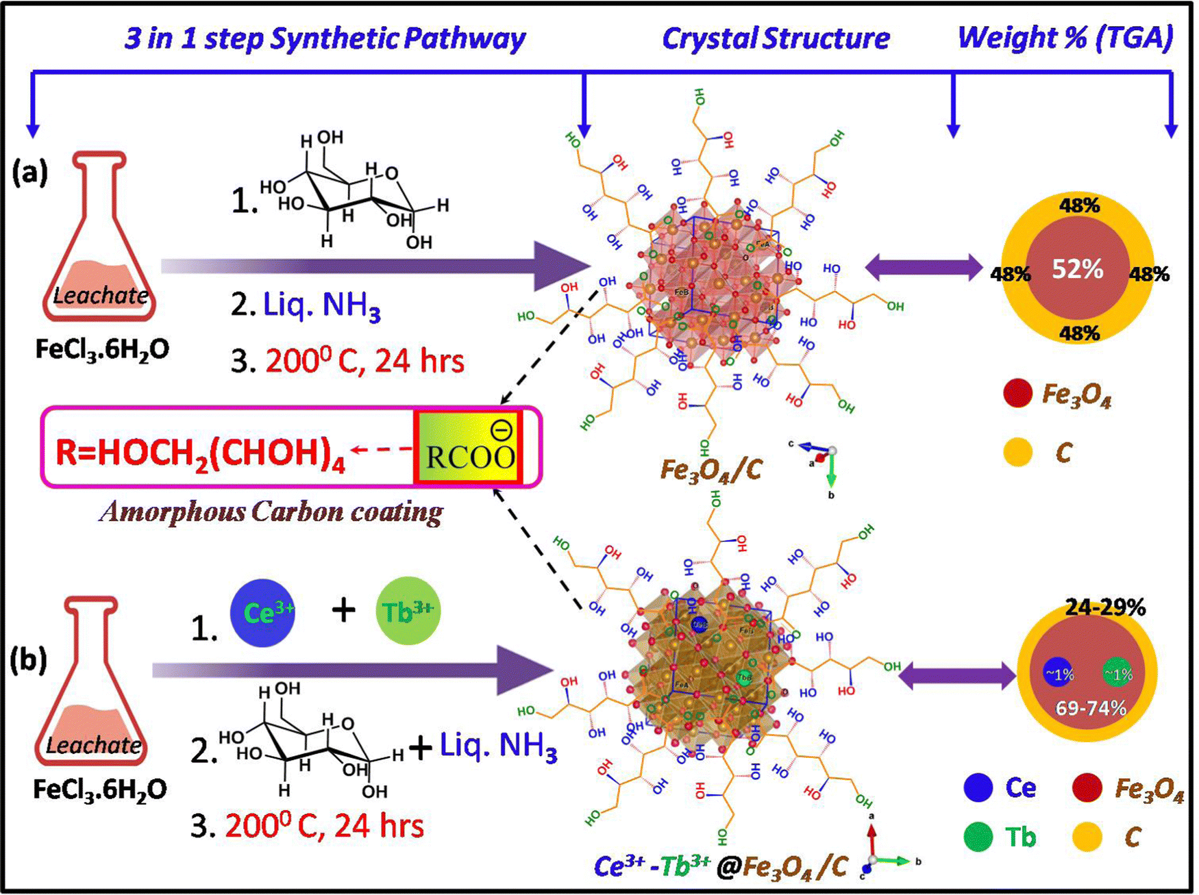 | ||
| Fig. 4 (a) Probable crystal structures (ball-stick models of the Fe3O4 lattices are created using VESTA software) and weight percentages of the core materials (in the form of circular discs) of G24. (b) Ln ion-doped G24 samples, followed by the three-step synthetic processes. | ||
4.2. TEM analysis
The morphology and microstructures of G24 and 1Ce–1Tb@G24 were determined by analyzing the TEM and HRTEM data. The TEM investigation for G24 illustrates that a huge number of Fe3O4 nanoparticles (dark gray) is consistently dispersed into the carbon sheet (light gray) (Fig. 5a).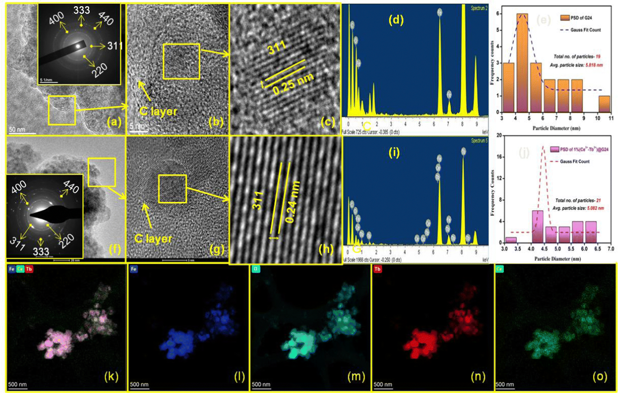 | ||
| Fig. 5 (a) TEM (50 nm); inset: SAED pattern, (b) HRTEM (5 nm), (c) lattice fringes with dhkl value, (d) EDS spectrum, (e) Particle size distribution of G24. (f) TEM (20 nm); inset: SAED pattern, (g) HRTEM (5 nm), (h) lattice fringes with dhkl value, (i) EDS spectrum, (j) particle size distribution, and (k)–(o) HAADF-STEM mapping of the Fe, O, Ce and Tb elements of 1Ce–1Tb@G24 nanoparticles, respectively. | ||
However, the particles are not identical in shape and size (polydisperse), and are enormously agglomerated in character due to their extensive superparamagnetism nature. HRTEM analysis (Fig. 5b and c) showed that the size of the smaller particles of G24 is about 10 nm. It further corroborated the presence of fringes with d-spacings (d311 = 0.25 nm) attributable to Fe3O4 throughout. The fast Fourier transform (FFT) revealed the long-range order, with SAED also displaying the crystallinity of the sample (Inset of Fig. 5a). EDX analysis (Fig. 5d) supported the view by confirming the presence of iron and oxygen in the sample. Carbon and copper signals were detected. However, these signals are likely to occur from the thin amorphous carbon membrane and the copper grid bars of the sample grid, respectively. The average nanoparticle size of G24 is 5.82 nm, as calculated from the particle distribution curve (Fig. 5e). TEM analysis for 1Ce–1Tb@G24 illustrates that a large number of Fe3O4 nanoparticles (dark gray) is homogeneously dispersed into the carbon sheet (light gray) (Fig. 5f). Fig. 5g and h show the high-magnification TEM images of that sample, where the lattice planes are visible. Here, the interplanar distance of the lattices was found to be 0.24 nm, which is equal to the value of the most intense d311 of the Fe3O4 phase. The linearity of the lattice planes signifies a lack of any planar defects and twin faults. The SAED patterns are taken from the marked regions (Inset of Fig. 5f). The spot SAED pattern implies the presence of larger particles in the marked region. All of the major diffraction spots are indexed to appear from the cubic Fe3O4. Nevertheless, the ring SAED pattern suggests the presence of smaller-sized particles in the marked region. The EDX spectrum (Fig. 5i) obtained from the doped sample confirms the presence of cerium and terbium, along with iron and oxygen. Here, the particle size distribution (calculated from the TEM images) shows that the average particle size is 5.08 nm, which is slightly smaller than that of G24 (Fig. 5j). An elemental mapping was performed using STEM-HAADF to further investigate the formation of the doped nanoparticle, shown in Fig. 5k–o. Fig. 5k shows a STEM-HAADF image of agglomerates of 1Ce–1Tb@G24. The elemental mappings are shown in Fig. 5l–o. They clearly show the well-defined spatial distributions of all of the elements present, viz., Fe, O, Tb, and Ce. The above analysis confirms the formation of the doped Fe3O4.
4.3. X-ray photoelectron spectroscopy (XPS) analysis
To estimate the elemental composition, chemical environment, and oxidation states of the different elements present in the synthesized samples, XPS spectra were acquired. The XPS survey spectra for G24 and the Ln-doped Fe3O4 are characterized in Fig. S1 (ESI†). Similar to XRD analysis, this showed no considerable signals due to impurity. The Fe 2p core level for G24 (Fig. 6a) includes the doublet, suggesting Fe 2p1/2 and Fe 2p3/2, which is allocated to the feature binding energies of magnetite (respective Fe3+ and Fe2+ ions). Furthermore, the existence of the broad Fe 2p peaks for the sample ascertains the existence of mixed iron oxide states (Fe3+ (2p3/2) and Fe2+ (2p1/2)).19 | ||
| Fig. 6 (a) Deconvoluted Fe 2p XPS spectrum for G24. (b) Deconvoluted Fe 2p XPS spectrum for 1Ce–1Tb@G24. (c) Fe 2p and (d) O 1s comparison between pure & doped G24. (e) Ce 3d and (f) Tb 4d comparison for all doped samples. Deconvoluted C 1s of (g) G24 and (h) 1Ce–1Tb@G24. | ||
Additionally, there is a slight but noticeable peak at about 718.1 eV, which is conceivably the satellite peak of Fe2+ and Fe3+ ions.46 The typical peak at about 719.0 eV for Fe3+ in the γ-Fe2O3 phase was not detected, authenticating the construction of pure Fe3O4.47Fig. 6b illustrates the deconvoluted Fe 2p core level XPS spectra for 1Ce–1Tb@G24. The Fe 2p core level XPS spectrum exhibits the peaks of Fe 2p3/2 and Fe 2p1/2 at 710.1 eV and 724.1 eV, respectively, which are ascribed to the Fe3+ state of Fe.48Fig. 6c and d demonstrate the Fe 2p and O 1s narrow-scan spectra comparison between G24 and 1Ce–1Tb@G24, respectively. Both samples consisted of two broad peaks of Fe 2p3/2 and Fe 2p1/2, which were primarily assigned to Fe–O bonds, and the values are incredibly close to those of magnetite (Fe3O4).49 A decrease in binding energy can be noticed for the Fe 2p and O 1s peaks in the doped sample compared with the equivalent peaks for pure Fe3O4. This proposes an electronic interaction between the Fe3O4 host and doped ions. The shift could be attributable to the FeIII substitution by CeIII and TbIII, which altered the FeIII:FeII ratio in samples and formed new Fe–O–Ce/Tb bonds.50 This result confirms that the lanthanide metal ion doping can slightly deform the cubic lattice structure of pure magnetite and create numerous oxygen vacancies, which are responsible for the elevation of the photocatalytic capability (see Section 4.11), as well as magnetic properties (see Section 4.10.).51 An analogous type of peak shifting was also monitored earlier for other doped samples.52,53
For all three Ln-doped samples, we have seen several medium and small peaks (Fig. 6e) between the 880 to 940 eV binding energy range. These features indicate the spin–orbit doublets, which appear because of the Ce 3d orbital spectrum on the sample surface, and prove that Ce doping occurred here with the presence of both +4 and +3 oxidation states.51 Although the peaks are not that sharp, this may be due to a low percentage of doping in the case of each doped sample.54,55
We have also confirmed the Tb doping by XPS analysis (Fig. 6f). As we can see, a sharp peak arises at ∼150 eV for each doped sample. This is mainly for the Tb 4d5/2 orbital, which supports that the doped Tb element is in the trivalent state for all Ln-doped Fe3O4/C nanospheres. However, the peak positions are slightly different for them due to different doping percentage amounts.56,57
Both the Ln-doped and undoped Fe3O4 nanospheres are highly coated with the amorphous carbon coating due to extensive D-glucose mediation at the time of hydrothermal synthesis. This fact can be proven by the C 1s peak deconvolution (Fig. 6g and h), and our group had previously reported on this phenomenon in detail.9 The HRTEM images also show the presence of an amorphous carbon coating for the samples (Fig. 5b and g). We have compared the deconvoluted C 1s peak for our best photocatalyst, i.e., 1Ce–1Tb@G24 sample, with that of G24. We see that in both cases, the carbon coating is there as a form of ferrous carboxylate and ferric carboxylate complexes, but in a different weight ratio. For both samples, the C1s raw data are deconvoluted and split into three separate sub-peaks positioned at 284.8 (sp2 C), 285.1 (sp3 C) and 287.8 (C–O bond) eV. The peak at 284.8 eV confirms the presence of D-glucose in the sample, but the other two peaks indicate that there is a partial conversion of glucose to graphitic carbon on the sample surface.58,59 For G24, we see that the peak areas of both sp3 and sp2 C (17.9% and 71.6%) are higher compared to that of 1Ce–1Tb@G24 (7.9% and 68.1%). However, its oxygen bonded C 1s peak area (10.5%) is much lower as compared to its doped analog (24.0%). This means that for doped Fe3O4, the quantity of the FeII and FeIII-carboxylate complexes is higher than that of its pure form. Hence, XPS proves that after lanthanide ion doping, the Fe3O4 nanoparticles contain more reactive oxygen species (ROS) as a carboxylate moiety and a lower quantity of carbon (as sp3 and sp2 C), which ultimately leads to a higher amount of toxic dye degradation.60 Furthermore, this result exactly matched with our FTIR and TGA analysis data in terms of how the amorphous C coating disrupts the photocatalysis rate. A greater amount of highly reactive OH˙ radicals can be generated by the iron–carboxylate complexes in both photo- and dark Fenton reactions (see Section 4.11.) in the case of the doped sample, and it finally helps to degrade the dye in a more facile way (almost 36% higher) compared to the undoped Fe3O4 nanoparticles. For better insight into the atomic composition (%) on the corresponding crystal surfaces, the XPS atomic concentration data for all samples are listed in Table S1 (ESI†).
4.4. UV-DRS analysis
UV-vis diffuse reflectance spectroscopy (DRS) was carried out to distinguish the optical properties of G24 and 1Ce–1Tb@G24. Fig. 7a depicts their reflectance spectra. The band gap energies (Eg) of the samples were calculated using the Kubelka–Munk (K–M) model.61 | ||
| Fig. 7 (a) and (b) DRS and K–M plot comparison for G24 and 1Ce–1Tb@G24. (c) FTIR absorption spectra and (d) TGA curves for all samples measured in an air atmosphere with the maximum temperature at 1000 °C and heating rate at 10 °C min−1. | ||
The following relation expresses the K–M equation at any wavelength:
 | (3) |
4.5. FTIR analysis
FTIR data afford detailed information about the molecular structure and its environment, as it is responsive to a variety of chemical bonds and functional groups present in a molecule. The corresponding spectra of all prepared samples are presented in Fig. 7c. Here, G24 exhibits64 a distinct band at 585 cm−1. This typical peak corresponds to the intrinsic stretching vibrations of metal–oxygen at the tetrahedral site.65 Most interestingly for doped samples, the band turns out to be less intense and sharper as a consequence of the interruption of the local symmetry via the introduction of Ce4+ and Tb3+ ions into the Fe3O4 host lattice. It also progressively shifted, which was attributed to the revamped bonding force between the cations and oxygen anions due to the presence of Ce3+ and Tb3+ ions.39 The band disturbances below 1500 cm−1 are attributable to the lowering of the local symmetry as a result of distortion owing to the presence of different cations at different sites.66 Additionally, the broad band between 3000 and 3600 cm−1 is recognized as the stretching vibrations of the hydroxyl groups for all samples,67 indicating the existence of water molecules adsorbed on the surface of Fe3O4, as well as the carboxylic acid or carboxylate OH groups (RCOOH = gluconic acid, acetic and formic acid), which forms during the reduction of hydrolysate (FeCl3) by D-glucose.68 Moreover, the formation of iron(II/III) carboxylate complexes is again confirmed by the medium peak at ∼1600 cm−1, indicating the presence of characteristic C![[double bond, length as m-dash]](https://www.rsc.org/images/entities/char_e001.gif) O vibrational stretching peaks, which are not available in the case of free D-glucose. Overall, the increasing carbon content on the Fe3O4 surface decreases its hydrophilic nature, and that is why G24 (having higher C wt%) is less efficient in degrading the rhodamine B dye compared to its doped analogs (having lower C wt%). In accordance with that trend, 1Ce–1Tb@G24 can degrade the highest amount of the dye because it has the lowest quantity of carbon coating.69 In this aspect, we have correlated that result with the TGA data to be discussed later (see Section 4.6).
O vibrational stretching peaks, which are not available in the case of free D-glucose. Overall, the increasing carbon content on the Fe3O4 surface decreases its hydrophilic nature, and that is why G24 (having higher C wt%) is less efficient in degrading the rhodamine B dye compared to its doped analogs (having lower C wt%). In accordance with that trend, 1Ce–1Tb@G24 can degrade the highest amount of the dye because it has the lowest quantity of carbon coating.69 In this aspect, we have correlated that result with the TGA data to be discussed later (see Section 4.6).
4.6. Thermogravimetric analysis (TGA)
Thermogravimetric analysis was performed (Temperature range = 20–950 °C) for all samples to determine the probable amount of carbon coating on each sample (Fig. 7d). Here, the thermograms can be divided into two steps of sample decomposition processes for all samples. At first, in the approximate 0–150 °C temperature range, the 1st breakdown of the material weight % occurs due to evaporation of the moisture and adsorbed water molecules on their surfaces.70,71 For G24, the majority of H2O molecules are dissociated (∼11% of the total weight of the sample) compared to the doped G24 samples. This phenomenon can be well explained by BET analysis (see Section 4.9.).In terms of the 2nd step of the weight % dissociation in the ∼250–950 °C T region, the reason may be mainly thermal disintegration of different inorganic and organic functional groups, as well as the hydroxyl group, which can undergo complexation with the central host metal ions, i.e., Fe3+/Fe2+ of the magnetite nanoparticles.72 In this case, G24 clearly gives the maximum loss of weight (∼48%) to others, which confirms the highest amount of carbon coating in G24. With an increase in doping amount, the coating becomes lower and reaches the minimum value for our best catalyst, i.e., 1Ce–1Tb@G24. The circular discs for the weight % values of the sub-components of the G24 and Ln-doped G24 samples are given in Fig. 4, where the amount of ‘C’ coating on the catalyst's surface follows the following descending order, i.e., G24 > 0.5Ce-1Tb@G24 > 1Ce–0.5Tb@G24 > 1Ce–1Tb@G24.
It should also be noted that the trend for catalytic efficiency towards dye degradation is exactly the opposite. From these two reciprocal relations, we can conclude that the carbon coating hinders the induction of direct light on the reactive surfaces of the photocatalysts. Furthermore, it further delays or suppresses the electron–hole generation from its valence bands (VB). This phenomenon has been already reported in our previous work.9 However, after ∼500 °C, all of the samples show a stable magnetite (Fe3O4) structure, as no further decay of thermograms occurred after that crucial temperature, and then the curve becomes saturated. Moreover, the lanthanide ion doping may decrease the carbon coating percentage on the catalytic surface according to their low weight loss values in the 2nd thermal dissociation step.73,74 Overall, we can say that all of the doped and undoped Fe3O4 nanoparticles may be coated with different amounts of carbon plausibly due to the formation of Fe2+-(RCOO)n2−n and Fe3+-(RCOO)n3−n complexes through glucose mediation.35
4.7. Mott–Schottky analysis
To visualize the type of semiconducting property and the probable band energy levels, an electrochemical Mott–Schottky experiment was done. The fundamentals of this test involve the dependence of the electrochemical impedance on the experimental potential range, which can be converted to the capacitance.75,76 The capacitance and the potential are related by the following equation:| 1/C2 = (2/A2eεε0ND) (E − EFBP − kT/e) | (4) |
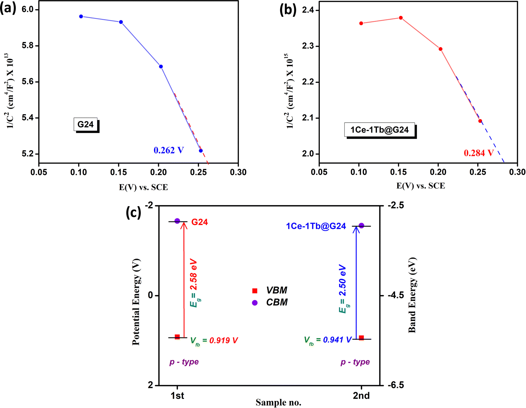 | ||
| Fig. 8 Mott–Schottky diagrams for (a) G24 and (b) 1Ce–1Tb@G24. (c) Comparison plot of the respective band positions for G24 and 1Ce–1Tb@G24. | ||
Therefore, by convention, the EFBP values for both materials symbolize the valence band maxima (VBM), and the photo-induced charge carriers residing at VBM are the holes (h+). It should be noted that the EFBP value of the undoped material is 0.262 V, while the doped material shows a greater +ve EFBP value (0.284 V). The potential against SCE is converted to the ERHE through the following equation:
| ERHE = ESCE + 0.059 pH + E°SCE | (5) |
| SI No. | Sample name | Optical band gap (eV) | FB potential (for VBM) (V vs. RHE) | Charge carrier density |
|---|---|---|---|---|
| 1 | G24 | 2.58 | 0.919 | 5.79 × 10¹⁴ |
| 2 | 1-1Ln@G24 | 2.50 | 0.941 | 1.55 × 10¹⁶ |
This result authenticates that on illumination, the doped material can create higher h+ density at the VBM, which can considerably produce extremely reactive. OH˙ radicals in solution for the outstanding photocatalytic oxidation reaction. Additionally, the overall picture of the possible band energy diagram recommends that the introduction of the lanthanide ions help in tunneling the photo-induced e− from Fe3O4 CBM into the lanthanide interface to diminish the charge pair recombination, and consequently catalyze the reaction through greater h+ density at the VBM of the hybrid semiconductor materials.
4.8. Photoluminescence data
 | ||
| Fig. 9 (a) Fluorescence decay spectra comparison; inset: colorimetric image of the UV ray irradiated sample dispersed in ethanol. (b) Plausible energy level diagram of 1Ce–1Tb@G24, where the red, blue, and green arrows signify the radiative decays for the Ce3+ and Tb3+ ions, respectively, and a big white dotted arrow represents the non-radiative decay process from the 5d orbital of Ce3+ to that of Tb3+ ion. (c) CIE chromaticity diagram of 1Ce–1Tb@G24 showing its chromatic coordinate (x,y). (d) Time-resolved decay curves of G24 and Ln-doped G24 samples. | ||
The PL spectra of G24 are found to be broad and asymmetric. The emission band at about 497 nm may be ascribed to surface defects of the Fe3O4 lattice.77,78 However, some new peaks in the range of 400–460 nm with a large hump (∼490 nm) appeared in the case of doped samples compared to G24. Among the Ln-doped G24 samples, only 1Ce–1Tb@G24 shows a highly intense cyan color under a UV lamp (365 nm light source). Previous reports show that for Ce3+ ion-doped compounds, a fluorescence emission normally appears in the 410–460 nm region, which produces a violet-blue colorband.79,80 Here, the three medium peaks at 403, 429, and 454 nm are prominent in the case of 1Ce–1Tb@G24 compared to other samples, which show a cyan color under UV light irradiation. The Tb-containing metal oxide nanoparticles mainly give a green fluorescence (520–570 nm range), as reported previously.81,82 However, no prominent peaks for Tb3+ are observed herein for co-doping. After doping, no major sharp peaks for both Ln3+ ions can be identified for all doped samples, which may be attributed to the presence of a very low percentage of doping, where the sharp Ln3+-associated peaks are submerged inside the broad peak of pure Fe3O4. Nevertheless, the resultant strong cyan color for 1Ce–1Tb@G24 may appear due to the unequal mixing of two basic colors, i.e., blue and green. The supported plausible energy diagram (Fig. 9b) shows how the excited electrons sensitize the excited electronic states of Tb3+ ions via a non-radiative pathway. Also, a CIE diagram is given (Fig. 9c) to evaluate the expected color co-ordinate, i.e., (0.2,0.2), for the cyan emission of the sample, which is the main cause for co-doping instead of single doping inside the G24 lattice.83
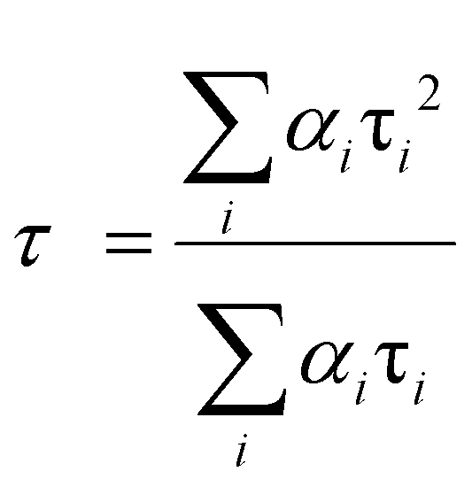 | (6) |
All of the decay curves are fitted with a tri-exponential.84,85 The decay components (τ1, τ2, τ3), amplitude of the components (b1, b2, b3), and the average decay time 〈τ〉 for different samples are summarized in Table 4.
| SI No. | Sample's name | Relative amplitudes [B] (%) | Lifetimes [τi2] (ns) | χ 2 value | Average lifetime (ns) | Decay constant [K] (ns−1) | ||||
|---|---|---|---|---|---|---|---|---|---|---|
| B 1 | B 2 | B 3 | T 1 | T 2 | T 3 | |||||
| 1 | 1Ce–1Tb@G24 | 46.44 | 10.14 | 43.42 | 2.60 | 0.595 | 8.38 | 1.09 | 6.86 ± 0.34 | 0.14 ± 0.01 |
| 2 | 1Ce–0.5Tb@G24 | 45.68 | 44.31 | 10.02 | 2.71 | 8.06 | 0.561 | 1.07 | 6.61 ± 0.33 | 0.15 ± 0.01 |
| 3 | 0.5Ce-1Tb@G24 | 47.61 | 11.30 | 41.09 | 2.59 | 0.478 | 7.93 | 1.02 | 6.39 ± 0.32 | 0.16 ± 0.01 |
| 4 | G24 | 45.99 | 10.72 | 43.29 | 2.48 | 0.447 | 7.59 | 1.01 | 6.21 ± 0.31 | 0.16 ± 0.01 |
The fast decay component is due to the radiative recombination process of electrons and holes at luminescent sites, and the slow decay component typically appears from the defect-related emission.86 Generally, doped nanomaterials are expected to have longer exciton decay times due to the spatial separation of charges.87 Herein, the average decay time value for 1Ce–1Tb@G24 is found to be higher than those of G24 due to the trap emission of the Fe3O4 nanoparticles.83
An analysis reveals that the relaxation dynamics are influenced by defect states, which are formed by the dopant ions. Thus, Ce,Tb-codoped Fe3O4 samples are expected to have a longer exciton decay time due to the spatial separation of the charges. Furthermore, the higher value of the average decay time (6.86 ns) indicates the effective charge separation in the doped sample, which leads to improved photocatalytic activity. These results are also consistent with the FTIR and XRD studies.
4.9. BET surface area analysis
For heterogeneous photocatalysis, the surface area plays a fundamental role.88 Herein, the BET surface areas and pore size distributions of each sample were determined by measuring nitrogen adsorption–desorption isotherms (Fig. 10a). | ||
| Fig. 10 (a) N2 adsorption–desorption isotherms. (b) BJH Pore size distribution. (c) Linear BET surface area plot comparison of G24 and 1Ce–1Tb@G24. | ||
Both the adsorption and desorption branches of each isotherm produced a particular H2 type hysteresis loop attributed to type IV behavior.89 This indicates the presence of interconnected mesoporous networks with disordered and inhomogeneous size distributions, resulting from the aggregation of the primary nanocrystallites (Fig. 10b). The linear BET plot comparison (Fig. 10c) shows different slopes and intercepts, indicating different surface areas for doped and G24. The specific BET surface areas were found to be 59.639 and 15.849 m2g−1 for G24 and 1Ce–1Tb@G24, respectively (Table 5).
| SI No. | Sample name | Multipoint BET surface area (m2 g−1) | Total pore volume (cc g−1) | BET constant (c) | BJH pore radius (Å) |
|---|---|---|---|---|---|
| 1 | G24 | 59.639 | 0.0548 | 31.257 | 17.757 |
| 2 | 1Ce–1Tb@G24 | 15.849 | 0.1901 | 35.523 | 6.822 |
It is important to note that although the particle sizes of both samples are roughly comparable, it is expected that their surface area will be very close. However, consistent with some previous relevant research works, we have found that the as-synthesized Ln-doped G24 samples are more agglomerated in nature, which may cause a certain decrease of their surface area compared to that of pure G24.90,91 Notably, the surface area of G24 exceeds that of 1Ce–1Tb@G24, which argued against a simple correlation between the surface area and photocatalytic activity. It should also be noted that the porosity of the material is considerably lower for 1Ce–1Tb@G24 compared to G24 (Table 5). This result indicates that for G24, the adsorption phenomenon dominates compared to the light-utilizing effect in terms of dye removal. However, adsorption is not a useful technique in terms of complete dye fragmentation. It is also very tough to reproduce the catalyst for further use due to the almost permanent occupancy of the dye molecules on the catalytic active sites.9 However, despite having a lower surface area, due to the higher utilization of light energy, the doped sample shows superior dye degradation efficiency, as well as better catalytic reproducibility.
4.10. Static magnetic properties
In Fig. 11a, we have an analogous S-shaped hysteresis loop for the M vs. H plot for all of the samples.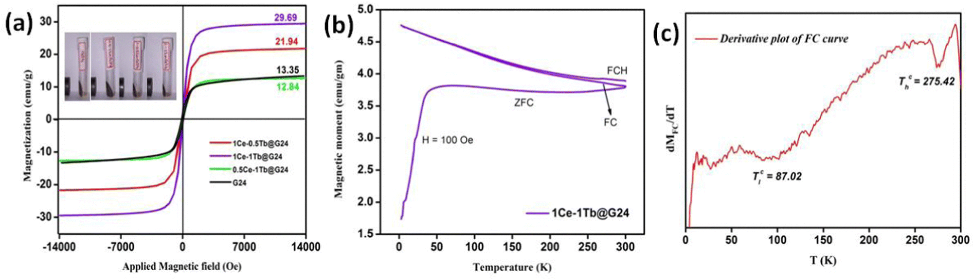 | ||
| Fig. 11 (a) Magnetic moment vs Applied field curves of pure and doped G24 samples. (b) FC-ZFC-FCH curve and (c) Transition temperature derivation plot of 1Ce–1Tb@G24. | ||
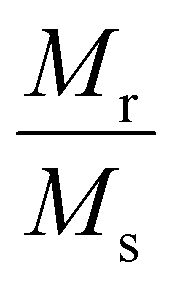
Concerning the bulk Fe3O4 material (∼92 emu g−1), for all doped and undoped G24, we have observed lower magnetic saturation values due to the presence of the ‘Carbon’ coating on the particle surface. Also, the grain size of the nanoparticles has hardly any effect on the variation of the Ms values, as there is no significant alteration of the particle sizes observed in all of the samples (see Section 4.1). Besides that, as a result of the low coercivity (Hc) and very low squareness ratio (Mr/Ms), all of the samples can be termed as superparamagnetic9 (Table 6).
| Sample | Average crystallite size (D) (nm) XRD | M s (emu g−1) | M r (emu g−1) | Squareness ratio
|
H c(Oe) |
|
|---|---|---|---|---|---|---|
| G-24 | 27.96 | 13.35 | 2.265 | 0.169 | 73.09 | 1016.40 |
| 0.5Ce-1Tb@G24 | 25.78 | 12.84 | 1.367 | 0.106 | 83.47 | 1116.41 |
| 1Ce–0.5Tb@G24 | 24.92 | 21.94 | 2.075 | 0.094 | 99.81 | 2281.07 |
| 1Ce–1Tb@G24 | 26.28 | 29.69 | 3.308 | 0.111 | 68.78 | 2127.16 |
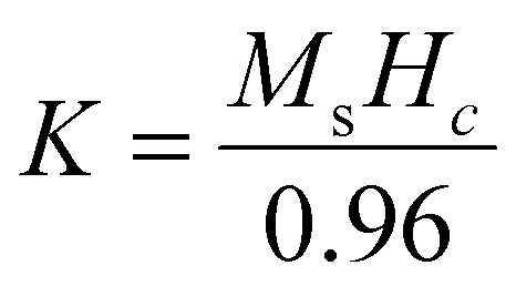
For the Ln-doped Fe3O4 nanocrystals, the rare earth metal ions (here, Ce3+ and Tb3+) substitute the Fe3+ ions in the octahedral B site of the Fe3O4 crystal lattices and the Ms value eventually increases due to A–B super exchange interaction.92 Furthermore, for the anisotropic constant (K), the trend is also identical, i.e., the K value increases with increasing doping percentage due to the advanced spin–orbit coupling effect.93 This phenomenon is due to the deformation of the pure Fe3O4 crystal symmetry via lattice strain through lanthanide ion doping.94
Magnetization vs. temperature data were measured at 100 Oe magnetic field and a temperature range from 2 K to 300 K (Fig. 11b). The field cooling (FC – 2 K to 300 K), zero field cooling (ZFC – 300 K to 2 K) and field cooled heating (FCH – 2 K to 300 K) can all be observed in that plot. The 1st derivative (Fig. 11c) of the FC curve provides two transition temperatures for 1Ce–1Tb@G24, which has the highest magnetic saturation value among all of the samples. At ∼87 °C, the 1st transition temperature (Tc) may appear owing to the ferro- to antiferromagnetic transition. Meanwhile, the 2nd Tc can be observed at ∼275 °C, i.e., at a higher temperature region, and this may be due to the para- to ferromagnetic transition of the material.95,96
4.11. Photocatalytic activity and mechanism
In order to investigate the photocatalytic activity of the as-prepared G24 and Ce,Tb-codoped G24 samples, several experiments were conducted under different reaction conditions. For each experiment, 25 mg of each catalyst was used along with 50 mL of 1.0 × 10⁻⁵ M aqueous solution of RhB (pH 7), and the absorption band of RhB was witnessed at about 555 nm (λmax). Fig. 12a illustrates the relationship between the light absorbance and simulated solar irradiation time for all of the samples mentioned above, and Fig. 12b shows the bar diagram representation of the RhB removal percentage against the doping weight percent ratio in G24. | ||
| Fig. 12 (a) Sample variation in the RhB photocatalysis absorbance plots under visible light excitation by using 25 mg catalyst and H2O2 within 180 min. (b) Bar diagram representation of the dye removal % with the variation of the Ln doping ratio in G24. | ||
It was observed that the absorption band steadily decreased for all of the samples with increasing light irradiation time. However, the degradation is characteristically higher (97.0 (± 0.7)%) for the 1Ce–1Tb@G24 sample. Fig. 13a–d illustrate the relationships between the light absorbance and simulated solar irradiation time (t) for G24 and the corresponding three different ratios-variated Ln-doped G24 samples with H2O2.
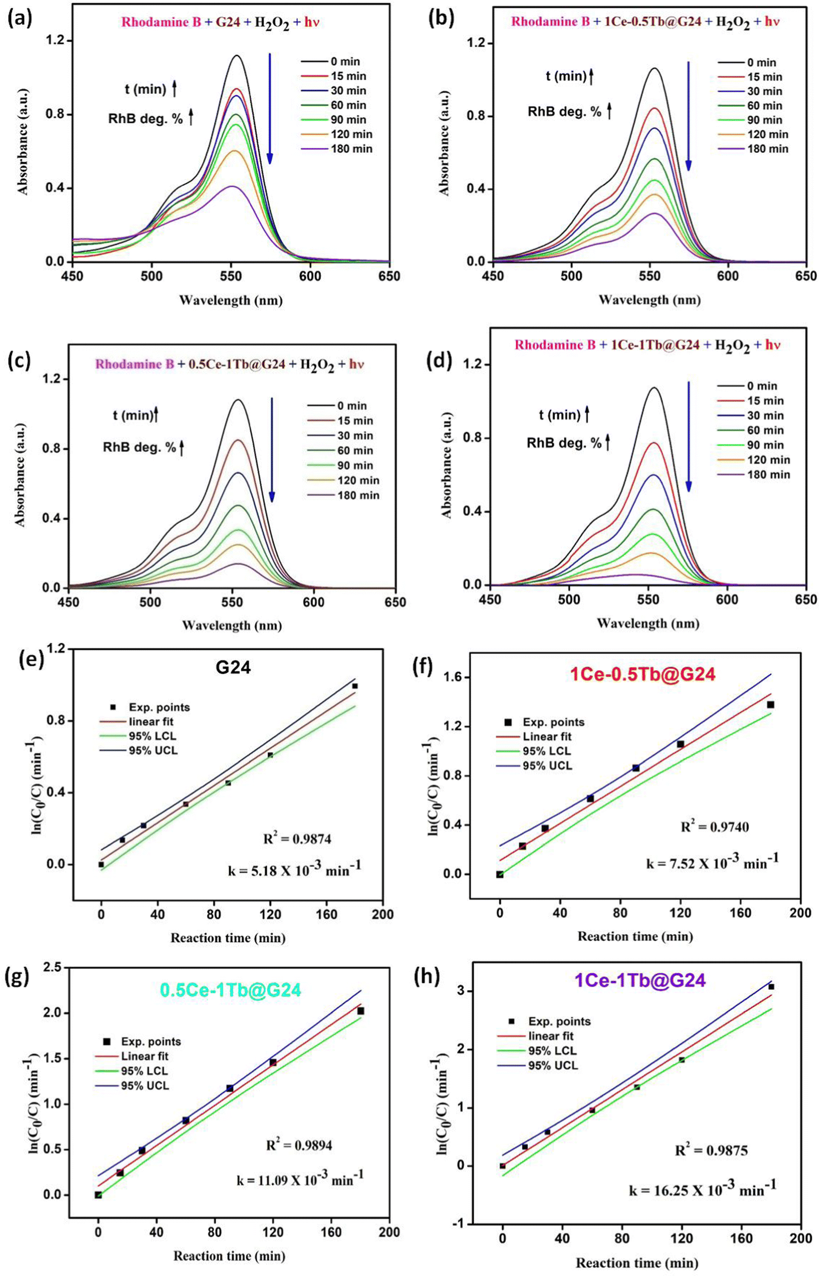 | ||
| Fig. 13 (a)–(d) Absorbance curves for the photocatalytic treatment of 50 mL 10−5 M RhB aqueous solutions (λmax = 555 nm) by using G24 and other Ln-doped G24 samples (25.0 mg) with the addition of 100 μL H2O2 as an initiator in each case. (e-h) Rate constant derivation plots as ln(C0/C) vs. illumination time (t = 0–180 min) in the presence of corresponding samples under visible light excitation with 100 μL H2O2. | ||
It was witnessed that in all of the cases, the absorption band gradually decreased with increasing irradiation time (t), although the rate of decrease was highest in the case of 1Ce–1Tb@G24 among all of the samples. It was observed that the discoloration of RhB in the presence of a doped sample is considerably higher than that in the presence of the pure sample. To quantitatively evaluate the photocatalytic activities of these samples, the reaction rate constants (k) were calculated by adopting the pseudo-first-order kinetics model, assuming low initial pollutant concentration.97
| ln(C0/C) = kt | (7) |
Plots of ln(C0/C) vs. irradiation time (t) are provided in Fig. 13e–h. The linear relationships pointing to each photodegradation follow first-order kinetics. The apparent rate constants were estimated to be 5.18 × 10⁻³ and 16.25 × 10⁻³ min−1 for G24 and 1Ce–1Tb@G24, respectively, which signifies that the photocatalytic activity of the best catalyst is about 3 times higher than that of the pure sample.
It is essential to investigate the stability of the photocatalytic performance and the reusability of the best photocatalyst reported here (1Ce–1Tb@G24). Also, this is an important factor from economic and environmental perspectives.98 To investigate the stability and reusability of that photocatalyst, cycling experiments for the photodegradation of RhB were conducted with the catalyst. After each recyclability test, the catalyst was recovered from the solution using an external magnetic field, washed with water and absolute ethanol, dried at 80 °C for 2–3 h, and then used for the following cycles. As shown in Fig. 14a, the degradation efficiencies of 1Ce–1Tb@G24 over RhB after the first, second, and third cycles were found to be ∼ 95, 94, and 91%, respectively.
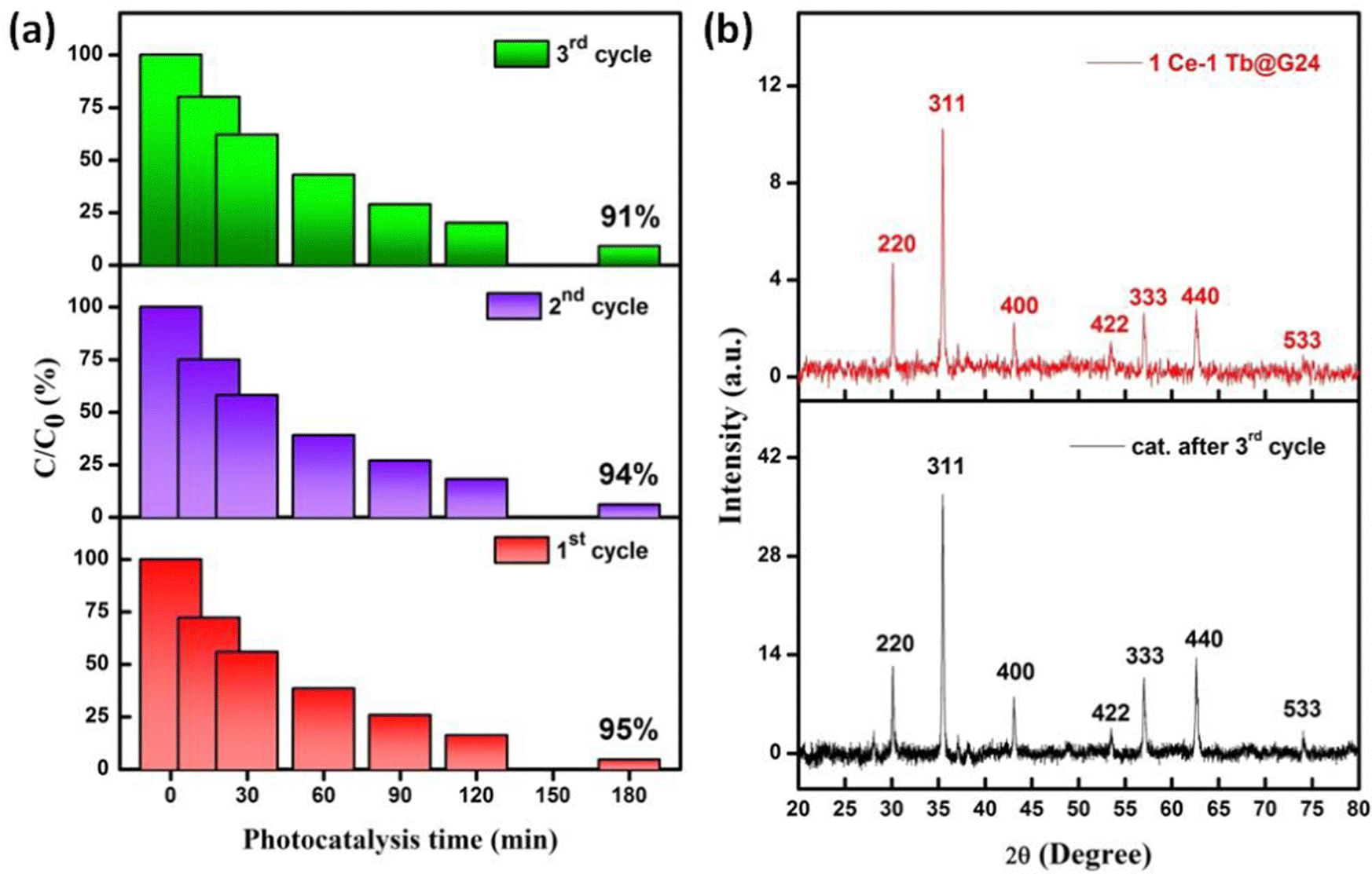 | ||
| Fig. 14 (a) Recyclability test (as shown by the stacked bar diagrams) of 1Ce–1Tb@G24 up to the 3rd cycle as the C/C0 (%) vs. t plot, where C0 and C are the initial concentration and concentrations at time t (after irradiation of the dye), respectively. (b) Pre- and post-catalytic (3rd cycle) XRD differentiation data of 1Ce–1Tb@G24. | ||
In addition, it is noted that about 2.7, 1.09, and 0.487% of the initial quantity of the catalyst was lost in each cycle. Overall, these data suggest that a slight reduction in the photocatalytic efficiency could be attributed to the inevitable loss of the catalyst during the recovery steps.99 We also consider that the reduced effectiveness of the catalyst after recycling is due to the photobleaching of the catalyst surface.89,100
Furthermore, Fig. 14b displays the XRD patterns of 1Ce–1Tb@G24 before and after three RhB decomposition cycles, with the lack of noticeable changes signifying that both the crystalline phase and structure remain intact. Also, we have compared the FTIR data between the pre- and post-catalytic sample (Fig. S2, ESI†), which again confirm the fact that the photocatalyst remains almost structurally unchanged. So, from both XRD and FTIR analysis, we can conclude that even after 3 photoreduction cycles, the catalyst can be reused multiple times with a small amount of degradation % loss.
Photocatalytic properties of semiconductors depend on the capability to produce electron–hole pairs and the construction of free radicals for secondary reactions.88 Here, we have made a plausible mechanism of RhB dye photocatalysis by G24 and Ln-doped G24 samples under simulated solar irradiation specified by the chain of the following SET (single electron transfer) reactions [eqn (8)–(21)]:
In the valence band (VB) of G24 or Ln-doped G24 samples,
| Fe3O4 (hVB+) + H2O → Fe3O4 + ˙OH | (8) |
In the conduction band (CB) of G24 or Ln-doped G24 samples,
| Fe3O4 (1eCB−) + H2O2 → ˙OH + OH− + Fe3O4 | (9) |
| Fe3O4 (1eCB−) + O2 → Fe3O4 + ˙O2− | (10) |
| ˙O2− + H2O2 → ˙OH+ OH− + O2 | (11) |
| ˙O2− + H2O → HO2˙+ OH− | (12) |
| Fe3+-(RCOO)n3−n + Fe3O4(1eCB−) → Fe2+-(RCOO)n2−n | (13) |
| Fe2+-(RCOO)n2−n → Fe3+-(RCOO)n3−n + 2e− | (14) |
| 2e− + H2O2 → ˙OH + OH− | (15) |
| Fe3+-(RCOO)n3−n + H2O2 → Fe2+-(RCOO)n2−n + HO2˙ + H+ | (16) |
| Fe3+-(RCOO)n3−n + H2O + hν (light source) → Fe2+-(RCOO)n2−n + OH + H+ | (17) |
In the CB of only Ln-doped G24 samples, some extra SET reactions occur:
| Ln4+ + Fe3O4 (1eCB−) → Ln3+˙[Ln = Ce, Tb] | (18) |
| Ln3+ → Ln4+ + 3e− [Ln = Ce, Tb] | (19) |
| 3e− + H2O2 → ˙OH + OH− | (20) |
Final photocatalytic pathway:
| ˙OH/˙O2− + RhB → CO2 + H2O | (21) |
{Note: the left superscripts of the free electrons in the equations denote the electrons used in or generated from different types of reactions}.
We know that bulk Fe3O4 normally can show either n- or p-type behavior,9 unlike the case of other simple n-type101 or p-type102 semiconductor systems. Herein, from the Mott–Schottky analysis, we have proved that both the doped and undoped materials show only a p-type semiconducting nature, which can be related to the effective charge carrier separation for conducting the photocatalysis process. During the excitation of light, an electron (e−) in the VB of the semiconductor is excited to the CB with the concurrent generation of a hole (h+) in the VB of G24 or Ln-doped G24. In the VB state, the holes are neutralized by some adsorbed water molecules to form extremely reactive hydroxyl radicals (˙OH) [eqn (8)]. Then, the excited electrons in the CB can be trapped by the initiator H2O2 and free O2 to form highly reactive •OH and deprotonated superoxide radical anions (˙O2−), respectively [eqn (9) and (10)]. These radicals can enormously increase their numbers via some chain reactions with initiator H2O2 and water [eqn (11) and (12)]. However, from the eqn (10)–(12), it becomes clear that among all of the reactive oxygen species, the ˙OH is the primary reactive species here.
From the radical scavenger experiment, the presence of hydroxyl radicals is further confirmed through the fluorescence on–off test for terephthalic acid (TA).9 TA is a non-fluorescent compound. However, in the presence of reactive ˙OH radicals, it converts to 2-hydroxy terephthalic acid (2HTA), which can show very high fluorescence. So, with increasing time in the photocatalytic process, more ˙OH is produced in the reaction media and ultimately reacts with TA to increase the fluorescence color intensity. For G24, the corresponding peak intensity increases very slowly (Fig. 15a). For 1Ce–1Tb@G24, the rate of fluorescence intensity increment becomes very high (Fig. 15b). This occurs since the number of •OH increases considerably for the Ln-doped G24 catalysts owing to a lesser amount of electron–hole recombination. This result establishes that after doping, G24 turns out to be more efficient towards the photocatalytic removal of RhB dye.
 | ||
| Fig. 15 Radical scavenging test using the fluorescence spectral measurement of TA for (a) G24 and (b) 1Ce–1Tb@G24. | ||
From eqn (11), we can see that the amount of ˙O2− becomes negligible through the reaction with H2O2 to form more ˙OH radicals. The HO2˙ radicals are less reactive compared to ˙OH radicals due to their lower oxidation potential9 (eqn (12)). Furthermore, eqn (13)–(15) illustrate how the amorphous C coating (as a form of FeII/FeIII-gluconate component) intrinsically takes part in the free electrons generation, which lastly reacts with initiator H2O2 and can form more ˙OH species. However, for both G24 and 1Ce–1Tb@G24, the abovementioned eqn (14) and (15) belong to the Fenton reaction, and eqn (14) gives the dark Fenton reaction. Eqn (17) here corroborates well with the the photo-Fenton mechanisms, which have been broadly explained in our previous work.9 Here, both iron–carboxylate complexes act as a photo-Fenton reagent, which can produce hydroxyl radicals without the help of the initiator.103
Consistent with the abovementioned equations, we have prepared a feasible catalytic reaction scheme for both G24 and 1Ce–1Tb@G24 (Fig. 16).
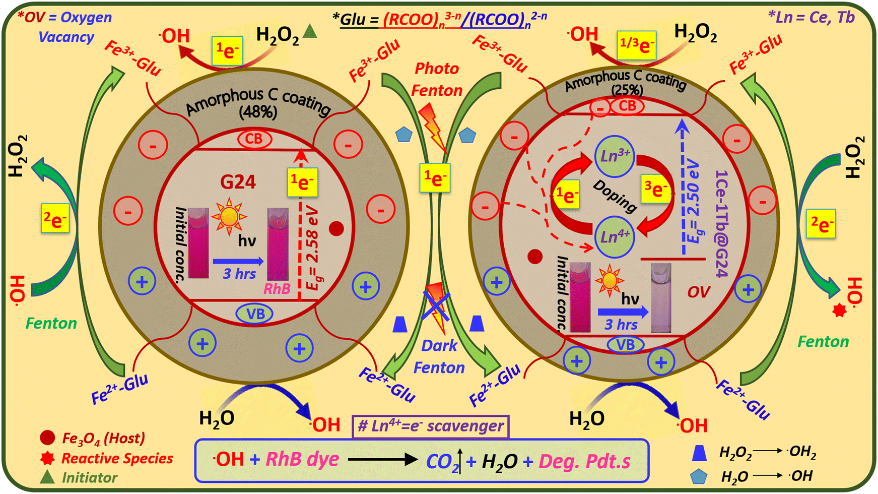 | ||
| Fig. 16 Plausible single electron transfer pathway of the photocatalytic RhB degradation mechanism for both G24 and 1Ce–1Tb@G24 samples. Inset: Corresponding colorimetric images of aqueous solutions of RhB for the initial data before and after degradation using G24 and 1Ce–1Tb@G24 samples are given. The excited free electrons are marked by numbers from 1 to 3 (as the left superscripts of their corresponding single electron symbols), indicating different types of Single Electron Transfer (SET) pathways. | ||
Recently, it has been found that suitable metal ion-doped Fe3O4 may increase the photocatalytic efficiency by increasing the charge separation, which is akin to some other core–shell type materials.104,105 Here, two aspects essentially control the photocatalysis rate: one is the surface area, and another is the excited e− tunneling through the trapped states of the dopant ions. With a much larger specific surface area, nanoparticles possess stronger adsorption ability and increased available active surface sites.102 As G24 has a higher surface area compared to 1Ce–1Tb@G24, the chances of dye adsorption are higher in G24 rather than its fragmentation via photocatalysis. The effect of surface area on the photocatalytic efficiency has already been discussed in detail in Section 4.9. Additionally, from the Mott–Schottky analysis (Section 4.7.), we have proved that for Ln-doped G24 samples, the photoinduced electrons are easily captured by the doping-related trapped states compared to the undoped G24. Accordingly, the recombination of photoinduced electron–hole pairs is efficiently inhibited and the photocatalytic efficiency is considerably promoted.106 A few scientists also proved that rare earth ion doping can enhance the photocatalytic efficiency.51,107 Again, from the XPS study of the Ln-doped G24 samples, it is already confirmed that both Ln+4 and Ln3+ ions are present inside the Fe3O4 lattice (see Section 4.3.). The oxygen vacancies generated inside the Ln-doped G24 lattice created by Ln4+/3+ ions lead to a decrease in the electron–hole recombination process. Here, Ln4+ can act as an e− scavenger, which attracts excited electrons from both the conduction band of Fe3O4 and the amorphous C coating around the sample, and considerably prevents the recombination of +ve and –ve charges51 (Fig. 16). As a result, an effective cyclic e− transfer occurs from Ce3+/Tb3+ to Ce4+/Tb4+ and vice versa [eqn (18) and (19)] in the Ln-doped G24, which are responsible for the greater •OH generation from H2O2 compared to that of G24 [eqn (20)]. At last, the ˙OH radicals and the holes left in the valence band can react with the adsorbed pollutant molecules (RhB dye) to produce several oxidized species and/or decomposed products,108 which eventually leads to CO2 and water [eqn (21)].
Moreover, we have also prepared two similar types of lanthanide ion-doped G24 samples; one by using pure FeCl3 (laboratory grade) and the other by using IOTs. We have elaborately compared the physical and photochemical properties of the IOTs-derived 1Ce–1Tb@G24 and FeCl3-derived 1Ce–1Tb@G24. It is observed that both samples show identical properties. The details of this comparison study are given in the ESI† (Section 1.3, Fig. S3–S5, ESI†). From the results, we can conclude that it is unnecessary to synthesize 1Ce–1Tb@G24 through a conventional and more expensive approach (by using lab chemical FeCl3). Rather, it can be prepared by a more environmentally benign and cost-effective approach from toxic and value-less IOTs (mining wastes).
Therefore, from the above results it can be concluded that the photocatalytic activity of the as-prepared samples is outstanding in terms of rhodamine B dye degradation, which is found to be superior compared to a few formerly reported active photocatalysts (Table 7).109–118
| SI No. | Catalyst name | Reaction time (h & min) | Reaction temperature (°C) | Nature of light source | pH of reaction medium | Catalyst amount (mg) or conc. (g L−1 or ppm) | Dye initial Conc. (gm L−1 or ppm) | Removal efficiency (mg g−1 or %) | Magnetically recoverable (Yes/No) | Ref. |
|---|---|---|---|---|---|---|---|---|---|---|
| a r.t. – Room temperature. b NF – Not found. | ||||||||||
| 1 | MIL53Fe@MIL53Sr | 1 | NF | 300 W Xenon-lamp (Both Visible & UV) | NF | 2.5 g L−1 | 0.02 g L−1 | 67 | No | 109 |
| 2 | ZnO/Bi2MoO6 | 4 | NF | 15 W visible light lamp | 7.54 | 0.25 g L−1 | 10 ppm | 92 | No | 110 |
| 3 | DA-CTF | 1 | NF | Visible light (380–750 nm, 7 W) | NF | 0.2 g L−1 | 0.03 g L−1 | 92.3 | No | 111 |
| 4 | Ag@ZnO | 3 | r.t. | 60 W Hg lamp | 2–12 | 0.2–0.5 g L−1 | 10 ppm | 91 | No | 112 |
| 5 | monoBODIPY-functionalized Fe3O4@SiO2@TiO2 | 1 | 25 °C | UV lamp | NF | 1 g L−1 | 30 ppm | 29.49 | Yes | 113 |
| 6 | Fe3O4@TiO2/Ag,Cu | 1 h, 30 min | r.t. | 500 W Hg Lamp | NF | 5 ppm | NF | 86.19 | Yes | 114 |
| 7 | 0.5%Zn-doped Fe3O4 | 5 | r.t. | UV lamp | NF | 30 mg | 0.01 g L−1 | 97 | Yes | 115 |
| 8 | Fe3O4/TiO2 nanocomposites | 2 | r.t. | 300 W Xenon lamp | 3–9 | 20–60 mg | 0.005–0.025 g L−1 | 91 | Yes | 116 |
| 9 | 3% Ta@TiO2 | 2 | r.t. | 125 W, UV 365 nm lamp | NF | 30 mg | 10 ppm | 92 | No | 117 |
| 10 | PPy/SnO2 | 1 h, 30 min | NF | LED 8 W | NF | 10 mg | 0.1 ppm | 63.6 | No | 118 |
| 11 | (Ce3+ + Tb3+) ion-doped and carbon-coated Fe3O4 | 3 | r.t. (30 °C) | LED Xenon lamp (100 W) | 7 | 25 mg | 10 ppm | ∼98 | Yes | Our work |
5. Conclusions
In brief, we have effectively fabricated fluorescent-supermagnetic-photocatalytic Ce,Tb-codoped Fe3O4 nanocrystals by a straightforward, low-cost, and environmentally benign hydrothermal reduction route from a low-cost iron precursor acquired from accumulated iron ore tailings (IOTs). This innovative method eliminates both the price of adding lab-based Fe precursors and the high temperatures and complexity of prior single salt processes. The structural analysis established the occurrence of a single phase with an inverse spinal structure at all doping levels. Various techniques have been exploited to characterize these trifunctional nanocrystals, and the outcomes illustrate their bright fluorescence and strong magnetism. Associated with outstanding optical and magnetic properties, the economically prepared Ce,Tb-codoped Fe3O4 nanocrystals reveal tremendous photocatalytic activity in the treatment of toxic dye. The UV-DRS analysis, TCSPC measurement, and Mott–Schottky analyses authenticate the necessity, as well as the usefulness of lanthanide ion doping in pure Fe3O4 crystal. The dye removal efficiency was found to be ∼98% and the efficiency was maintained roughly at the same scale even after 3 cycles. Hence, the results confirm the validity of the as-synthesized nanomaterials in environmental applications such as the removal of toxic pollutants from the environment. Furthermore, the presence of a considerable amount of organic carbon coating may act as a main electron supplier in the photocatalytic reaction, which can be appropriate for use in environmental and biomedical applications. The method we used here can be straightforwardly extended to the synthesis of other nanomaterials based on lanthanide-doped materials and metal oxides for various wastewater treatment applications.Author contributions
Utsav Sengupta: creation of the concept, methodology, data accretion, original manuscript preparation, and its proper analysis. Muthaimanoj Periyasamy: resources and visualization. Sudipta Mukhopadhyay: resources and validation. Arik Kar: supervision, conceptualization, reviewing, and editing draft.Conflicts of interest
The authors declare no competing financial interest.Acknowledgements
A. K. acknowledges support from the Department of Science and Technology (DST), Government of India through its INSPIRE Faculty Award Programme (Award No. DST/INSPIRE/04/2016/000790). A. K. also acknowledges support from the Royal Society's Newton International Fellowship Follow-on Funding Scheme (Award No. AL/201058). The DST INSPIRE fellowship division, India financially supported the PhD of U.S. We are very much thankful to the ACMS, IIT Kanpur for providing the BET and XPS data and S. N. Bose National Centre for Basic Sciences, Kolkata for the powder XRD and TGA-DTA data. IACS Kolkata provided us with the MPMS data for magnetic analysis. The elemental mapping (using STEM-HAADF) for all samples was performed by the Department of Chemistry, University of Cambridge. Besides this, we want to convey special thanks to Dr Jit Satra, IOP Bhubaneswar for giving us some valuable suggestions for conducting the Mott–Schottky experiment and Dr Pradipta Purakayastha, IISER Kolkata for helping with the TCSPC measurement. TEM measurements with SAED images were given by SAIF, IIT Bombay. We are also very thankful for FTIR, which was done by the Materials Science and Engineering Department, IIEST Shibpur. Lastly, we want to convey a special thanks to the ‘BioRender.com’ website for helping us to create the synthetic method flow chart diagram.References
- H. Lee, A. M. Purdon, V. Chu and R. M. Westervelt, Nano Lett., 2004, 4, 995–998 CrossRef CAS.
- J. Xie, K. Chen, H. Y. Lee, C. Xu, A. R. Hsu, S. Peng, X. Chen and S. Sun, J. Am. Chem. Soc., 2008, 130, 7542–7543 CrossRef CAS PubMed.
- X. Wang, Y. Du, S. Ding, Q. Wang, G. Xiong, M. Xie, X. Shen and D. Pang, J. Phys. Chem. B, 2006, 110, 1566–1570 CrossRef CAS PubMed.
- S. Y. Yu, H. J. Zhang, J. B. Yu, C. Wang, L. N. Sun and W. D. Shi, Langmuir, 2007, 23, 7836–7840 CrossRef CAS PubMed.
- S. A. Corr, Y. P. Rakovich and Y. K. Gunko, Nanoscale Res. Lett., 2008, 3 Search PubMed.
- C. Plank, Trends Biotechnol., 2008, 26, 59–63 CrossRef CAS PubMed.
- Z. F. Li and E. Ruckenstein, Nano Lett., 2004, 4, 1463–1467 CrossRef CAS.
- X. Yu, L. Chen, Y. Deng, K. Li, Q. Wang, Y. Li, S. Xiao, L. Zhou, X. Luo, J. Liu and D. Pang, J. Fluores., 2007, 17, 243–247 CrossRef CAS PubMed.
- M. Periyasamy, S. Sain, M. Mandal, U. Sengupta, S. Mukhopadhyay and A. Kar, Mater. Adv., 2021, 2, 4843–4858 RSC.
- J. Kim, J. E. Lee, J. Lee, J. H. Yu, B. C. Kim, K. An, Y. Hwang, C. H. Shin, J. G. Park, J. Kim and T. Hyeon, J. Am. Chem. Soc., 2005, 128, 688–689 CrossRef PubMed.
- G. Lv, F. He, X. Wang, F. Gao, G. Zhang, T. Wang, H. Jiang, C. Wu, D. Guo, X. Li, B. Chen and Z. Gu, Langmuir, 2008, 24, 2151–2156 CrossRef CAS PubMed.
- C. Boxall, G. Kelsall and Z. Zhang, J. Chem. Soc., Faraday Trans., 1996, 92, 791–802 RSC.
- L. Tan and T. R. Allen, Corros. Sci., 2009, 51, 2503–2507 CrossRef CAS.
- P. Mishra, S. Patnaik and K. Parida, Catal. Sci. Technol., 2019, 9, 916–941 RSC.
- Z. Zhu, Z. Lu, D. Wang, X. Tang, Y. Yan, W. Shi, Y. Wang, N. Gao, X. Yao and H. Dong, Appl. Catal., B, 2016, 182, 115–122 CrossRef CAS.
- R. Hassandoost, S. R. Pouran, A. Khataee, Y. Orooji and S. W. Joo, J. Hazard. Mater., 2019, 376, 200–211 CrossRef CAS PubMed.
- S. Gao, C. Guo, J. Lv, Q. Wang, Y. Zhang, S. Hou, J. Gao and J. Xu, Chem. Eng. J., 2017, 307, 1055–1065 CrossRef CAS.
- S. Chidambaram, B. Pari, N. Kasi and S. Muthusamy, J. Alloys Compd., 2016, 665, 404–410 CrossRef CAS.
- L. Geng, B. Zheng, X. Wang, W. Zhang, S. Wu, M. Jia, W. Yan and G. Liu, ChemCatChem, 2016, 8, 805–811 CrossRef CAS.
- H. Jin, X. Tian, Y. Nie, Z. Zhou, C. Yang, Y. Li and L. Lu, Environ. Sci. Technol., 2017, 51, 12699–12706 CrossRef CAS PubMed.
- S. R. Pouran, A. Bayrami, A. A. Aziz, W. M. A. W. Daud and M. S. Shafeeyan, J. Mol. Liq., 2016, 222, 1076–1084 CrossRef.
- G. S. Parkinson, Z. K. Novotny, P. Jacobson, M. Schmid and U. Diebold, J. Am. Chem. Soc., 2011, 133, 12650–12655 CrossRef CAS PubMed.
- H. Yao and Y. Ishikawa, J. Phys. Chem. C, 2015, 119, 13224–13230 CrossRef CAS.
- X. Wu, J. Tang, Y. Zhang and H. Wang, Mater. Sci. Eng. B, 2009, 157, 81–86 CrossRef CAS.
- X. Sun, C. Zheng, F. Zhang, Y. Yang, G. Wu, A. Yu and N. Guan, J. Phys. Chem. C, 2009, 113, 16002–16008 CrossRef CAS.
- L. Hadian-Dehkordi and H. Hosseini-Monfared, Green Chem., 2016, 18, 497–507 RSC.
- E. V. Groman, J. C. Bouchard, C. P. Reinhardt and D. E. Vaccaro, Bioconjugate Chem., 2007, 18, 1763–1771 CrossRef CAS PubMed.
- X. Wang and Y. Li, Chem. – Eur. J., 2003, 9, 5627–5635 CrossRef CAS PubMed.
- F. Wang, Y. Zhang, X. Fan and M. Wang, J. Mater. Chem., 2006, 16, 1031 RSC.
- X. F. Yu, L. D. Chen, M. Li, M. Y. Xie, L. Zhou, Y. Li and Q. Q. Wang, Adv. Mater., 2008, 20, 4118–4123 CrossRef CAS.
- P. Drake, H.-J. Cho, P.-S. Shih, C.-H. Kao, K.-F. Lee, C.-H. Kuo, X.-Z. Lin and Y.-J. Lin, J. Mater. Chem., 2007, 17, 4914 RSC.
- X. Liang, X. Wang, J. Zhuang, Y. Chen, D. Wang and Y. Li, Adv. Funct. Mater., 2006, 16, 1805–1813 CrossRef CAS.
- M. F. Casula, Y.-W. Jun, D. J. Zaziski, E. M. Chan, A. Corrias and A. P. Alivisatos, J. Am. Chem. Soc., 2006, 128, 1675–1682 CrossRef CAS PubMed.
- V. O. Almeida and I. A. H. Schneider, Miner. Eng., 2020, 156, 106511 CrossRef CAS.
- M. Periyasamy, S. Sain, E. Ghosh, K. J. Jenkinson, A. E. Wheatley, S. Mukhopadhyay and A. Kar, Environ. Sci. Pollut. Res., 2021, 29, 6698–6709 CrossRef PubMed.
- Y. Sun, X. Zhang, Y. Han and Y. Li, Powder Technol., 2020, 361, 571–580 CrossRef CAS.
- Z. He, Y. Xia, J. Su and B. Tang, Opt. Mater., 2019, 88, 195–203 CrossRef CAS.
- Z. He, H. Yang, J. Su, Y. Xia, X. Fu, L. Wang and L. Kang, Fuel, 2021, 294, 120399 CrossRef CAS.
- A. Aashima, S. Uppal, A. Arora, S. Gautam, S. Singh, R. J. Choudhary and S. K. Mehta, RSC Adv., 2019, 9, 23129–23141 RSC.
- B. P. Ladgaonkar and A. S. Vaingankar, Mater. Chem. Phys., 1998, 56, 280–283 CrossRef CAS.
- D. Padalia, U. C. Johri and M. G. H. Zaidi, Mater. Chem. Phys., 2016, 169, 89–95 CrossRef CAS.
- S. Nagashima, K. Ueda and T. Omata, J. Phys. Chem. C, 2022, 126, 6499–6504 CrossRef CAS.
- A. Aguirre Giraldo, I. Moncayo-Riascos and R. Ribadeneira, Energy Fuels, 2022, 36, 5228–5239 CrossRef CAS.
- E. Hannachi, Y. Slimani, M. Nawaz, Z. Trabelsi, G. Yasin, M. Bilal, M. A. Almessiere, A. Baykal, A. Thakur and P. Thakur, J. Phys. Chem. Solids, 2022, 170, 110910 CrossRef CAS.
- E. Rai, R. S. Yadav, D. Kumar, A. K. Singh, V. J. Fulari and S. B. Rai, J. Lumin., 2022, 241, 118519 CrossRef CAS.
- S. Sathish and S. Balakumar, Mater. Chem. Phys., 2016, 173, 364–371 CrossRef CAS.
- J. A. Cuenca, K. Bugler, S. Taylor, D. Morgan, P. Williams, J. Bauer and A. Porch, J. Phys.: Condens. Matter, 2016, 28, 106002 CrossRef PubMed.
- M. Muhler, R. Schlogl and G. Ertl, J. Catal., 1992, 138, 413–444 CrossRef CAS.
- J. Lu, X. L. Jiao, D. R. Chen and W. Li, J. Phys. Chem. C, 2009, 113, 4012–4017 CrossRef CAS.
- Z. Qi, T. P. Joshi, R. Liu, H. Liu and J. Qu, J. Hazard. Mater., 2017, 329, 193–204 CrossRef CAS PubMed.
- S. J. Singh and P. Chinnamuthu, Colloids Surf., A, 2021, 625, 126864 CrossRef CAS.
- S. Liu, E. Guo and L. Yin, J. Mater. Chem., 2012, 22, 5031–5041 RSC.
- Y. Xiong, C. Tang, X. Yao, L. Zhang, L. Li, X. Wang, Y. Deng, F. Gao and L. Dong, Appl. Catal., A, 2015, 495, 206–216 CrossRef CAS.
- B. Janani, M. K. Okla, B. Brindha, T. M. Dawoud, I. A. Alaraidh, W. Soufan, M. A. Abdel-Maksoud, M. Aufy, C. R. Studenik and S. S. Khan, New J. Chem., 2022, 46, 16844–16857 RSC.
- Y. Li, L. Wu, Y. Wang, P. Ke, J. Xu and B. Guan, J. Water Process Eng., 2020, 36, 101313 CrossRef.
- Y. Zhang, G. K. Das, R. Xu and T. T. Yang Tan, J. Mater. Chem., 2009, 19, 3696 RSC.
- P. Gong, Q. Chen, K. Shih, C. Liao, L. Wang, H. Xie and S. Deng, J. Mater. Sci.: Mater. Electron., 2019, 30, 20970–20978 CrossRef CAS.
- T. Wu, Y. Liu, X. Zeng, T. Cui, Y. Zhao, Y. Li and G. Tong, ACS Appl. Mater. Interfaces, 2016, 8, 7370–7380 CrossRef CAS PubMed.
- Y. Liu, Y. Li, K. Jiang, G. Tong, T. Lv and W. Wu, J. Mater. Chem. C, 2016, 4, 7316–7323 RSC.
- Z. Luo, J. Wang, Y. Song, X. Zheng, L. Qu, Z. Wu and X. Wu, ACS Sustainable Chem. Eng., 2018, 6, 13262–13275 CrossRef CAS.
- P. Kubelka and F. Munk, Z. Tech. Phys., 1931, 12, 259–274 Search PubMed.
- A. Kar and A. Patra, J. Phys. Chem. C, 2009, 113, 4375–4380 CrossRef CAS.
- A. Kar, S. Kundu and A. Patra, RSC Adv., 2012, 2, 10222–10230 RSC.
- W. B. White and B. A. D. Anoelis, Spectrochim. Acta, Part A, 1967, 23, 985–995 CrossRef CAS.
- M. Abboud, S. Youssef, J. Podlecki, R. Habchi, G. Germanos and A. Foucaran, Mater. Sci. Semicond. Process., 2015, 39, 641–648 CrossRef CAS.
- J. Tang, M. Myers, K. A. Bosnick and L. E. Brus, J. Phys. Chem. B, 2003, 107, 7501–7506 CrossRef CAS.
- M. Y. Nassar and M. Khatab, RSC Adv., 2016, 6, 79688–79705 RSC.
- H. Zhang, N. Li, X. Pan, S. Wu and J. Xie, Green Chem., 2016, 18, 2308–2312 RSC.
- J. Yang, J.-Y. Li, J.-Q. Qiao, S.-H. Cui, H.-Z. Lian and H.-Y. Chen, Appl. Surf. Sci., 2014, 321, 126–135 CrossRef CAS.
- A. Demir, R. Topkaya and A. Baykal, Polyhedron, 2013, 65, 282–287 CrossRef CAS.
- Z. Razmara, S. Saheli, V. Eigner and M. Dusek, Appl. Organomet. Chem., 2019, 33, e4880 CrossRef.
- A. Ansari, N. Ahmad, M. Alam, S. F. Adil, S. M. Ramay, A. Albadri, A. Ahmad, A. M. Al-Enizi, B. F. Alrayes, M. E. Assal and A. A. Alwarthan, Sci. Rep., 2019, 9, 7747 CrossRef PubMed.
- M. N. Luwang, S. Chandra, D. Bahadur and S. K. Srivastava, J. Mater. Chem., 2012, 22, 3395 RSC.
- M. Osial, P. Rybicka, M. Pękała, G. Cichowicz, M. Cyrański and P. Krysiński, Nanomaterials, 2018, 8, 430 CrossRef PubMed.
- J. Satra, P. Mondal, U. K. Ghorui and B. Adhikary, Sol. Energy Mater. Sol. Cells, 2019, 195, 24–33 CrossRef CAS.
- J. Satra, P. Mondal, G. R. Bhadu and B. Adhikary, Mater. Adv., 2023, 4, 2340–2353 RSC.
- M. Sadat, M. Kaveh Baghbador, A. W. Dunn, H. Wagner, R. C. Ewing, J. Zhang, H. Xu, G. M. Pauletti, D. B. Mast and D. Shi, Appl. Phys. Lett., 2014, 105, 091903 CrossRef.
- D. Shi, M. Sadat, A. W. Dunn and D. B. Mast, Nanoscale, 2015, 7, 8209–8232 RSC.
- X. He, X. Liu, R. Li, B. Yang, K. Yu, M. Zeng and R. Yu, Sci. Rep., 2016, 6, 22238 CrossRef CAS PubMed.
- S. Hur, H. J. Song, H.-S. Roh, D.-W. Kim and K. S. Hong, Ceram. Int., 2013, 39, 9791–9795 CrossRef CAS.
- Y. Wang, S. Zhong, X. Wen and Q. Zhang, Inorg. Chem. Commun., 2022, 135, 109099 CrossRef CAS.
- X. Sang, J. Lian, N. Wu, X. Zhang and J. He, Polyhedron, 2019, 169, 114–122 CrossRef CAS.
- L. U. Khan, G. H. da Silva, A. M. de Medeiros, Z. U. Khan, M. Gidlund, H. F. Brito, O. Moscoso-Londoño, D. Muraca, M. Knobel, C. A. Pérez and D. S. Martinez, ACS Appl. Nano Mater., 2019, 2, 3414–3425 CrossRef CAS.
- S. Mondal, S. Sudhu, S. Bhattacharya and S. K. Saha, J. Phys. Chem. C, 2015, 119, 27749–27758 CrossRef CAS.
- R. Sinha, A. Chatterjee and P. Purkayastha, J. Phys. Chem. B, 2022, 126, 1232–1241 CrossRef CAS PubMed.
- A. Kar, S. Kundu and A. Patra, J. Phys. Chem. C, 2011, 115, 118–124 CrossRef CAS.
- A. Kar and A. Patra, Trans. Ind. Ceram. Soc., 2013, 72, 89–99 CrossRef CAS.
- A. Kar, S. Sain, S. Kundu, A. Bhattacharyya, S. Kumar Pradhan and A. Patra, Chem. Phys. Chem., 2015, 16, 1017–1025 CrossRef CAS PubMed.
- A. Kar, S. Sain, D. Rossouw, B. R. Knappett, S. K. Pradhan and A. E. Wheatley, Nanoscale, 2016, 8, 2727–2739 RSC.
- B. Boruah, R. Gupta, J. M. Modak and G. Madras, Nanoscale Adv., 2019, 1, 2748–2760 RSC.
- A. H. Asif, N. Rafique, R. A. Hirani, H. Wu, L. Shi and H. Sun, J. Colloid Interface Sci., 2021, 604, 390–401 CrossRef CAS PubMed.
- K. P. Hazarika and J. P. Borah, J. Magn. Magn. Mater., 2022, 560, 169597 CrossRef CAS.
- C. R. De Silva, S. Smith, I. Shim, J. Pyun, T. Gutu, J. Jiao and Z. Zheng, J. Am. Chem. Soc., 2009, 131, 6336–6337 CrossRef CAS PubMed.
- F. J. Douglas, D. A. MacLaren, N. Maclean, I. Andreu, F. J. Kettles, F. Tuna, C. C. Berry, M. Castro and M. Murrie, RSC Adv., 2016, 6, 74500–74505 RSC.
- R. Singh, S. Kumar Srivastava, A. K. Nigam, V. V. Khovaylo, L. K. Varga and R. Chatterjee, J. Appl. Phys., 2013, 114, 243911 CrossRef.
- P. Granitzer, K. Rumpf, M. Venkatesan, A. G. Roca, L. Cabrera, M. P. Morales, P. Poelt and M. Albu, J. Electrochem. Soc., 2010, 157, K145 CrossRef CAS.
- S.-R. I. Sloman, S. Sain, J. Olszówka, S. K. Pradhan, A. E. H. Wheatley and A. Kar, Mater. Chem. Phys., 2022, 277, 125463 CrossRef CAS.
- A. Kar, S. Sain, D. Rossouw, B. R. Knappett, S. K. Pradhan, G. A. Botton and A. E. H. Wheatley, J. Alloys Compd., 2017, 698, 944–956 CrossRef CAS.
- A. Kar, J. Olszówka, S. Sain, S.-R. I. Sloman, O. Montes, A. Fernández, S. K. Pradhan and A. E. H. Wheatley, J. Alloys Compd., 2019, 810, 151718 CrossRef CAS.
- Y. Yang, D. S. Kim, Y. Qin, A. Berger, R. Scholz, H. Kim, M. Knez and U. Gosele, J. Am. Chem. Soc., 2009, 131, 13920–13921 CrossRef CAS PubMed.
- M. Periyasamy, A. Saha, S. Sain, M. Mandal, U. Sengupta and A. Kar, J. Environ. Chem. Eng., 2020, 8, 104604 CrossRef CAS.
- U. Sengupta, A. Mukherjee, M. Periyasamy, S. Mukhopadhyay, K. J. Jenkinson, A. E. Wheatley and A. Kar, New J. Chem., 2023, 47, 11425–11443 RSC.
- T. Han, L. Qu, Z. Luo, X. Wu and D. Zhang, New J. Chem., 2014, 38, 942–948 RSC.
- Z. He, M. Siddique, H. Yang, Y. Xia, J. Su, B. Tang, L. Wang, L. Kang and Z. Huang, J. Cleaner Prod., 2022, 339, 130634 CrossRef CAS.
- Z. He, H. Yang, N. H. Wong, L. Ernawati, J. Sunarso, Z. Huang, Y. Xia, Y. Wang, J. Su, X. Fu and M. Wu, Small, 2023, 19, 2207370 CrossRef CAS PubMed.
- Z. He, H. Fareed, H. Yang, Y. Xia, J. Su, L. Wang, L. Kang, M. Wu and Z. Huang, J. Colloid Interface Sci., 2023, 629, 355–367 CrossRef CAS PubMed.
- A. Popa, M. Stefan, D. Toloman, O. Pana, A. Mesaros, C. Leostean, S. Macavei, O. Marincas, R. Suciu and L. Barbu-Tudoran, Powder Technol., 2018, 325, 441–451 CrossRef CAS.
- Y. Nosaka, S. Komori, K. Yawata, T. Hirakawa and A. Y. Nosaka, Phys. Chem. Chem. Phys., 2003, 5, 4731–4735 RSC.
- M. Humayun, M. He, W. Feng, C. Jin, Z. Yao, Y. Wang, W. Pi, S. Ali, A. Khan, M. Wang, Z. Zheng, Q. Fu, H. Xia and W. Luo, Sol. Energy, 2021, 215, 121–130 CrossRef CAS.
- T. Chankhanittha and S. Nanan, J. Colloid Interface Sci., 2021, 582, 412–427 CrossRef CAS PubMed.
- Y. Zhuang, Q. Zhu, G. Li, Z. Wang, P. Zhan, C. Ren, Z. Si, S. Li, D. Cai and P. Qin, Mater. Res. Bull., 2022, 146, 111619 CrossRef CAS.
- M. Ahmad, M. T. Qureshi, W. Rehman, N. H. Alotaibi, A. Gul, R. S. Abdel Hameed, M. A. Elaimi, M. F. H. Abdel-kader, M. Nawaz and R. Ullah, J. Alloys Compd., 2022, 895, 162636 CrossRef CAS.
- A. Bilgic, J. Alloys Compd., 2022, 899, 163360 CrossRef CAS.
- H. Ghafuri, M. Dehghani, A. Rashidizadeh and M. Rabbani, Optik, 2019, 179, 646–653 CrossRef CAS.
- A. Manohar, K. Chintagumpala and K. H. Kim, J. Mater. Sci.: Mater. Electron., 2021, 32, 8778–8787 CrossRef CAS.
- N. Madima, K. K. Kefeni, S. B. Mishra, A. K. Mishra and A. T. Kuvarega, Inorg. Chem. Commun., 2022, 145, 109966 CrossRef CAS.
- R. Paul, K. Kavinarmatha and S. Parthiban, J. Mol. Struct., 2023, 1277, 134869 CrossRef CAS.
- S. Sagadevan, J. Anita Lett, G. K. Weldegebrieal, S. Imteyaz and M. R. Johan, Chem. Phys. Lett., 2021, 783, 139051 CrossRef CAS.
Footnote |
| † Electronic supplementary information (ESI) available. See DOI: https://doi.org/10.1039/d3ma00689a |
| This journal is © The Royal Society of Chemistry 2023 |