Rapid quantitative analysis of rare earth elements Lu and Y in rare earth ores by laser induced breakdown spectroscopy combined with iPLS-VIP and partial least squares

Abstract

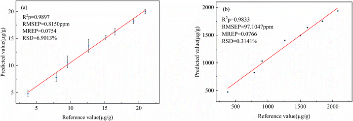
Rare earth ores are complex in composition and diverse in mineral composition, requiring high technical requirements for the selection of rare earth ores. It is of great significance to explore the on-site rapid detection and analysis methods of rare earth elements in rare earth ores. Laser induced breakdown spectroscopy (LIBS) is an important tool to detect rare earth ores, which can be used for in situ analyses without complicated sample preparation. In this study, a rapid quantitative analysis method for rare earth elements Lu and Y in rare earth ores was established by LIBS combined with an iPLS-VIP hybrid variable selection strategy and partial least squares (PLS) method. First, the LIBS spectra of 25 samples were studied using laser induced breakdown spectrometry. Second, taking the spectrum processed by wavelet transform (WT) as the input variables, PLS calibration models based on interval partial least squares (iPLS), variable importance projection (VIP) and iPLS-VIP hybrid variable selection were constructed to quantitatively analyze rare earth elements Lu and Y, respectively. The results show that the WT-iPLS-VIP-PLS calibration model has better prediction performance for rare earth elements Lu and Y, and the optimal coefficient of determination (R²) of Lu and Y were 0.9897 and 0.9833, the root mean square error (RMSE) were 0.8150 μg g⁻¹ and 97.1047 μg g⁻¹, and the mean relative error (MRE) were 0.0754 and 0.0766, respectively. It shows that LIBS technology combined with the iPLS-VIP and PLS calibration model provides a new method for in situ quantitative analysis of rare earth elements in rare earth ores.

---

1. Introduction

The composition of rare earth minerals is complex and diverse, and the exploration process of rare earth minerals needs to be completed through a combination of multiple processes, which requires higher technical requirements. Rare earth ores are the main raw material for obtaining rare earths. It is the general name of seventeen metal elements of the lanthanide series in the periodic table of rare earth elements and scandium and yttrium. Rare earths have unique atomic structure, excellent photo-electromagnetic properties and can easily be combined with other elements, which can be widely used in metallurgy,¹ petrochemical,² medicine,^3,4 computer manufacturing,⁵ agriculture and other fields. With the development of emerging industries, rare earths are becoming more and more important in national security and sustainable economic development. The addition of rare earth metals to steel can play a role in refining, desulfurization, neutralization of low melting point harmful impurities, and it can improve the processing properties of steel.⁶ Lutetium can be made into some special alloys, and its aluminum alloy can be used for neutron activation analysis. The stable lutetium nuclide can play a catalytic role in petroleum cracking, alkylation, hydrogenation and polymerization. Yttrium can be used as an additive for steel and nonferrous metal alloys. Adding a small amount of yttrium to magnesium alloys can improve the corrosion resistance of the alloys.⁷ The stable yttrium zirconia solid will be used as electrolyte of fuel cell. Yttrium is used for controlling rods of nuclear reactors, etc. Rare earth has become a necessary raw material for the development of sophisticated industries around the world. The extensive application of rare earths has led to an increasing global demand.⁸ It is of great significance to explore a method that can quickly detect and analyse rare earths in situ for the exploration of rare earths.

The common used analytical methods for rare earth elements are neutron activation analysis (NAA),⁹ inductively coupled plasma emission spectrometry (ICP-OES),¹⁰ inductively coupled plasma mass spectrometry (ICP-MS)^11,12 and X-ray fluorescence spectrometry (XRF),¹³ etc. However, the above methods have more or less disadvantages. For example, when ICP-OES, ICP-MS and NAA technologies are used to detect rare earths in rare earth ores, complex pretreatment is required, which is very time-consuming and cannot be used for real-time online detection and on-site analysis. XRF technologies have many influencing factors such as the low content of rare earth elements and serious overlap of spectral lines. Therefore, there is an urgent need for a rapid and accurate in situ detection and analysis method of rare earth elements. Laser-induced breakdown spectroscopy (LIBS), as a novel and promising analytical technique, shows several obvious advantages, such as rapid, real-time, in situ, micro-destructive analysis, remote detection and simultaneous multielement analysis. It has been widely used in space exploration,¹⁴ geological exploration,^15,16 medical diagnosis,^17,18 metallurgical analysis,¹⁹ food detection,^20,21 chemical industry²² and other fields. At present, the LIBS technique has become an international research focus for geological exploration including rock analysis,²³ identification of ore grade.²⁴ Akhmetzhanov et al.²⁵ used LIBS technology to detect rare-earth elements – Ce, La, Nd, Pr and Sm – in ores, and the results show that LIBS have potential to quantify rare earth elements in natural ores. Martin et al.²⁶ used LIBS analyses rare earth elements Eu, Gd, La, Nd, Pr and Sm, and the calibration R² for each element were ranging from 0.95 to 0.99. Bhatt et al.²⁷ used LIBS analyses of six rare earth elements Ce, Eu, Gd, Nd, Sm and Y, and the limits of detection for Ce, Eu, Gd, Nd, Sm and Y were calculated to be 0.098%, 0.052%, 0.077%, 0.047%, 0.250%, and 0.036%, respectively. Therefore, the application of LIBS technology in the analysis of rare earth ores is feasible.

The LIBS information is very complex because of the complex matrix of rare earth ore, which reduces the accuracy of LIBS technology in the analysis of rare earths. Chemometrics analysis methods, such as partial least squares (PLS),²⁸ random forest (RF),^29–31 artificial neural networks (ANN),³² support vector machine (SVM),³³ and other algorithms, provide effective tools for accurate quantitative analysis of LIBS technology. PLS is one of the most commonly used modeling methods in chemometrics. It uses rich spectral information to compensate for different deviations, making the quantitative model more stable. Guan et al.³⁴ predicted the carbon content of pulverized coal by LIBS combined with PLS. The prediction error is about 0.41%, and R² is about 0.991. The LIBS spectrum usually includes a large number of high-dimensional data, which affects the prediction accuracy of multivariate calibration. Feature selection, as an important preprocessing step in data mining, can eliminate redundant variables, reduce data dimensions and select effective variables to improve the performance of multivariate calibration models.³⁵ In order to improve the accuracy of LIBS analysis, the hybrid variable selection method is adopted. Hybrid variable selection³⁶ is a combination of wave bands and wave points methods. It first uses the wave bands method to “rough selection” and the relevant intervals were selected. And then passes the remaining features along with the concentration data as input parameters to the wave points method for “fine selection”, and the relevant variable points were selected. Hybrid method usually achieves high accuracy that is characteristic to wave bands and high efficiency characteristic to wave points.

Therefore, this study attempted to use LIBS combined with iPLS-VIP and PLS for rapid and accurate quantitative analysis of Lu and Y in rare earth ores. The rare earth ore samples were collected by LIBS spectrograph and the initial PLS calibration model was established. Additionally, the effects of different pretreatment methods and variable selection on the PLS model are explored. We believe that the results of this study will allow cheaper, sensitive, accurate, and direct determination of Lu and Y in ore analysis using LIBS, which provides a feasible method for on-site quantitative analysis of rare earth elements in ores.

2. Material and methods

2.1 Sample preparation

In this experiment, four kinds of rare earth ore standard sample powders (GBW07158, GBW07159, GBW07160 and GBW07161 rare earth ore standard samples purchased from Nanjing Zhongbiao Chenxi Chemical Technology Co., Ltd, China) were mixed in different proportions to prepare 25 samples of rare earth ores. A certain amount of standard material was removed before using, dried at 105 °C for one hour, and cooled to indoor temperature in a desiccator. Weigh different proportions of standard sample powders, and grind them in a mortar for 5 to 10 minutes, so that the sample powders can be mixed evenly. Table 1 lists the reference values (in wt%) of some elements in 25 samples of rare earth ore. The content of rare earth element Lu ranges from 2 to 30 μg g⁻¹, the content of element Y ranges from 180 to 3030 μg g⁻¹, and the content of some other macronutrients ranges from 260 to 745 500 μg g⁻¹. The content of rare earth elements in rare earth ores are less compared to the macronutrients, and element Y is the most abundant element in rare earth ore. In order to avoid scattering of the sample due to the high pulsed laser energy, polyvinyl alcohol was used as a binder when pressing the pellets to improve the tightness of the pressed pellets. Weighing 0.5000 g of the mixed rare earth ore sample powder and 0.8000 g of polyvinyl alcohol, a PC-24 tablet press (Pinchuang Technology, pressure: 30 MPa) was used to maintain the press for 5 minutes to produce a Φ20 mm × 4 mm pressed pellets, one pressed tablet for each of the 25 rare earth ore samples, for a total of 25 pressed pellets.

Table 1 Reference values (in wt%) of some elements in 25 samples of rare earth ores

Sample no.	Reference values (10^−2)				Reference values (10^−6)
	Si	Ca	Fe	Mg	Lu	Y
#1	67.28	0.033	3.561	0.229	2.0	180.0
#2	74.55	0.026	1.204	0.077	5.5	570.0
#3	74.34	0.031	1.169	0.080	30.4	3030.0
#4	66.72	0.029	3.532	0.231	13.6	1240.0
#5	70.92	0.030	2.383	0.153	3.8	380.0
#6	70.81	0.032	2.365	0.155	16.2	1610.0
#7	67.00	0.031	3.547	0.230	7.8	710.0
#8	74.45	0.029	1.187	0.079	18.0	1800.0
#9	70.64	0.028	2.368	0.154	9.6	910.0
#10	70.53	0.030	2.351	0.156	22.0	2140.0
#11	72.06	0.030	1.978	0.129	12.6	1260.0
#12	69.52	0.029	2.766	0.179	7.0	660.0
#13	69.45	0.031	2.754	0.180	15.3	1480.0
#14	71.87	0.029	1.968	0.129	16.5	1610.0
#15	70.72	0.030	2.367	0.154	12.9	1260.0
#16	72.13	0.028	1.990	0.128	4.3	440.0
#17	71.99	0.032	1.966	0.130	20.9	2080.0
#18	66.91	0.030	3.542	0.230	9.7	890.0
#19	74.41	0.029	1.181	0.079	22.1	2210.0
#20	69.33	0.028	2.756	0.180	10.9	1020.0
#21	69.26	0.030	2.744	0.181	19.2	1840.0
#22	70.88	0.030	2.377	0.154	7.9	790.0
#23	69.61	0.030	2.771	0.179	5.1	490.0
#24	69.54	0.032	2.759	0.180	13.4	1310.0
#25	73.18	0.028	1.580	0.104	15.2	1500.0

---

2.2 LIBS spectra collection

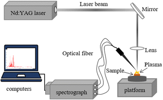
The LIBS acquisition device in this study was built by our laboratory, as shown in Fig. 1. The excitation source chosen for the device was a Q-switched Nd: YAG laser (DAWA300, Beijing LeiBao Photoelectric Technology Co., Ltd, China) with a pulse width of 8 ns, an excitation wavelength of 1064 nm and a repetition rate of 5 Hz, and a laser energy was 45 mJ. The rare earth ore sample press was first placed on a three-dimensional manually adjustable stage, and when the laser was applied to the surface of the rare earth ore sample through the lens, the plasma generated during the process was collected through a quartz collimating lens at 45° to the laser beam and transmitted via optical fiber to a three-channel spectrometer (Ocean Optics, MX2500+, America). Wavelength range of 200–550 nm, resolution of 0.07 nm, a delay time of 4.2 μs and door width of 2 ms, and LIBS spectral collection in ambient temperature and pressure. Ocean Optics MaxLIBS was used as the control software.

Fig. 1 Schematic diagram of LIBS spectrum acquisition.

LIBS spectra were collected by randomly selecting 20 different locations for each rare earth ore sample compression slice because of the heterogeneity of the rare earth ore samples. 25 LIBS spectra were collected for each rare earth ore sample, anomalous spectra were removed using Euclidean-distances, and the remaining spectra were averaged to obtain 25 spectra for 25 samples. 8 rare earth ore samples (#5, #9, #11, #14, #17, #21, #22 and #25) were manually selected as the prediction set for validating the PLS model performance, and the rest were used as the calibration set for constructing the PLS model.

2.3 Introduction of method and modeling process

iPLS (interval Partial Least Squares)³⁷ involves dividing the spectral data equally into small intervals of equal width, building a PLS model for each subinterval, and then filtering the optimal spectral bands based on the 5-fold cross validation results of the model. The variables used for modeling can be reduced compared to full spectral variable modeling.

VIP (Variable Importance Projection) is a PLS based method for selecting characteristic variables. In multiple linear regression problems, the projection of variable importance can be applied when the sample size is small or when there is a strong correlation between multiple independent variables in the sample. By calculating the integrated principal components of the independent variables, the explanatory power of the independent variables in relation to the corresponding dependent variables are derived, and the independent variables are screened according to this difference in explanatory power.

iPLS-VIP (interval Partial Least Squares combined with Variable Importance Projection) is a hybrid variable selection strategy. Firstly, the characteristic interval of spectrum is selected by iPLS, then the characteristic interval selected by iPLS further extracted by VIP, and the corresponding characteristic variables are obtained.

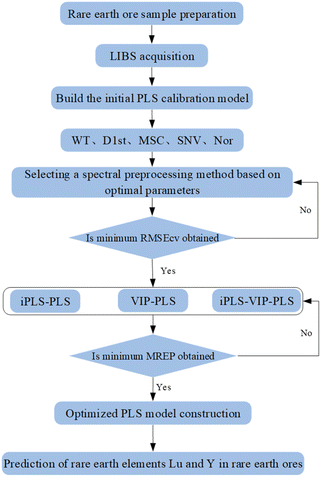
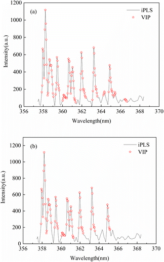
Fig. 2 shows the hybrid variable selection strategy combined with PLS model construction process for LIBS quantitative analysis of rare earth elements Lu and Y in rare earth ores. The main steps of the PLS algorithm for modeling LIBS spectral data of rare earth minerals include: (1) sample preparation of rare earth ores; (2) LIBS data acquisition; (3) constructing an initial PLS calibration model; (4) spectral pretreatment; (5) variable selection; (6) optimal PLS calibration model construction; (7) prediction of rare earth elements Lu and Y in rare earth ores. All the data processes were accomplished by MATLAB (Math Works, Version R2019b).

Fig. 2 The flow chart of the PLS model construction.

3. Result and discussion

3.1 LIBS spectral analysis

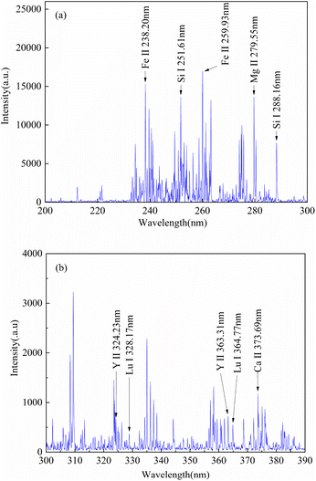
Fig. 3 shows the average LIBS spectra of 5# rare earth ore sample in the spectral region of 200–390 nm, and the characteristic spectral lines of Lu, Y, Fe, Ca, Si and Mg elements in iron ore samples were identified based on the National Institute of Standards and Technology (NIST) database,³⁸ and the characteristic spectral peaks identified were mainly Lu (328.17 nm, 364.77 nm), Y (324.23 nm, 363.31 nm), Fe (238.2 nm, 259.93 nm), Ca (373.69 nm), Si (251.61 nm, 288.16 nm) and Mg (279.55 nm).

Fig. 3 LIBS spectra of 5# rare earth ore samples ((a): 200–300 nm; (b): 300–390 nm).

3.2 Selection of pretreatment methods

As can be seen in Fig. 3, the LIBS spectra of rare earth ores were subject to spectral drift, spectral non-smoothness and noise. Spectral pre-processing can be used to filter out extraneous information from the spectra and reduced the interference of noise and spectral drift, and improved prediction performance of the model. Therefore, the effects of different preprocessing methods of normalization (Nor), standard normal variation (SNV), wavelet transform (WT), first order derivative (D1st) and multivariate scatter correction (MSC) on the PLS calibration model were investigated. The number of smooth points of the first derivative was optimized by 5-fold cross validation. Fig. 4 showed the effects of different smoothing points of the first derivative on the analysis ability of the PLS calibration model. It can be seen from Fig. 4 that for Lu, as the number of smooth points increases, the RMSECV value increased firstly and then decreased. When the number of smooth points was 9, the RMSECV was smallest at 3.3917 μg g⁻¹, and the R²cv was largest at 0.7819. At this time, the PLS calibration model had better predictability. For Y element. When the number of smoothing points was 11, the RMSECV was smallest, which was 310.2202 μg g⁻¹, and the R²cv was largest of 0.7703. At this time, the PLS calibration model had better prediction performance. The WT wavelet basis functions and the number of decomposition layers were optimized by 5-fold cross validation. Fig. 5 showed the effect of different wavelet basis functions and wavelet decomposition layers on the analytical capability of the PLS calibration model. As can be seen from Fig. 5, for Lu elements, RMESCV decreased firstly and then increased with the increase of decomposition layer numbers, when the wavelet function was db3 and decomposition layers was 2, the RMSECV was smallest, with 3.2755 μg g⁻¹, R²cv was maximum with 0.8025. At this time, PLS calibration model had a better prediction performance. For the Y element selection when the WT wavelet function was db2 and decomposition layer was 1, the RMSECV was smallest with 319.6993 μg g⁻¹ and the R²cv was largest with 0.8157. At this time, the PLS calibration model had a better prediction performance.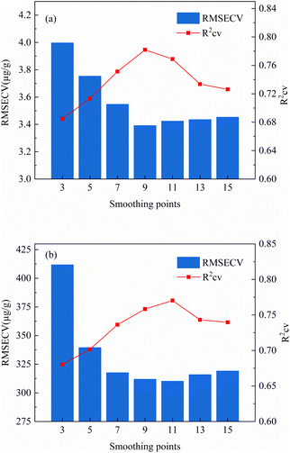

Fig. 4 The effect of different smoothing points of the first order derivative on the analytical ability of the PLS calibration model ((a): Lu; (b): Y).

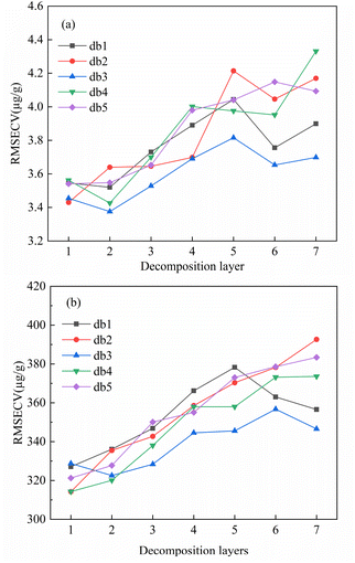Fig. 5 The effect of different wavelet basis functions and wavelet decomposition layers on the analytical capability of the PLS calibration model ((a): Lu; (b): Y).

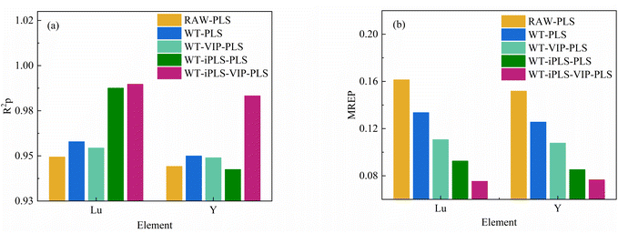
Fig. 6 showed the effects of different pre-processing methods of Nor, SNV, WT, D1st and MSC on the PLS calibration model were examined on the basis of the model parameters of the optimal spectral pre-processing method. The performance of the PLS calibration model built from the WT pre-treated spectra was improved compared to the original spectra. For the Lu element, R²cv was improved from 0.7732 to 0.8025, RMSECV was reduced from 3.5388 μg g⁻¹ to 3.2755 μg g⁻¹, and MREP for test set was reduced from 0.1614 to 0.1336. For Y element, R²cv was improved from 0.7965 to 0.8152, RMSECV was reduced from 333.2424 μg g⁻¹ decreased to 319.6993 μg g⁻¹ and the MREP for the test set decreased from 0.1518 to 0.1256.

Fig. 6 Influence of different pretreatment methods on the analytical ability of PLS calibration model ((a): Lu; (b): Y).

3.3 The effect of variable selection of PLS calibration models

For the WT preprocessed spectra, although the prediction performance of the PLS calibration model is slightly improved compared to the original spectra, there are still some redundant variables in the spectra that can reduce the prediction performance of the PLS calibration model. Therefore, variable selection is used to reduce redundant information in the spectra and improve the predictive performance of the PLS calibration model.

3.3.1 PLS calibration models based on iPLS. The spectra after WT treatment was divided into 9–25 intervals by iPLS method, PLS calibration model was established in each interval, and the best modeling interval was selected by RMSECV as the evaluation index. It can be seen from Table 2 that for the Lu element, when the number of separation intervals was 24, the RMSECV of the 14th interval used to establish the PLS calibration model was smallest, which was 1.2211 μg g⁻¹. The PLS calibration model of Lu element was established with the variables selected by iPLS, and the optimal Lv was 9 by 5-fold cross validation, of which R²p was 0.9876, RMSEP was 0.9436 μg g⁻¹, and MREP was 0.0926. For the Y element, when the number of separation intervals was 24, the RMSECV of the PLS calibration model established in the 14th interval was smallest, which was 126.5878 μg g⁻¹. Used the variables selected by iPLS to establish the PLS calibration model of the Y element, and used 5-fold cross validation to select the optimal Lv of 8, R²p of 0.9425, RMSEP of 142.0406 μg g⁻¹. Compared with the full-spectrum PLS calibration model after WT preprocessing, the prediction performance of the PLS calibration model was further improved by iPLS variable selection.

Table 2 R²cv and RMSECV of the iPLS model with different number of intervals corresponding to Lu and Y

Intervals	Lu			Y			Number of variables
	Interval number	R^2cv	RMSECV (μg g^−1)	Interval number	R^2cv	RMSECV (μg g^−1)
9	9	0.9436	2.4437	9	0.9419	247.7134	642
10	10	0.9462	2.3770	10	0.9448	240.5670	578
11	5	0.9453	2.6487	5	0.9464	260.5057	525
12	7	0.9787	1.5281	7	0.9760	162.0485	482
13	9	0.9411	2.5030	9	0.9390	256.3393	445
14	8	0.9770	1.5881	8	0.9740	168.4629	413
15	14	0.9151	2.9377	14	0.9177	290.5648	385
16	9	0.9758	1.6216	9	0.9715	175.5433	361
17	16	0.9360	2.5873	16	0.9378	256.6047	340
18	17	0.9286	2.7193	10	0.9708	178.9134	321
19	11	0.9809	1.4353	11	0.9804	146.1875	304
20	19	0.9387	2.5227	19	0.9416	247.6393	289
21	12	0.9813	1.4205	20	0.9549	217.5626	275
22	21	0.9572	2.1078	21	0.9552	216.3079	262
23	22	0.9600	2.0347	22	0.9577	209.9137	251
24	14	0.9871	1.2211	14	0.9862	126.5878	241
25	14	0.9716	1.7501	14	0.9689	183.4573	231

---

3.3.2 PLS calibration models based on VIP. The variable importance projection method is adopted to extract features from the spectral data after wavelet transform, and the variable importance threshold was optimized. As can be seen from Fig. 7, for Lu element, when the VIP threshold was 0.19, the RMSECV was smallest, which was 3.1715 μg g⁻¹, the R²cv was largest, which was 0.8198, the R²p of the prediction set was 0.9544, the RMSEP was 1.3481 μg g⁻¹, and the MREP was 0.1107, and the number of variables was 1468 at this time. For Y element, when the VIP threshold was 0.15, the RMSECV was smallest, which was 308.0653 μg g⁻¹, the R²cv was largest, which was 0.8319, the R²p of the prediction set was 0.9490, the RMSEP was 139.8618 μg g⁻¹, and the MREP was 0.1078, and the number of variables was 1820 at this time. With VIP variable selection, the predictive performance of the PLS calibration model was slightly improved compared to the full spectrum PLS calibration model preprocessed by WT.

Fig. 7 Optimization diagram of VIP variable importance threshold based on PLS calibration model ((a): Lu; (b): Y).

3.3.3 PLS calibration models based on iPLS-VIP. When iPLS selects the optimal wave band for modeling, there are some irrelevant variables in the selected wave band, while VIP selects the wave points of the full spectrum, but there are more features selected under the optimal threshold, which will increase modeling time. Therefore, this section studies the influence of iPLS-VIP hybrid variable selection on the prediction performance of the PLS calibration model. The optimal band selected by iPLS in Section 3.3.1 was used for variable selection by VIP to select the wave point, it can delete irrelevant variables, and retain useful information more comprehensively. Fig. 8 shows a graph of optimizing VIP variable importance threshold through 5-fold cross validation. It can be seen from Fig. 8 that when the VIP threshold was 0.4, the Lu element has better prediction performance, R²cv reached 0.9584, RMSECV was 1.4939 μg g⁻¹, the prediction set R²p reached 0.9897, the RMSEP was 0.8150 μg g⁻¹, and the MREP was 0.0754; When the VIP threshold was 0.6, the Y element had better prediction performance, R²cv reached 0.9554, RMSECV was 156.7039 μg g⁻¹, the test set R²p reached 0.9833, the RMSEP was 97.1047 μg g⁻¹, and the MREP was 0.0766. After implementing the hybrid variable selection method, the predictive error of the model was significantly reduced. Fig. 9 showed the wavelength points selected by iPLS-VIP method. These wavelength points were also a region where the feature peaks of Lu and Y were concentrated. However, the PLS calibration model based on these characteristic variables selected by iPLS-VIP had a relatively good prediction performance.

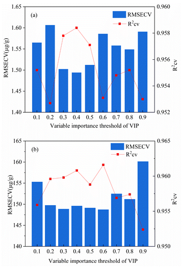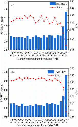
Fig. 8 Optimization diagram of iPLS-VIP variable importance threshold based on PLS calibration model ((a): Lu; (b): Y).

Fig. 9 Wavelength points selected based on the iPLS-VIP method. ((a): Lu, (b): Y).

3.3.4 Comparison of different PLS calibration models. This section compared the prediction performance of the PLS calibration model under different variable selection methods, and proved that it was feasible to select variables according to the idea of searching the wave band before selecting the wave point. As can be seen from Table 3, the optimal prediction performance for rare earth elements Lu and Y were obtained from a quantitative analysis model based on WT-iPLS-VIP-PLS. Compared with WT-iPLS-PLS and WT-VIP-PLS, WT-iPLS-VIP-PLS had a small improvement in 5-fold cross validation results, but the external validation results of WT-iPLS-VIP-PLS were better than WT-iPLS-PLS and WT-VIP-PLS. In addition, WT-iPLS-VIP-PLS selected fewer variables and took less time to model. As can be seen from Fig. 10, the predictive error of the model was significantly reduced, and the LIBS technique combined with the WT-iPLS-VIP-PLS calibration model provided better quantitative performance. In summary, the combination of iPLS and VIP can be used as a more effective method for variable selection, because the results were better than the other two variable selection methods. Fig. 11 showed the relationship between the reference and predicted values obtained by the WT-iPLS-VIP-PLS model. It can be seen from Fig. 11 that there was a better linear relationship between the predicted values and the reference values using the WT-iPLS-VIP-PLS calibration model to predict the eight prediction set samples. This study showed that the model had good predictive performance, enabling rapid quantitative analysis of rare earth elements Lu and Y in rare earth ores.

Table 3 Predictive performance of Lu and Y by different PLS calibration models

Elements	Calibration models	Lv	Number of variables	5-fold cross validation		Prediction set
				R^2cv	RMSECV (μg g^−1)	R^2p	RMSEP (μg g^−1)	MREP
Lu	RAW-PLS	7	5784	0.7732	3.5388	0.9494	1.7536	0.1614
	WT-PLS	9	5784	0.8025	3.2755	0.9579	1.5023	0.1336
	WT-VIP-PLS	11	1468	0.8178	3.2273	0.9544	1.3481	0.1107
	WT-iPLS-PLS	9	241	0.9517	1.6114	0.9876	0.9436	0.0926
	WT-iPLS-VIP-PLS	7	113	0.9584	1.4939	0.9897	0.8150	0.0754
Y	RAW-PLS	8	5784	0.7965	333.2424	0.9442	175.1057	0.1518
	WT-PLS	11	5784	0.8157	319.6993	0.9500	157.0477	0.1256
	WT-VIP-PLS	10	1820	0.8242	313.0468	0.9490	139.8618	0.1078
	WT-iPLS-PLS	8	241	0.9551	156.0450	0.9425	142.0406	0.0853
	WT-iPLS-VIP-PLS	7	85	0.9616	148.7193	0.9833	97.1047	0.0766

---

Fig. 10 Predictive performance of different PLS calibration models ((a): R²p; (b): MREP).

Fig. 11 The relationship between the reference value and predictive value obtained by iPLS-VIP-PLS calibration model ((a): Lu, (b): Y).

4. Conclusions

In this study, PLS calibration model combined with LIBS was successfully applied for rapid quantitative analysis of rare earth elements Lu and Y in rare earth ores. The results showed that the WT-iPLS-VIP-PLS calibration model had the best prediction performance with the R² = 0.9897, RMSE = 0.8151 μg g⁻¹, MRE = 0.0754 and R² = 0.9833, RMSE = 97.1047 μg g⁻¹, MRE = 0.0766, for Lu and Y elements in the prediction set, respectively. Compared with the PLS calibration model based on the original spectrum, the MRE of Lu and Y in PLS calibration model based on the iPLS-VIP decreased 8.6% and 7.5%, respectively. It shows that the hybrid variable selection method is helpful to improve the calculation efficiency and prediction performance of the model. The research showed that LIBS technology combined with WT-iPLS-VIP-PLS was an effective method to detect rare earth elements in rare earth ores. In the future, with the further development and perfection of technology, the application of LIBS technology in the field of geological exploration will be more extensive. This study provides theoretical basis and technical reference for the future application of LIBS technology to in situ rapid and accurate quantitative analysis in more geological exploration fields.

Author contributions

Xiangqian Liu: methodology, software, investigation, experiment, data collection, and writing–original draft preparation. Chunhua Yan: methodology, software, and investigation. Duanyang An: experiment and data collection. Chengen Yue: software and methodology. Tianlong Zhang: funding acquisition, writing review & editing. Hongsheng Tang: funding acquisition, supervision, and writing-review & editing. Hua Li: funding acquisition, supervision, and project administration.

Conflicts of interest

There are no conflicts to declare.

Acknowledgements

This work was supported by the National Natural Science Foundation of China (No. 22173071); Scientific Research Program Funded by Shaanxi Provincial Education Department (No. 22JP064); Natural Science Basic Research Program of Shaanxi (No. 2023-JC-QN-0169).

References

1. W. N. Shi, S. F. Yang and J. S. Li, Sci. Rep., 2018, 8, 4830.
2. A. S. Yurtaeva, T. P. Sorokina, K. S. Plekhova, O. V. Potapenko, T. I. Gulyaeva, V. P. Talsi and V. P. Doronin, Pet. Chem., 2021, 61, 325–331.
3. T. I. Kostelnik and C. Orvig, Chem. Rev., 2019, 119, 902–956.
4. O. Sartor, J. de Bono, K. N. Chi, K. Fizazi, K. Herrmann, K. Rahbar, S. T. Tagawa, L. T. Nordquist, N. Vaishampayan, G. El-Haddad, C. H. Park, T. M. Beer, A. Armour, W. J. Perez-Contreras, M. DeSilvio, E. Kpamegan, G. Gericke, R. A. Messmann, M. J. Morris, B. J. Krause and V. Investigators, N. Engl. J. Med., 2021, 385, 1091–1103.
5. J. Y. He, Q. Yu, Y. P. Zhou, Y. W. Wang and F. Long, J. Wuhan Univ. Technol., Mater. Sci. Ed., 2020, 35, 248–355.
6. S. Zhang, S. E. Saji, Z. Y. Yin, H. B. Zhang, Y. P. Du and C. H. Yan, Adv. Mater., 2021, 33, 2005988.
7. Y. A. Cui, Y. H. Wang, Z. Y. Cui, W. L. Qi, J. D. Wang, P. F. Ju, Y. Zhao, B. Liu, T. Zhang and F. H. Wang, Materials, 2020, 13, 3651.
8. C. R. Bhatt, J. C. Jain, C. L. Goueguel, D. L. McIntyre and J. P. Singh, Appl. spectrosc., 2018, 72, 114–121.
9. M. F. Attallah, F. S. Abdou and H. F. Aly, Radiochim. Acta, 2021, 109, 225–232.
10. J. C. Farinas, I. Rucandio, M. S. Pomares-Alfonso, M. E. Villanueva-Tagle and M. T. Larrea, Talanta, 2016, 154, 53–62.
11. Y. B. Zhu, Talanta, 2020, 209, 120536.
12. H. T. Mnculwane, Analytica, 2022, 3, 135–143.
13. E. De Pauw, P. Tack, M. Lindner, A. Ashauer, J. Garrevoet, B. Vekemans, G. Falkenberg, F. E. Brenker and L. Vincze, Anal. Chem., 2019, 92, 1106–1113.
14. Z. A. Arp, D. A. Cremers, R. C. Wiens, D. M. Wayne, B. Sallé and S. Maurice, Appl. spectrosc., 2004, 58, 897–909.
15. T. X. Phuoc, P. Wang and D. McIntyre, Fuel, 2016, 163, 129–132.
16. T. T. Chen, T. L. Zhang and H. Li, TrAC, Trends Anal. Chem., 2020, 133, 116113.
17. K. Singh Vivek, J. Sharma, K. Pathak Ashok, T. Ghany Charles and M. A. Gondal, Biophys. Rev., 2018, 10, 1221–1239.
18. Z. Q. Yue, C. Sun, F. Y. Chen, Y. Q. Zhang, W. J. Xu, S. Shabbir, L. Zou, W. G. Lu, W. Wang, Z. W. Xie, L. Y. Zhou, Y. Lu and J. Yu, Biomed. Opt. Express, 2021, 12, 2559–2574.
19. Y. P. Xie, J. Wang, Y. C. Hu, J. Zhang, Y. Gao, H. P. Li and S. Wang, Appl. Surf. Sci., 2021, 566, 150709.
20. G. Kim, J. Kwak, J. Choi and K. Park, J. Agric. Food Chem., 2012, 60, 718–724.
21. Z. Abdel-Salam, S. M. I. Alexeree and M. A. Harith, Spectrochim. Acta, Part B, 2018, 149, 112–117.
22. J. Agresti, C. Indelicato, M. Perotti, R. Moreschi, I. Osticioli, I. Cacciari, A. A. Mencaglia and S. Siano, Molecules, 2022, 27, 1813.
23. G. S. Senesi, B. Campanella, E. Grifoni, S. Legnaioli, G. Lorenzetti, S. Pagnotta, F. Poggialini, V. Palleschi and O. De Pascale, Spectrochim. Acta, Part B, 2018, 143, 91–97.
24. W. Zhao, C. Li, C. Yan, H. Min, Y. An and S. Liu, Anal. Chim. Acta, 2021, 1166, 338574.
25. T. F. Akhmetzhanov and A. M. Popov, J. Anal. At. Spectrom., 2022, 37, 2330–2339.
26. M. Martin, R. C. Martin, S. Allman, D. Brice, A. Wymore and N. Andre, Spectrochim. Acta, Part B, 2015, 114, 65–73.
27. C. R. Bhatt, F. Y. Yueh and J. P. Singh, Appl. Opt., 2017, 56, 2280.
28. S. Banu, U. Aslıhan, B. I. Hakki and K. Hamit, J. Cereal Sci., 2022, 104, 103435.
29. J. Qi, T. Zhang, H. Tang and H. Li, Spectrochim. Acta, Part B, 2018, 149, 288–293.
30. Y. Ding, W. Zhang, X. Q. Zhao, L. W. Zhang and F. Yan, J. Anal. At. Spectrom., 2020, 35, 1131–1138.
31. M. G. Li, H. Fu, Y. Du, X. Huang, T. L. Zhang, H. S. Tang and H. Li, J. Anal. At. Spectrom., 2022, 37, 1099–1108.
32. M. S. Babu, Neelmani, N. J. Vasa, R. Sarathi and T. Imai, Meas. Sci. Technol., 2021, 32, 115201.
33. J. Tang, Y. Tian, P. Zhang and X. Liu, IEEE Trans. Neural Networks Learn. Syst., 2018, 29, 3463–3477.
34. C. R. Guan, T. Y. Wu, J. W. Chen and M. Li, Chemosensors, 2022, 10, 490.
35. C. H. Yan, J. Liang, M. J. Zhao, X. Zhang, T. L. Zhang and H. Li, Anal. Chim. Acta, 2019, 1080, 35–42.
36. X. K. Li, Z. Y. Li, Z. Y. Yang, D. Qiu, J. M. Li and B. Q. Li, Spectrochim. Acta, Part A, 2022, 275, 121–123.
37. N. Rethfeldt, P. Brinkmann, D. Riebe, T. Beitz, N. Köllner, U. Altenberger and H. G. Löhmannsröben, Minerals, 2021, 11, 1379.
38. https://www.physics.nist.gov/PhysRefData/Handbook/periodictable.htm.

---