DOI:
10.1039/D4AN00965G
(Paper)
Analyst, 2024,
149, 5455-5462
A simple spectrogram model for high-accuracy spectral calibration of VIPA spectrometers
Received
9th July 2024
, Accepted 12th September 2024
First published on 13th September 2024
Abstract
The virtually imaged phased array (VIPA) spectrometer uses the orthogonal dispersion method and has the advantages of compact structure, high spectral resolution, and wide wavelength coverage. It has been widely used in different fields. However, due to the non-linear dispersion of the VIPA etalon and the cross-dispersion structure of the VIPA spectrometer, simple and high-accuracy wavelength calibration remains a challenge. In this paper, a new and simple five-parameter spectrogram model is developed by simplifying the phase-matching equation of the VIPA etalon and considering the angle between the camera and dispersion direction, which can achieve a frequency accuracy better than one pixel. The performance of the model is demonstrated by measuring the CO2 absorption spectrum in the range of 1.42 to 1.45 μm using a self-designed near-infrared VIPA spectrometer  . The reported method is simple and easy to solve with high accuracy, which is conducive to promoting the application of VIPA spectrometers in precision measurement.
Introduction
Ultra-high resolution  spectroscopy has important applications in many fields, such as multispecies trace gas detection,1,2 molecular fingerprinting,3 precision measurement,4 spectral-domain optical coherence tomography,5,6 astronomical observation,7 and basic physics and chemistry.8,9 Over more than a decade, a new ultra-high-resolution spectrometer based on the virtually imaged phased array (VIPA) etalon has become an exciting topic in the field of broadband spectroscopy research.3 The VIPA spectrometer uses the orthogonal dispersion structure composed of the VIPA etalon and grating to achieve two-dimensional light dispersion, and uses an area-array camera to collect the light, achieving high-resolution
  broadband spectral measurements (from about 9 nm in the visible band to 90 nm in the mid-infrared band in a single frame);3,7,8 using a high-speed camera, microsecond time-resolved (or even faster) broadband spectral measurements can be achieved,8,9 which has great application potential. However, due to the non-linear dispersion of the VIPA etalon and the cross-dispersion structure of the spectrometer, high accuracy wavelength calibration of VIPA spectrometers using a simple calibration setup remains a challenge.10
Currently, wavelength calibration of the VIPA spectrometer is usually done by two methods: one is using a high-precision optical frequency reference (HPOFR), such as a tunable laser,11 a frequency comb,3,12,13 an F–P etalon,5,6 or an optical spectrum analyzer (OSA)10,14 to calibrate the frequency. For example, Diddams et al. used a single-longitudinal mode laser to provide an absolute frequency reference;3 Zhu et al. used a frequency comb to provide a relative frequency reference, achieving an extremely high accuracy of about 0.03 pixels.15 The other method is using the absorption spectrum of molecules or the absorption or emission spectrum of atoms to fit the parameters of the dispersion model, such as the orthogonal dispersive model,14 proportional model16 and linear model.16 The dispersion model can establish the relation between the pixel coordinates and the wavelengths of the entire spectral image. For example, Thrope et al. used the gas absorption data (CO2, H2O, CH4 and NH3) and the orthogonal dispersive model14 of the VIPA spectrometer to obtain a high accuracy mapping of pixel to wavelength in the range of 1.5 to 1.7 μm.1 Klose et al. used a third-order polynomial fit of the experimental peak position to the theoretical peak from the HITRAN database to achieve wavelength calibration.17 These kinds of methods are easy to integrate into the detection system and realize real-time calibration, and the setup is simpler than that of the HPOFR method. However, due to the deviation between the ideal model and the actual structure, the accurate solution of the parameters is challenging.
In this work, we report the development of a new spectrogram model to achieve high accuracy wavelength calibration. By replacing the optical path difference (OPD) in the phase-matching equation of the VIPA etalon10 with a low-order polynomial function, the number of parameters of the model is reduced and the conversion between pixel coordinates and spatial positions is elided, making the solving of parameters easier. By adding the angle between the dispersion direction and the camera, the model is more applicable. Similar approaches have been used in some HPOFR applications16,18 and in the calibration of an échelle spectrometer,19–21 where sub-pixel calibration accuracy can be achieved. Here, a more general approach than the orthogonal dispersive model has been developed, which enables high accuracy calibration in absorption applications without any additional calibration setup like a single-mode laser, an F–P etalon or others. The performance of the technique is demonstrated on a self-designed near-infrared VIPA spectrometer  with a CO2 absorption range of 1.42–1.45 μm. By comparing the theoretical coordinates calculated using the spectrogram model and the centroid coordinates of the measured image, an average accuracy of better than 1 pixel is achieved.
Principle of VIPA spectrometers
The traditional dispersion model
In an ideal VIPA-grating spectrometer, the traditional dispersion model (spatial (x, y) and wavelength dependence of the intensity distribution) can be expressed as the product of the grating and the VIPA etalon distributions:6,14| |  | (1) |
where the first product term Iin(λ) is the input beam power spectral density, the second term exp(−2fc2y2/f2W2) is the envelope of the light intensity along the y direction, the third term represents the VIPA dispersion law, and the fourth term describes the grating dispersion. fc and f are the focal lengths of the cylindrical lens and the imaging lens, respectively. r1 and r2 are the reflection coefficients of the front and back surfaces of the VIPA etalon, respectively. d, θig and θd are the grating constant, incident angle and diffraction angle, respectively. λ0 and W are the central wavelength and the waist radius of the collimated beam, respectively. OPD = mλ is the optical path difference between adjacent beams of the VIPA etalon.
For different VIPA interference orders (m), the phase-matching equation in the vertical direction can be written as follows:14
| |  | (2) |
where
ne,
t,
θi and
θin are the refractive index, thickness, incident angle and refraction angle of the VIPA etalon, respectively, and the relationship between
ne,
θi and
θin is
θin ≈
θi/
ne.
In the horizontal direction, the dispersion is caused only by the grating, and the phase-matching equation can be expressed as follows:19–21
| | mgratingλ = d(sin![[thin space (1/6-em)]](https://www.rsc.org/images/entities/char_2009.gif) θig ± sinθd) θig ± sinθd) | (3) |
| |  | (4) |
where
mgrating is the diffraction order, which is +1 in most cases in VIPA spectrometers.
The spectrogram model
For the spectrogram model, there is only one spatial position variable (y) in the OPD expression in the VIPA dispersion direction. The phase-matching equation for the VIPA etalon can be modified as follows:| |  | (5) |
where Yp is the vertical coordinate of the pixel, m is the VIPA dispersion order at wavelength λYp, and a0, a1, and a2 are the coefficients of the second-order polynomial.
In the grating dispersion direction, each fringe represents a VIPA interference order within one VIPA FSR. Therefore, the relationship between the interference order m and a series of coordinates Xp on the fringe can be determined by the fringe recognition algorithm,22 as shown in the following equation:
| |  | (6) |
where
Xp is the horizontal coordinate and
b0 and
b1 are the one-order polynomial coefficients.
Fig. 1(a) shows an ideal schematic spectrogram of a broadband light source and four beams of single longitudinal mode light (wavelengths are λ0 to λ3). For a light beam of a specified frequency, such as λ2, there are multiple light spots (red, 3 in this figure) along the VIPA dispersion direction, which are distributed on different fringes, representing different interference orders of the VIPA etalon. For two beams with the same dispersion angle in the y direction, such as λ2 and λ3, the light spots are separated into different fringes by the grating.
 |
| | Fig. 1 The schematic spectrogram of a broadband light source and four beams of single longitudinal mode light (wavelengths are λ0 to λ3). (a) Ideal spectrogram model; (b) rotated spectrogram model. (c) The zoomed-in view of the rotated spectrogram model. The ellipses represent the spots of different single-mode light. In the vertical direction, different wavelengths (in different colours) are separated by the VIPA etalon. Different positions of the same wavelength represent different VIPA interference orders. In order to obtain a wider spectral coverage, a grating is used to separate the VIPA overlapping orders to form a fringe pattern. The region of one VIPA FSR can be roughly determined by a characteristic wavelength (such as λ2). Then the fringes are connected end-to-end in the direction of the black arrows to obtain a one-dimensional spectrum. γ represents the angle between the VIPA dispersion direction and the y-axis of the camera. | |
The above are all ideal results. In actual spectrometers, even if the installation error is quite small, special optical design and aberration19,23 will affect the relationship between the wavelength and pixel coordinates, resulting in a certain gap between the spectrum image collected by the spectrometer camera and the ideal image. For example, Diddams et al.3 and Zhou et al.24 reported the camera rotation method, which rotated the camera that caused the coordinate axis to differ in the dispersion direction (as shown in Fig. 1(b)). To solve this problem, the model can be updated by simply adding the parameter γ (the angle between the VIPA dispersion direction and the camera y-axis).
Among the influence of aberrations, according to the third-order aberration theory, only distortion aberration25 will affect the shape of the image, thereby affecting the interference position of a certain wavelength in the orthogonal dispersion system, causing bending of fringes, while other aberrations such as spherical aberration and coma aberration only affect the spectral resolution and fringe width of the spectrometer. In the cases of a large distortion effect,13 the spectral image can be corrected by using techniques such as the distortion correction algorithm.27 Due to the small size of the VIPA etalon (which is comparable to the size of the F–P etalon) and the grating, the field of view of the imaging system of the VIPA spectrometer is small, and its distortion aberration can generally be ignored.26 Therefore, in practical applications, the spectrogram model can be used for the wavelength calibration of the VIPA spectrometer.
Spectral calibration algorithm
The process of the spectral calibration algorithm based on the spectrogram model is shown in Fig. 2. To achieve a high-accuracy calibration, multiple wavelengths and their corresponding pixel coordinates of different VIPA interference orders are required. Here, we use Nugent-Glandorf's method24 to obtain the wavelengths of these absorption spots. Then the parameter γ is determined from these inputs. In the ideal spectrogram, the x-coordinate Xp is determined only by the grating dispersion, and the y-coordinate Yp is determined only by the VIPA dispersion. Thus, γ can be determined by the following formula:| |  | (7) |
where i is the number of absorption spots, (Xi, Yi) is the pixel coordinate of a collected image and (Xpi, Ypi) is the pixel coordinate of the corresponding ideal image. The conversion equation between the pixel coordinates (Xi, Yi) and (Xpi, Ypi) is as follows:28| |  | (8) |
where (Tx, Ty) is the coordinate of the rotation center.
 |
| | Fig. 2 Algorithm flow chart for the spectral calibration of the VIPA spectrometer. | |
After determining the angle γ, the next step is to establish an ideal model input. As shown in Fig. 1, assuming that the VIPA interference order of one of the fringes is m, and the adjacent orders are m ± 1. The matrix (X, Y, m, λ) of the spectral image and the corresponding matrix (Xp, Yp, m, λ) of the spectrogram model can be determined. With the coordinates (Yp, m, λ) as the ideal model input, the VIPA interference order m and the second-order polynomial parameters a0, a1 and a2 can be derived using the least-squares fitting method, as shown in the following formula:
| |  | (9) |
The (m, Yp, λ) relationship of other pixels on the fringes can be calculated using eqn (5). The model in the horizontal direction is similar to that in the vertical direction. In particular, for broadband input light, the x-coordinate of each central pixel on the fringes (Xm, m) can be directly obtained by the fringe recognition algorithm.22 Finally, the (X, Y, λ) relationship is determined using (m, Yp, λ), (Xp, m) and angle γ.
Experimental setup
The schematic diagram of the experimental setup for CO2 absorption spectroscopy is shown in Fig. 3. The experimental laser was a fiber output supercontinuum source (SC-5, YLS Photonics, with a wavelength range of 470 to 2400 nm). The output light was collimated using a fiber collimator and then selected by two filters to have a wavelength range of 1425 to 1450 nm (6900 to 7018 cm−1) for CO2 absorption detection. The filtered light was coupled into the Chernin gas cell, which consisted of five plano-concave mirrors, each with a radius of 0.5 m and an optical path length of 4 m. The output beam of the gas cell was sent to the self-designed VIPA spectrometer.29
 |
| | Fig. 3 The schematic diagram of the experimental setup. Filters are not shown in the figure. | |
The fiber-coupled input of the VIPA spectrometer was launched into free space and line-focused onto the entrance window of the VIPA etalon (free spectral range, FSR ∼ 60 GHz) using a cylindrical lens (fc = 100 mm). An orthogonally oriented reflective diffraction grating (GH25-24V, Thorlabs, 1200 lines per mm) was used to separate the overlapping orders. The two-dimensionally dispersed light was imaged onto the camera using a plano-convex imaging lens (f = 200 mm). The maximum distortion aberration of this type of imaging system is about 8 μm (less than 1 pixel), which is estimated using Zemax. The camera (LD-SW640, Leading Optoelectronic) had a pixel array of 640 × 512 with a pixel pitch of 15 μm and a maximum full frame rate of 23 Hz. The camera was slightly rotated to align the fringes with the camera's y-axis.
Results and discussion
Wavelength calibration of the VIPA spectrometer
The relationship between (X, Y) and λ of selected spots.
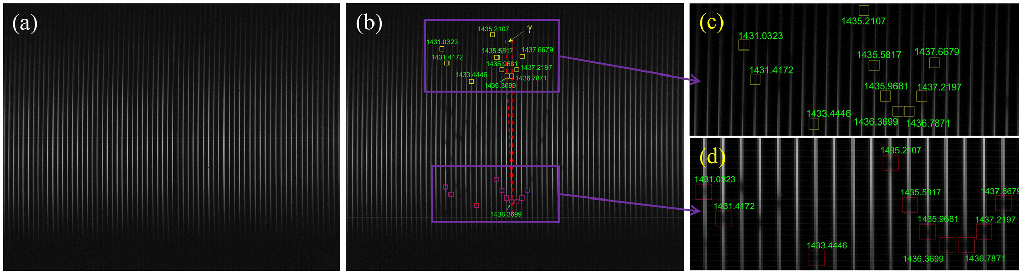
In this paper, a CO2 absorption spectrum was used as the model input to achieve high-precision spectral calibration. Pure N2 (99.999%) and pure CO2 (99.999%) were introduced into the gas cell to obtain the absorption spectrum. The cell pressure was stabilized at 200 mbar, and the temperature was 296 K. The collected images are shown in Fig. 4 ((a) is the N2 background image (I0) and (b) is the CO2 signal image (I)). The dark image (Id) was also collected.
 |
| | Fig. 4 Spectral images collected by the VIPA spectrometer. (a) The background image I0 of pure N2 and (b) the signal image I of pure CO2. (c) The zoomed-in view of one VIPA FSR in figure b and (d) the zoomed-in view of another VIPA FSR. The yellow squares represent the absorption spots given in Table 1. Yellow and pink represent different VIPA FSR regions, in a one-to-one correspondence. According to the Beer–Lambert law, the absorption image can be obtained by −ln[(I − Id)/(I0 − Id)]. | |
The theoretical spectral coverage of the VIPA spectrometer was around 1425–1450 nm at an 85-degree grating incidence angle.29 Since N2 has no absorption in this region, the fringes in Fig. 4(a) are continuous and can be used as the absorption baseline. The black spots in Fig. 4(b) were caused by CO2 absorption. The periodicity of these absorption spots can be used to identify different VIPA interference orders.1,16 By connecting these fringes end-to-end within one VIPA interference order, a one-dimensional spectrum without frequency axis calibration can be obtained. Using Klose's method,22 the wavelengths corresponding to the central pixels of these CO2 absorption spots were obtained. In this paper, a portion of the data was used to fit the spectrogram model, and the rest was used as a control group to evaluate the accuracy of the wavelength calibration. The center pixel coordinates and their corresponding wavelengths used for the model inputs are shown in Table 1 and marked in Fig. 4(b).
Table 1 Coordinates of the absorption spot's central for different VIPA interference orders used to determine the γ angle. Columns (a) and (b) correspond to the yellow and pink squares in Fig. 4(b), respectively
| Wavelength (nm) |
(a) Coordinate of one interference order (X, Y) |
(b) Coordinate of another interference order (X, Y) |
| 1437.6679 |
(334, 103) |
(343, 358) |
| 1437.2197 |
(324, 129) |
(333, 373) |
| 1436.7871 |
(314, 141) |
(324, 380) |
| 1436.3699 |
(305, 141) |
(314, 380) |
| 1435.9681 |
(295, 129) |
(304, 373) |
| 1435.5817 |
(286, 105) |
(295, 359) |
| 1435.2107 |
(278, 62) |
(285, 337) |
| 1433.4446 |
(238, 151) |
(247, 387) |
| 1431.4172 |
(191, 116) |
(199, 366) |
| 1431.0323 |
(182, 89) |
(189, 352) |
The input matrix (m, Yp, λ) of the ideal model.
As shown in Fig. 4(b), the deviation of adjacent orders is about 9 pixels. Since the different VIPA interference orders of the same wavelength have the same x-coordinates in the ideal spectrogram model, the parameter γ can be determined using eqn (7). Taking the angle γ as the independent variable and 1 × 10⁻⁴ degrees as the iteration step size, the total differences of the rotated x-coordinates were calculated. The angle γ with the minimum total difference is −2.0293 degrees. The 21st fringe from the left to right in Fig. 4(b) is selected for analysis. Its VIPA order is set to m. The obtained rotated coordinates and their corresponding VIPA orders that can be used in the spectrogram model are shown in Table 2.
Table 2 Coordinates and rotated coordinates of absorption spots used in the spectrogram model
| Wavelength (nm) |
VIPA order |
Center coordinate (X, Y) |
Corrected coordinate (Xp, Yp) |
| 1437.6679 |
m – 16 |
(343, 358) |
(320.8421, 381.0921) |
| 1437.2197 |
m – 15 |
(333, 372) |
(310.3526, 394.7292) |
| 1436.7871 |
m – 14 |
(324, 380) |
(300.0756, 402.3701) |
| 1436.3699 |
m – 13 |
(314, 380) |
(291.0813, 402.0514) |
| 1435.9681 |
m – 12 |
(304, 373) |
(281.3354, 394.7017) |
| 1435.5817 |
m – 11 |
(295, 359) |
(272.8368, 380.3918) |
| 1435.2107 |
m – 10 |
(285, 337) |
(263.6221, 358.0515) |
| 1433.4446 |
m – 5 |
(238, 151) |
(223.2380, 170.5038) |
| 1431.4172 |
m – 1 |
(199, 366) |
(176.6491, 383.9880) |
| 1431.0323 |
m – 0 |
(189, 352) |
(167.1512, 369.6427) |
Fitting of the model parameters.
The accuracy of the spectral calibration algorithm depends on the number of feature spots and their location in the spectrogram image. Although the spectrogram model theoretically only requires three feature wavelengths to achieve the second-order polynomial fit, in practical applications, generally speaking, the more feature spots there are and the wider their distribution in the y-axis direction, the higher is the calibration accuracy. Here, we first used 37 different feature spots to achieve high accuracy fitting. Then, we used different numbers and combinations of feature spots as model inputs and compared the fitting results. It was found that for an accurate fitting of model parameters, it is ideal to have 10 or more feature spots spread broadly (such as Table 2) as the model inputs.
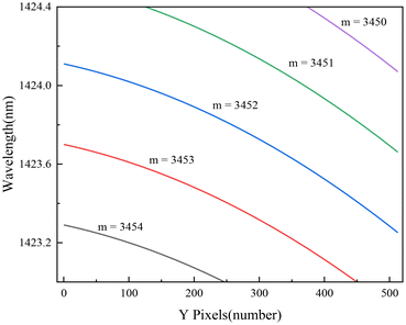
According to eqn (5), mλ (OPD) and the pixel vertical axis Yp satisfy a quadratic polynomial (mλ = OPD = a2Yp2 + a1Yp + a0).16 Therefore, the closer the assumed value of m is to the real VIPA interference order, the smaller the quadratic polynomial fitting residual between mλ and Yp. Using the parameter m as an independent variable, the least-squares method is used to fit mλ and Yp. The fitting residual can be expressed as follows:
| |  | (10) |
where
n is the number of input relationships (
λ and pixel coordinate).
Fig. 5(a), (b), and (c) show the second-order polynomial fitting results of the corrected y-coordinates and mλ values of 37 absorption spots for three different m values (3413, 3454, and 3493), respectively. Fig. 5(d) shows the total residuals under different m values (from 3400 to 3500). The total residuals were down and then up, which illustrates that the m value approaches the real VIPA interference order first and then away. When m = 3454, the fitting residual is the smallest, which represents the real order of the 21st fringe being 3454. Under this condition, the parameters a2, a1 and a0 of the second-order polynomial are −0.00647, −2.3535 and 4944539.5519, respectively.
 |
| | Fig. 5 Schematic diagram of the inversion of optimized model parameters. The second-order polynomial fitting results under the conditions of (a) m = 3413, (b) m = 3454, and (c) m = 3493. (d) The sum of the fitting residuals at different m values. | |
Relationship between (X, Y) and λ over the entire absorption image.
The same fringe recognition algorithm as Nugent-Glandorf et al.'s22 was used to obtain the central pixel coordinates of the fringes in images I and I0. Their corresponding coordinates were calculated using eqn (8) to obtain the matrix (X, Y, m) and the corresponding rotated matrix (Xp, Yp, m). Fig. 6 shows the theoretical spectrum calculated with the fitting parameters and different m values. The matrix (Yp, m, λ) can be obtained from the curve. The one-to-one relationship between these three matrices allows us to determine the wavelength (λ) of each central pixel (X, Y) on the fringes in images I and I0. The wavelengths of the absorption spots within one VIPA FSR were labeled as shown in Fig. 7.
 |
| | Fig. 6 Theoretical spectrum calculated by fitting parameters with different m values. Different lines (different m values) represent different fringes on the detector plane. The X coordinate of the pixel can be obtained by the fringe recognition algorithm. The Y coordinate of the pixel and its wavelength can be obtained from the curve, and thus the wavelength corresponding to each central pixel on the fringe can be obtained. | |
 |
| | Fig. 7 Zoomed-in CO2 absorption image. Absorption spots within a VIPA FSR are labelled with their wavelength. | |
The accuracy of the spectrogram model
In general, the centroid of light spots in the measured spectrogram is regarded as the position corresponding to the absorption line.23 To verify the accuracy of the spectrogram model, the centroid coordinates of some absorption peaks (including the absorption spots that are not involved in model parameter fitting) were calculated and compared with the peak coordinates calculated using the spectrogram model. The comparison results of 36 CO2 absorption lines are shown in Fig. 8, where the red and green points represent the error of the x-coordinate and the y-coordinate, respectively. The results show that the maximum calibration error is less than 2 pixels and the average error is about 1 pixel. Using the linear dispersion equation of the VIPA etalon,10 the maximum frequency error can be calculated to be 2.6 pm and the average frequency error is 0.88 pm. Compared to the deviation of the proportional model (∼20 pm)16 and the linear model (∼6 pm),16 the accuracy of the spectrogram model is better. Compared to the orthogonal dispersive model, although the accuracy is similar, the spectrogram model is more concise and easier to solve.
 |
| | Fig. 8 The errors of the spectrogram model. The red point represents the error in the X direction and the green point represents the error in the Y direction. | |
Since the fringe recognition algorithm can offset the effect of distortion to a certain extent,21 the deviation in the y-direction is larger than that in the x-direction. It is expected that the calibration accuracy can be improved to the sub-pixel level by combining distortion correction algorithms. In addition, it is expected that self-calibration can be further achieved by adding compensation functions (such as the method of Shen et al.19) or automatically calculating the deviation (such as the method of Sadler et al.30). Therefore, the spectrogram model is a promising technique that will play an important role in the applications of VIPA spectrometers.
Conclusion
In this work, a new simple, easy-to-solve and accurate spectrogram model calibration algorithm was developed for the wavelength calibration of VIPA spectrometers. The method simplified the dispersion model into 5 parameters and further considered the angle direction. The average accuracy was better than 1 pixel, which corresponds to a frequency accuracy of 0.88 pm. By combining with the distortion correction algorithm, the accuracy can be further improved. The reported method provides a useful tool for precision measurements.
Author contributions
HZ: investigation, methodology, and writing – original draft. WXZ: conceptualization, resources, supervision, and writing – review & editing. WHC and BXL: validation. FB, NNY and GFX: data curation. WJZ, LHD and WDC: resources and review. All authors contributed to discussions and the final version of the manuscript.
Data availability
All data are presented in the manuscript, and the files are available from the authors upon request.
Conflicts of interest
The authors declare no conflicts of interest.
Acknowledgements
The authors thank Dr. Dean S. Venables in University College Cork for his helpful discussions of this manuscript. The authors thank the National Natural Science Foundation of China (U21A2028), the Youth Innovation Promotion Association CAS (Y202089), and the HFIPS Director's Fund (YZJJ202101, BJPY2023A02) for financial support.
References
- M. J. Thorpe, D. Balslev-Clausen, M. S. Kirchner, J. Ye, K. D. Moll, R. J. Jones, B. Safdi and J. Ye, Opt. Express, 2008, 16, 2387–2397 CrossRef PubMed.
- K. C. Cossel, E. M. Waxman, I. A. Finneran, G. A. Blake, J. Ye and N. R. Newbury, J. Opt. Soc. Am. B, 2017, 34, 104–128 CrossRef PubMed.
- S. A. Diddams, L. Hollberg and V. Mbele, Nature, 2007, 445, 627–630 CrossRef PubMed.
- X. Zhu and J. He, J. Opt., 2019, 21, 025703 CrossRef.
- W. Bao, Z. Ding, P. Li, Z. Chen, Y. Shen and C. Wang, Opt. Express, 2014, 22, 10081–10090 CrossRef PubMed.
- C. Wang, Z. Ding, S. Mei, H. Yu, W. Hong, Y. Yan and W. Shen, Opt. Lett., 2012, 37, 4555–4557 Search PubMed.
- X. Zhu, D. Lin, Z. Zhang, X. Xie and J. He, Astron. J., 2023, 165, 228 CrossRef.
- A. J. Fleisher, B. J. Bjork, T. Q. Bui, K. C. Cossel, M. Okumura and J. Ye, J. Phys. Chem. Lett., 2014, 5, 2241–2246 CrossRef PubMed.
- B. J. Bjork, T. Q. Bui, O. H. Heckl, P. B. Changala, B. Spaun, P. Heu, D. Follman, C. Deutsch, G. D. Cole, M. Aspelmeyer, M. Okumura and J. Ye, Science, 2016, 354, 444–448 CrossRef PubMed.
- S. Xiao, A. M. Weiner and C. Lin, IEEE J. Quantum Electron., 2004, 40, 420–426 CrossRef.
- S. Xiao and A. M. Weiner, IEEE Photonics Technol. Lett., 2005, 17, 372–374 Search PubMed.
- S. K. Scholten, J. D. Anstie, N. B. Hébert, R. T. White, J. Genest and A. N. Luiten, Opt. Lett., 2016, 41, 1277 CrossRef.
- L. Nugent-Glandorf, T. Neely, F. Adler, A. J. Fleisher, K. C. Cossel, B. Bjork, T. Dinneen, J. Ye and S. A. Diddams, Opt. Lett., 2012, 37, 3285–3287 CrossRef PubMed.
- S. Xiao and A. M. Weiner, Opt. Express, 2004, 12, 2895–2902 CrossRef PubMed.
- X. Zhu, D. Lin, Z. Hao, L. Wang and J. He, Astron. J., 2020, 160, 135 CrossRef CAS.
- G. Kowzan, K. F. Lee, M. Paradowska, M. Borkowski, P. Ablewski, S. Wójtewicz, K. Stec, D. Lisak, M. E. Fermann, R. S. Trawiński and P. Masłowski, Opt. Lett., 2016, 41, 974–977 CrossRef CAS PubMed.
- A. Klose, G. Ycas, F. C. Cruz, D. L. Maser and S. A. Diddams, Appl. Phys. B, 2016, 122, 78 CrossRef.
- G. Kowzan, D. Charczun, A. Cygan, R. S. Trawiński, D. Lisak and P. Masłowski, Sci. Rep., 2019, 9, 8206 CrossRef PubMed.
- M. Shen, Z. Hao, X. Li, C. Li, L. Guo, Y. Tang, P. Yang, X. Zeng and Y. Lu, Opt. Express, 2018, 26, 34131–34141 CrossRef CAS PubMed.
- J. Zhu, C. Sun, J. Yang, T. Ma, X. Guo and J. Zhang, Opt. Precis. Eng., 2020, 28, 1627–1633 Search PubMed.
- R. M. Bernstein, S. M. Burles and J. X. Prochaska, Publ. Astron. Soc. Pac., 2015, 127, 911–930 CrossRef.
- L. Nugent-Glandorf, F. R. Giorgetta and S. A. Diddams, Appl. Phys. B, 2015, 119, 327–338 CrossRef.
- L. Yin, Bayanheshig, J. Yang, Y. Lu, R. Zhang, C. Sun and J. Cui, Appl. Opt., 2016, 55, 3574–3581 CrossRef PubMed.
- H. Zhou, W. Zhao, B. Lv, W. Cui, B. Fang, N. Yang and W. Zhang, Acta Opt. Sin., 2023, 43, 1899914 CrossRef.
-
J. E. Greivenkamp, Field Guide to Geometrical Optics (SPIE), 2004 Search PubMed.
- D. M. Bailey, G. Zhao and A. J. Fleisher, Anal. Chem., 2020, 92, 13759–13766 CrossRef PubMed.
- A. Wang, T. Qiu and L. Shao, J. Math. Imaging Vis., 2009, 35, 165–172 CrossRef.
-
Y. Zhang, Image Engineering, Tsinghua University Press, 4th edn, 2018 Search PubMed.
- H. Zhou, W. Zhao, B. Fang, B. Lv, W. Cui, W. Zhang and W. D. Chen, Analyst, 2023, 148, 4421–4428 RSC.
- D. A. Sadler, D. Littlejohn and C. V. Perkins, J. Anal. At. Spectrom., 1995, 10, 253–257 RSC.
|
| This journal is © The Royal Society of Chemistry 2024 |
Click here to see how this site uses Cookies. View our privacy policy here. 
 Open Access Article
 This Open Access Article is licensed under a
  *ab,
Weihua
Cui
a,
Bingxuan
Lv
ab,
Bo
Fang
a,
Nana
Yang
a,
Guangfeng
Xiang
a,
Weijun
Zhang
*a,
Lunhua
Deng
c and
Weidong
Chen
d
*ab,
Weihua
Cui
a,
Bingxuan
Lv
ab,
Bo
Fang
a,
Nana
Yang
a,
Guangfeng
Xiang
a,
Weijun
Zhang
*a,
Lunhua
Deng
c and
Weidong
Chen
d
 . The reported method is simple and easy to solve with high accuracy, which is conducive to promoting the application of VIPA spectrometers in precision measurement.
 spectroscopy has important applications in many fields, such as multispecies trace gas detection,1,2 molecular fingerprinting,3 precision measurement,4 spectral-domain optical coherence tomography,5,6 astronomical observation,7 and basic physics and chemistry.8,9 Over more than a decade, a new ultra-high-resolution spectrometer based on the virtually imaged phased array (VIPA) etalon has become an exciting topic in the field of broadband spectroscopy research.3 The VIPA spectrometer uses the orthogonal dispersion structure composed of the VIPA etalon and grating to achieve two-dimensional light dispersion, and uses an area-array camera to collect the light, achieving high-resolution
  broadband spectral measurements (from about 9 nm in the visible band to 90 nm in the mid-infrared band in a single frame);3,7,8 using a high-speed camera, microsecond time-resolved (or even faster) broadband spectral measurements can be achieved,8,9 which has great application potential. However, due to the non-linear dispersion of the VIPA etalon and the cross-dispersion structure of the spectrometer, high accuracy wavelength calibration of VIPA spectrometers using a simple calibration setup remains a challenge.10
 with a CO2 absorption range of 1.42–1.45 μm. By comparing the theoretical coordinates calculated using the spectrogram model and the centroid coordinates of the measured image, an average accuracy of better than 1 pixel is achieved.