 Open Access Article
SPOTLIGHT: structure-based prediction and optimization tool for ligand generation on hard-to-drug targets – combining deep reinforcement learning with physics-based de novo drug design†
Venkata Sai
Sreyas Adury
and
Arnab
Mukherjee
 *
*
Indian Institute of Science Education and Research, (IISER), Pune, India. E-mail: arnab.mukherjee@iiserpune.ac.in; Tel: +9120 2590 8051
First published on 8th March 2024
Abstract
We present SPOTLIGHT, a proof-of-concept for a method capable of designing a diverse set of novel drug molecules through a rules-based approach. The model constructs molecules atom-by-atom directly at the active site of a given target protein. SPOTLIGHT does not rely on generation cycles and docking/scoring to optimize its molecules and requires no a priori information about known ligands as the molecule construction is purely based on classical interactions. We patch the model with deep Reinforcement Learning (RL) using a Graph Convolution Policy Network (GCPN) to tune molecule-level properties directly during the generation phase. Our method has shown promising results when applied to the ATP binding pocket of the well-studied HSP90 protein. We show that our model upholds diversity while successfully producing strong binders to the protein. Given the stochasticity at each step, we do not expect it to reproduce known ligands exactly. However, we show how it uses significant fragments of known ligands as substructures while also providing an alternate way for tuning between similarity and novelty.
1 Introduction
Modern medicine has revolutionized the treatment of most common ailments that have plagued humanity for centuries. As our understanding of the human body grows, we tend to get better at treating diseases. Due to the vastness of chemical space in general1 and probably that of drug-like molecules, many unexplored molecules could likely be suitable drug candidates. This hope is the principle on which many de novo drug-design methods base themselves.2,3 Given the enormous size of the chemical space, spanning all of it is almost impossible by any method. However, with the growing computational power available every year, in silico drug design methods are an attractive alternative to in vitro studies because of their cost-effectiveness and efficient sampling of diverse regions of chemical space.3,4Recently, there have been many computational methods with the explicit goal of producing novel drug-like molecules, which have been demonstrated by applying them to specific disease pathways. Most of these methods are classified as ligand-based drug design (LBDD) or structure-based drug design2,5 (SBDD) methods. LBDD considers some necessary physicochemical properties of a few known ligands and tries to predict novel molecules while preserving these properties.
SBDD instead relies on the structure of the target receptor and aims to design ligands that can target specific regions of the receptor, usually with the goal of inhibition. The protein data bank (PDB)6 has now grown to contain an extensive collection of 3D structures of proteins, many of which are found in the human body, allowing the use of these structures for ligand design. A common approach to SBDD is virtual screening, where a large collection of molecules are docked to the target.4 Docking estimates the binding strength of these molecules, and the top few are selected for further analysis. While this approach has the benefit of being able to repurpose existing drug molecules, it is limited in its exploration of chemical space by the set of molecules chosen when these molecules are based on libraries containing very specific scaffolds.2,4 Even with extremely diverse libraries, docking is computationally quite expensive as exploring all the diversity of chemical space by brute force is not a computationally tangible problem. De novo drug design instead focuses on designing molecules anew using information about the receptor's structure as a guideline. The goal is to obtain novel drug-like molecules with the capacity to interact with a target protein and cause a noticeable change in its activity at very low concentrations, usually through competitive inhibition with the natural ligand.
In this article, we present a de novo SBDD method capable of generating molecules in the hotspot (active site) of a protein or any other biomolecule completely from scratch by building them one atom at a time. Many proteins in the human body are in dire need of small-molecule drugs, which, if found, could revolutionize medicine for specific ailments. However, by contemporary methods, these regions have been labeled undruggable,7 which implies that designing a ligand to bind to the required region is unlikely to succeed owing to weak/poor interactions or the absence of sufficiently strong or precise interactions. These criteria are often too restrictive to allow the heuristic design of suitable candidates.7 There is also a growing concern for newer scaffolds in antibiotics. Owing to the rapid development of multi-drug resistant bacteria,8 computational methods for de novo drug design could give us an advantage in this constant arms race.
The goal of our approach is to “drug the undruggable” by bringing multiple unexplored molecules into the spotlight, and at the same time overcome drug resistance. Unlike many reported methods,9–13 which are fragment-based, it is completely atomistic. Such methods tend to explore larger regions of the chemical space as they are not anchored down by predefined fragments.14 Our program generates molecules directly in the protein active site by combining atoms in a configuration favoring strong interactions with the protein. While a similar method called LEGEND15 has been reported previously, it has used random placement followed by rejection sampling, which is usually less efficient than biased sampling methods. Another important distinction is that most recent methods that optimize the drug molecules do so without directly considering the protein in the molecule generation phase.16 The molecules are then docked to the protein. These methods rely on the accuracy of docking, which results in failure at the screening phase for many molecules, causing the algorithms to either be very slow or inefficient. On the other hand, this method does not require any searching in 3D space for scoring a ligand and is thus more efficient.
Common algorithms that use machine learning to learn to generate molecules (most commonly through learning the language of some string representation of a molecule, such as SMILES)17,18 are quick to generate but lack the specificity to the target in the generation phase and tend to have high similarity between generated molecules leading to many redundancies.19 Some methods have also tried to replace the docking step with machine-learning-based screening.18 This, however, pushes the problem of being able to train an accurate model, which requires at least some known binders or an accurate predictor of interactions. More recently, methods like REINVENT4 (ref. 20) have attempted to learn ideal molecules for a given target through repeated cycles of docking, and tend to be quite specific to the target, but even these methods are quite expensive computationally, as in the learning phase, each molecule must be docked, and the learning does not translate to a new target. However, if purely molecule-level properties are of interest, without concern for binding strength, methods like DrugEx21 are far more suitable than this method.
The present algorithm, on the other hand, is inspired by the Configurational Bias Monte Carlo (CBMC) for conformer generation in silico,22,23 making every step of the process more efficient. Moreover, while constructing the strong binders based on physical interaction strength, we use a Reinforcement Learning (RL) model to bias the generation toward making molecules with certain desired properties such as log![[thin space (1/6-em)]](https://www.rsc.org/images/entities/char_2009.gif) P (water–octanol partition coefficient) values, synthesizability, ADMET (adsorption–distribution–metabolism–excretion–toxicity) properties,24etc. For each of the properties, a separate RL model needs to be trained. In this study, we focus on the synthesizability criteria and demonstrate how binding affinity and synthesizability can be parallelly optimized using our algorithm. To our knowledge, this is the first algorithm capable of optimizing molecular properties using machine-learning methods while generating the molecules atomistically and directly at the active site. As it is based on reinforcement learning, the training does not require an explicit training data set as the data is generated on the fly by a generative model. All we need is a scoring function to score the molecules on our desired metric. We believe that this method provides a new perspective on de novo SBDD. It is a method that can help find new molecular scaffolds to treat diseases where the old drugs face resistance (such as antibiotics) or where treatments are scarce.
P (water–octanol partition coefficient) values, synthesizability, ADMET (adsorption–distribution–metabolism–excretion–toxicity) properties,24etc. For each of the properties, a separate RL model needs to be trained. In this study, we focus on the synthesizability criteria and demonstrate how binding affinity and synthesizability can be parallelly optimized using our algorithm. To our knowledge, this is the first algorithm capable of optimizing molecular properties using machine-learning methods while generating the molecules atomistically and directly at the active site. As it is based on reinforcement learning, the training does not require an explicit training data set as the data is generated on the fly by a generative model. All we need is a scoring function to score the molecules on our desired metric. We believe that this method provides a new perspective on de novo SBDD. It is a method that can help find new molecular scaffolds to treat diseases where the old drugs face resistance (such as antibiotics) or where treatments are scarce.
2 Methods and theory
2.1 Physics-based generation
SPOTLIGHT constructs molecules one atom at a time using a rules-based approach for deciding which connections are valid, thus making chemically viable molecules. It uses atom-types (see the subsection on atom-type data) with predefined hybridization – and hence geometries – so its valency and neighbors' relative 3D orientations are predecided.Since the chemical space is really large, a randomly constructed molecule will not interact favorably with the protein, resulting in a high rejection rate. Therefore, our growing scheme uses a method inspired by Configurational Bias Monte Carlo (CBMC).23 Based on the Rosenbluth sampling scheme,22 initially designed by Rosenbluth and Rosenbluth to sample the conformations of a homopolymer in 3D space, it aims to reproduce statistical ensembles with correct probabilities while efficiently sampling the more physically accessible parts of the configuration space. We exploit the efficiency of this method in generating stable molecular configurations.
2.1.2.1 Placing the first (seed) atoms. The seed atoms are placed at random points within the active site. The user can choose to limit the spread of these seed atoms to within a specified distance of the pre-computed COG.
A fixed subset of the atom-types was predecided to serve as the potential seed atom set, ensuring that each atom definition was general enough (such as “tetrahedral carbon” being allowed but not “proline carbon”). An atom-type is picked randomly from this set for every seed position.
2.1.2.2 Growing the molecule atom-by-atom. The atomistic generation algorithm continues by adding atoms one after the other, connecting each to the previous one. Because the expected geometry of the existing atom is known, we can find the allowed places to put the new atom. The force field rules determine the set of atom-types from which the next atom must be picked.
Force field parameters for equilibrium bond length, angle, and dihedral are used to decide the placement of atoms in 3D space. Ideally, applying three independent constraints on 3D coordinates yields precisely one solution. Multiple possible positions are tried in the initial phase (with only 1 or 2 atoms present), as shown in Fig. 1a and b. Even with all constraints present, dihedral multiplicity still gives us multiple possible configurations. Fig. 1c shows a case where the dihedral has a multiplicity of 2. For all cases, we use the generalization of Rosenbluth sampling to continuous space,29 where a fixed number (n) of trial positions are generated, respecting known constraints such as bond lengths, angles, etc.
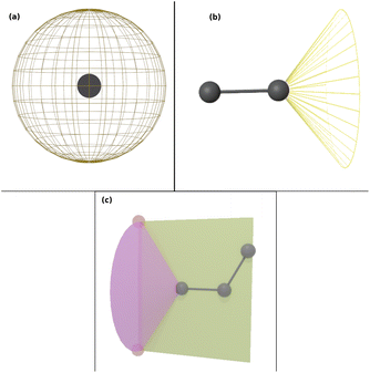 | ||
| Fig. 1 Possible places to put a new atom when (a) only one atom is present, (b) two atoms are present, and (c) three or more atoms are present (the red ghost atoms show the allowed positions). | ||
The energy change is calculated for each of these n positions. Finally, the ith configuration is selected from the Boltzmann distribution of these states based on the energy computed:
 | (1) |
 | (2) |
 | (3) |
2.1.2.3 Picking the next atom-type. At each step, SPOTLIGHT uses a rules-based system for choosing the next atom to pick. For example, a carbonyl carbon atom must connect to a carbonyl oxygen atom. Sometimes, multiple atoms are also allowed. For example, an aromatic carbon atom has to be part of a benzene-like ring, but the substituent (third neighbor outside the ring) can be anything. In this case, one is chosen randomly. Note that we will modify this choice of selection later when we introduce reinforcement learning in Section 2.2. This selection will eventually determine molecule-level properties.
2.1.2.4 Computing interaction energies. For every newly added atom, the energy with every atom in the protein is calculated. The energy functions used are LJ and coulombic interactions in accordance with the classical CHARMM force field, formulated as:
 | (4) |
 | (5) |
These parameters are additive over atom pairs (i.e., the energy between two molecules is the sum of the pairwise atom interaction energies), which is common for most classical force fields.31 This additivity makes atomistic generation efficient. We also emphasize that the CBMC-like approach we follow requires this property to ensure the accuracy of the Rosenbluth method in generating stable configurations of the molecule as ΔE (change in energy) is computed per atom, and its energy contribution should not change irrespective of the atoms added later on.
To improve the efficiency as most of the time is spent in this phase, we use a cut-off of 1 nm for LJ potential (as the interaction strength drops of significantly by this point), but a very long 5 nm cut-off for electrostatic interactions.
2.1.2.5 Recoil. An intermediate state during the generation phase is called a dead-end if placing the atom is necessary to satisfy the requirements of a particular atom-type, but it cannot be placed without having it clash (overlap of the van der Waals radii) with either the protein or the molecule itself. For example, this could be when a carbonyl carbon atom is placed, but any possible place to put the oxygen atom would clash with the protein. To avoid such dead-ends, the algorithm checkpoints the growth at every stage where the rules for every atom-type are satisfied (i.e., when all six atoms of a benzene ring or both the carbon and oxygen atoms in a carbonyl group have been placed).
On reaching a dead-end, the growth recoils to the nearest checkpoint. Every checkpoint has a certain number of trials (here, 15) allowed. If a certain number of recoil attempts fails, the entire fragment is abandoned, and generation is started afresh.
2.1.2.6 Traversing chemical space. As mentioned before, we utilize configurational bias-like position selection only to produce a stable 3D bound pose of the ligand with a low rejection rate. Reproducing the true distribution of binding molecules is not relevant to us. We want to traverse chemical space efficiently without cornering ourselves into the strongest molecule alone. Therefore, up to some variation, we prefer molecules with low binding energies; so we omit the reweighting part of the Rosenbluth sampling and look to Metropolis Monte-Carlo, as mentioned below, to traverse chemical space.
If we have two molecules (say A and B) with different binding energies (say ΔEA and ΔEB) competing for binding to the same target location, the probability of finding molecule A is proportional to exp(−ΔEA). The ratio of probabilities is given by:
 | (6) |
2.1.2.7 Temperature as a variability parameter. In some cases, optimization algorithms using Metropolis Monte-Carlo treat temperature as a tuning parameter to balance variety with optimization.32 Such an interpretation is possible with SPOTLIGHT as well. Increasing the temperature corresponds to larger oscillations in energy, resulting in less optimal but more varied molecules (useful when other key properties not captured by interaction strength are also necessary). Lowering the temperature reduces the variety and makes the algorithm slower but leads to better optimization. Sometimes, it may also lead to non-convergence due to higher rejection. A temperature range of 300 K–1200 K has been found to be quite reasonable and successful in previous use-cases.33
We acknowledge that this way of using biased sampling can also bias the configurations of molecules we make towards specific binding modes without adequately considering the space of all configurations. However, the goal here is to find molecules with stronger interaction and not so much to have a canonical ensemble of all possible binders in all possible binding poses.
2.1.2.8 Fine-tuning the selection. It is normal to have energy oscillations in Metropolis Monte-Carlo. Therefore, directly allowing extremely poor binders as part of the Metropolis scheme is unfavorable. To encourage variability without affecting the interaction scores, we also perform heuristic fine-tuning. Instead of allowing all the molecules, we take the average score of the last batch of molecules after every few oscillations (decided by the user). Then, we only pick the molecules with scores better than the average for that batch. We repeat this process until a desired number of final molecules is reached.
2.1.2.9 Additional options. The program allows users to restrain the molecule's growth to a specific region to ensure a more efficient search in the hotspot (the active site region). The program also allows the user to perform short optimizations to the molecule after the generation is complete. The final conformation is then obtained through gradient descent of the molecule in the presence of the protein.
2.2 Applying reinforcement learning
In this section, we are going to discuss how reinforcement learning (RL) is used to generate molecules that not only will bind strongly to the receptor but also will have the desired properties. Note that while atom-type rules have been hard-coded into the program, there is flexibility in the choice of atom-type at every stage in the growth of the molecule where a new atom is being added. We realized that any change in the choice of atom-type affects the kinds of molecules generated. In our approach discussed above, atom-types were chosen randomly as long as they conform to some objective rules. We modify that choice here using a reinforcement algorithm, where a machine-learned agent chooses the next atom-type to optimize the generation of molecules with specific molecule-level properties such as synthesizability, log![[thin space (1/6-em)]](https://www.rsc.org/images/entities/char_2009.gif) P values, drug-likeness, etc. The model is a Graph Convolution Policy Network (GCPN),34 simplified slightly to suit SPOTLIGHT.
P values, drug-likeness, etc. The model is a Graph Convolution Policy Network (GCPN),34 simplified slightly to suit SPOTLIGHT.
Classically, GCPN was also applied to molecule generation networks that string atoms together.34 It acts on a graph G as input with nodes representing the atoms and edges representing the bonds. The edges also explicitly have bond-order information. Starting from an arbitrary partially-formed molecule, it could perform one of two things at each step – add another atom to the molecule at a point where there is a free valency or join two atoms in the existing molecule (achieving cyclization).
We implement a slightly different version of classical GCPN. We represent an incomplete molecule by a graph G ≡ (V, E) where V ∈ ![[Doublestruck R]](https://www.rsc.org/images/entities/char_e175.gif) nxd contains the d features for each of the (maximum of n) atoms (nodes) and E ∈ {0,1}nxn is the adjacency matrix. We don't store bond order information since atom-types can be used to determine it. A key difference in our model is that we use a changing action space. Unlike traditional GCPN,34 SPOTLIGHT already picks the first atom (the focal atom) to which we will add our next atom. The action space for each state is the list of allowed atom-types (according to force field rules) to connect to the focal atom. The size of this list can vary. Once the model picks an atom-type, the positioning and cyclization are also taken care of by the traditional method, where we complete a cycle if the new atom falls within bonding distance of another atom with a free valency.
nxd contains the d features for each of the (maximum of n) atoms (nodes) and E ∈ {0,1}nxn is the adjacency matrix. We don't store bond order information since atom-types can be used to determine it. A key difference in our model is that we use a changing action space. Unlike traditional GCPN,34 SPOTLIGHT already picks the first atom (the focal atom) to which we will add our next atom. The action space for each state is the list of allowed atom-types (according to force field rules) to connect to the focal atom. The size of this list can vary. Once the model picks an atom-type, the positioning and cyclization are also taken care of by the traditional method, where we complete a cycle if the new atom falls within bonding distance of another atom with a free valency.
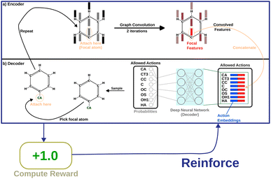
Message-passing35 combines information from neighboring nodes to enrich the information in each node. Iterative message passing can also be used to incorporate information from farther nodes. In this work, we show the use of graph convolution36 in encoding neighbourhood information into the focal atom. This part of the model is called the “encoder”. The encoded information is then utilized by a simple, fully connected layer (the “decoder”) to produce probabilities as output. Fig. 2 shows how the model is set up.
The first step is encoding the molecule. We use one-hot encoding37 as node features for the atoms. For one-hot encoding, the list of all atom-types is placed in an ordered list. To convert an atom of type “T” to its corresponding vector, we construct the vector representation as follows:
| One-hot (T): = (1T(i); i ∈ 1.166) | (7) |
| 1T(i): = 1 if T is the ith atom-type, else 0 | (8) |
For the adjacency matrix, we use a simple matrix, A, of 0's and 1's to denote bonds:
| Aij: = 1, if atoms i and j are bonded; 0 otherwise | (9) |
The next step is the implementation of the graph convolution. In this work, we have used two iterations of graph convolution with the input and output dimension of 166. The convolved feature vector for each node (atom) is obtained. However, only the one for the focal atom is considered for deciding the action. Based on atom-type rules, SPOTLIGHT provides a list of atom-types that are “allowed” neighbors for a given focal atom. We take the encoding for each allowed atom-type (in our case, one-hot encoding) and concatenate the convolved focal atom feature vector to these vectors. This concatenation combines the information about the newly added atom-type and the current state of the focal atom, forming a set of k encoded vectors where k is the number of allowed atom-types at this stage. This dependence of k on the number of allowed neighbors makes the number of legal actions variable depending on the current state. To account for this, our model deals with varying-sized valid action spaces.
Finally, each vector is passed through a two-layer, fully connected network (decoder in Fig. 2). The first layer has 128 neurons, and the second (output layer) has only one. A ReLu activation function is used after the first layer. After the second layer, every encoded vector now gets a single number as output. We take the value for each and use the softmax function to convert the list of values into probabilities – commonly used to model policies in RL.38
 | (10) |
The policy yields probabilities for each “allowed” atom-type. One atom-type is picked from the list; thus, the (growing) molecule's size increases by one atom. This process is repeated until the target size is reached or all valencies are filled. Fig. S3 of the ESI† elaborates on the model scheme.
The model is trained through back-propagation, using the Adam39 optimizer with a learning rate of 9.5 × 10⁻⁴ and default parameters using PyTorch.40 The training was done in multiple cycles of optimizing the same model while tuning the learning rate. This process is explained while discussing the results. The model is trained through RL using the classic REINFORCE41 algorithm. Following the standard protocol, a small negative reward of −0.01 is given for each step, and a positive reward of +1 is given if the final molecule (once it reaches the target size) is synthesizable and −1 if not. A heavy penalty of −7.5 is levied if the model fails to reach the target size, which usually happens if all valences are filled before the required size is reached.
Reinforcement learning models are not typically implemented with a varying number of actions depending on the state. However, our models work well with varying actions. Therefore, this setup might be helpful in building models for similar use cases. We later present our results with synthesizability as determined by the SYBA42 classifier. In principle, any scoring function would work here, but it requires significant training time and tuning of the model's hyperparameters.
2.3 Parameterization in Gaussian
Force field charges for some newly added atom types need to be computed afresh. Gaussian 09 was used to compute the partial charges for these cases. Minimal molecules containing the atom type were chosen to be chargeless (unless a particular atom-type itself was charged). They were all optimized at the HF/6-31G* level of theory, and the ESP fit was obtained. Antechamber43 was used to check the structural integrity of the fragments and to handle the file format conversion from PDB to a Gaussian input format. Finally, the Gaussian output was converted to mol2 format,44 which contains charges. To bring these charges in line with the charges already present in CHARMM, the charges were scaled by a factor of 0.87, obtained by taking the ratio of ESP charges to CHARMM charges in a benzene molecule. These values were not changed if charges were already available.2.4 Using the SYBA model
The SYBA model is a naïve Bayes model that classifies every ligand as ES (easy-to-synthesize) or HS (hard-to-synthesize). It assigns scores to many molecular fragments and combines them to yield the log odds for a molecule to be synthesizable. SYBA is trained on the ZINC15 database of molecules, which are assumed to be synthesizable. It uses Nonpher,45 a software that iteratively makes simple structural changes to a given molecule, to artificially create examples of hard-to-synthesize molecules starting from these molecules. It is shown to yield molecules that are not overly complex on paper, but are hard to synthesize.45 SYBA was then trained to classify molecules based on these two sets of positive and negative examples.3 Results and discussion
SPOTLIGHT is a computational drug design algorithm capable of atomistically generating a variety of novel synthesizable molecules that are likely potent inhibitors for a given target. We present our results to show that it can satisfy multiple goals simultaneously.3.1 Training by RL for synthesizability
SPOTLIGHT can make a sample of molecules even when no receptor is provided. To train our RL algorithm for generating molecules with desired properties, the molecules are first made in the vacuum, with the only energy terms coming from the self-energy. Since there is no Metropolis Monte-Carlo rejection (because there is no protein–ligand interaction energy), every completed molecule is accepted. A generation like this allows us to study the algorithm's properties without having protein scaffolds that could interfere with the generation by providing biases for some molecules to be more viable.We now check a rather important parameter for generative models – variation.46 For an algorithm like SPOTLIGHT that does not parallelly optimize too many properties of the molecules, a reasonable variation among the molecules is helpful as it allows at least some molecules to have multiple favorable properties other than just strong protein binding.
We use the self-similarity distribution (SSD) as a measure of variability. The SSD is the distribution of self-similarity (SS) of a set of size N, defined as follows.
| SS: = {maxj≠i{sim(mi,mj); 0 ≤ j ≤ N}; 0 ≤ i ≤ N} | (11) |
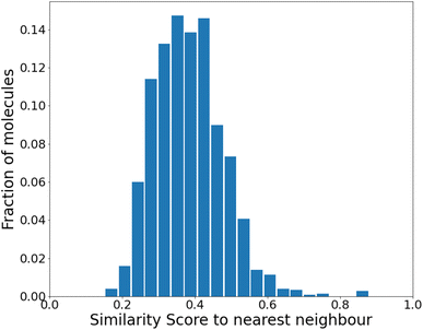 | ||
| Fig. 3 Similarity to the nearest neighbor in the same set before any reinforcement. The mean similarity is 0.39 ± 0.004. | ||
We find that the distribution peaks at a low similarity score of 0.39. Even when recomputed with 12![[thin space (1/6-em)]](https://www.rsc.org/images/entities/char_2009.gif) 000 molecules, it peaks below 0.6, with no significant peak at 1.0. This plot is shown in Fig. S4 of the ESI.† Compared to a previous method that dealt with generating varied molecules,41 this distribution implies substantial variation in our molecules. However, at this stage (before any training), only 24% of the molecules were found to be synthesizable as classified by SYBA.42
000 molecules, it peaks below 0.6, with no significant peak at 1.0. This plot is shown in Fig. S4 of the ESI.† Compared to a previous method that dealt with generating varied molecules,41 this distribution implies substantial variation in our molecules. However, at this stage (before any training), only 24% of the molecules were found to be synthesizable as classified by SYBA.42
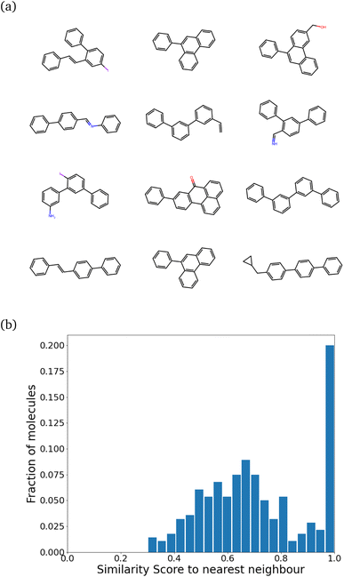
While training our model, we quickly realized that the model learns to pick up some key features of a molecule that make it synthesizable. Then, it repeats those features multiple times, making every molecule a tiled combination of similar atom-types, essentially losing out on the variance. Fig. 4a shows how similar the molecules can get. Fig. 4b shows the SSD for these molecules.
The program begins to string together aromatic rings at different points. It likely picks up on the importance of aromatic atom-types in easily achieving simple molecules (most benzene derivatives are synthesizable). This blind emphasis on aromaticity is useless as it forces the program to collapse to search in an extremely narrow region of the chemical space. However, the model achieves the task very well. Almost 99% of molecules are synthesizable – a stunningly high amount.
The peak at the similarity score of 1.0 is indicative of a mode collapse. Mode collapse is a problem seen with generative models where they learn a solution that technically does minimize the loss but miss “modes”, resulting in the generation of a very narrow band of results from the complete space available to them.49 In our case, we only obtain molecules with aromatic rings strung together. This is not very useful, and we needed to regularize it. The word “regularize” is used here as a parallel to the regularization in polynomial fitting, where the model's quality is traded for a more useful model that can be extrapolated more reliably (bias–variance trade-off). In our case, regularization allows the model to sacrifice some synthesizability to generate a more diverse range of molecules. We observed that one requires, heuristically, the peak to stay below 0.55 for 300 molecules with no significant peak at 1.0 to get a diverse set of molecules.
For regularization, we used a proxy for Tanimoto similarity, called cosine similarity of a vector representation of each molecule (denoted cosim), during training to speed up training time. As mentioned above, each molecule was represented by a 166-dimensional feature vector – with each index corresponding to one atom-type. The value at each index conveys what fraction of atoms in the molecule had that particular atom-type. For example, benzene would have values of 0.5 for “aromatic carbon” and 0.5 for “aromatic-attached hydrogen” indices, and 0 elsewhere. We then applied a measure of variance as a regularization term to the final reward for the ith molecule when it was synthesizable. This changes the reward scheme as follows:
 | (12) |
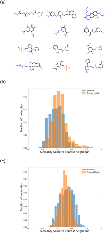
We then retrained the model with different values of λ, increasing it until the SSD for the molecules after training was acceptable (low mean similarity of 0.43). Fig. 5 shows how the similarity changes after training.
We found that keeping λ fixed throughout the training was inefficient. Starting with a very high value of λ did not allow the model to learn quickly. Instead, we trained it with λ = 1.60 for around 7500 molecules, saving the model after every 50 iterations. We picked the model after 3500 molecules (chosen to have an optimal increase in synthesizability with minimal change in SSD) and followed it by around 4200–4500 molecules each for λ = 2.00, λ = 2.35 and finally λ = 2.60. Each molecule generated can be considered to be one “episode”. The evolution of the reward profile with changing values of λ is given in Fig. S5 of the ESI.† After training with this method, about 78.2% of the molecules turned out to be synthesizable, which is a big improvement over the 24% we had without training. The main computational cost for this setup is actually the energy computation step for each trial atom placement, and the RL part (especially during inference) takes very little time. A model that can learn efficiently, with only a few molecules generated, would be ideal. Under this setup of training, the 7500 molecules involved in training are generated in less than 24 hours on an Intel i7-8700 processor running on 6 cores (12 threads in total).
For all these plots, the chosen target size of the molecule (in heavy atoms) for each generation was 21 ± 5, which is roughly near the most populous region of the CheMBL database – on the lower end. The choice of training and test size ranges, as reflected in the CheMBL molecules' size distribution, is shown in Fig. S6 of the ESI.† We trained on smaller sizes to ensure quick training and efficient detection of generative mode-collapse by monitoring the Tanimoto similarity score. A similar analysis is performed for generating molecules of a larger size (see Fig. 5c) to ensure good performance of the model even on increasing molecule size beyond the training range. The effect of regularization is more prominent at larger sizes, reducing the mean similarity to the nearest neighbor from 0.53 for the baseline to 0.51 after training.
We also saw that the similarity distributions shift to the right with increasing size, which probably indicates that larger molecules tend to have more fragments in common with each other. However, the probability of finding multiple similar fragments on the same molecule decreases, which could explain the greater influence of regularization at higher target sizes.
3.2 Characteristics of the generated molecules
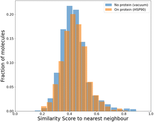
While we have used generic atom-types, there could be some intrinsic bias towards known molecules by choice of rules made to ensure proper cyclization and chemical viability.Fig. 6 shows the distribution of the similarity of our molecules to the existing CheMBL50 database. We find a low mean similarity of 0.42, which increases to 0.52 after training. Most molecules have a similarity below 0.6, which means these are indeed novel molecules. The program can thus pick up ways of making synthesizable molecules without reproducing preexisting molecules. This novelty was expected given that the program has no information from CheMBL fed to it at any point, but it is worthwhile to note that no significant bias creeps in by using the SYBA model as a classifier for synthesizability. In all cases, almost no molecules have a similarity above 0.8.
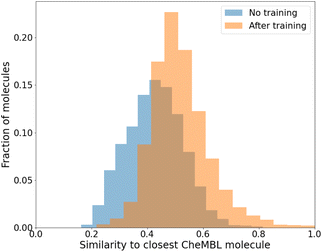 | ||
Fig. 6 Similarity of generated molecules with the closest match from the CheMBL database. The sample size was 12![[thin space (1/6-em)]](https://www.rsc.org/images/entities/char_2009.gif) 000 molecules of sizes roughly between 16 and 26 heavy atoms. 000 molecules of sizes roughly between 16 and 26 heavy atoms. | ||
To compare how the model performs to other metrics, we compared the molecules generated before training and after training by their QED51 (an estimation of drug-likeness) scores. The mean shifts from 0.34 ± 0.2 to 0.44 ± 0.22. 39% of the molecules have a score above 0.5 after training, compared to only 22% before. A similar QED distribution of the CheMBL molecules we used has a median of 0.56. Only 16.6% of the molecules could achieve this rating before training, which almost doubles to 31% after. The complete distribution is shown in Fig. S7 of the ESI.†
3.3 Upscaling
The model has been trained and tested for molecules with sizes (heavy atom count) between 16 and 26. We considered the effect of using the same model for larger sizes and found promising results even when we targeted sizes in the range 36 ± 5 with the same model. Fig. 5c shows almost no difference in the SSD between the baseline (no training) and the trained model, implying no loss in diversity. In fact, the similarity between molecules is reduced, indicating the effectiveness of regularization. However, the synthesizable fraction improves significantly from 8.3% to over 70%. Fig. S8 of the ESI† shows the synthesizability as a function of heavy-atom count before and after training.3.4 Effect of GCN layers on SSD scores and synthesizability
We ideally want to have as low an SSD score as possible and as high a synthesizability fraction as possible. The following table summarizes our results with different models at a target size of 21 ± 5 (“reg.” denotes the use of regularization during training). The errors were calculated based on five replicate runs of each case, except for the unregularized one-layer GCN model (Table 1).We find that using two layers made the model slightly more competent and strategies learnt by the 2 layer models are more robust, resulting in a quicker satisfaction of atom-type rules and over 2× decrease in runtime for molecule generation overall. We also noticed that it generalized better to larger sizes (data provided in Fig. S9 of the ESI†), so further analyses are performed with a model that uses two iterations of graph convolution.
3.5 Application to HSP90
To compare our protocol to a system with known binders, we targeted the ATP binding site of HSP90 (heat-shock protein 90), known for the folding of other proteins in a cell.52 HSP90, with its extremely well-conserved ATP-binding domain, is an important therapeutic target and has been targeted for cancer treatment.53We targeted this ATP binding site using SPOTLIGHT. Because there are known ligands for this protein,54 it is a good benchmark system having a well-established 3D crystal structure of the active site. The crystal structure of HSP90 was obtained from the protein data bank (PDB) with PDB ID 2VCI. All ligands and water molecules were removed from the PDB file, and the protein structure was provided to SPOTLIGHT. We marked the ATP binding region to be the active site (residues Leu33, Asn36, Ser37, Asp39, Ala40, Lys43, Asp78, Gly80, Ile81, Gly82, Met83, Thr84, Asp87, Leu92, Gly93, Thr94, Ile95, Gly120, Phe123, Val135, Thr137, His139, Thr169, and Val171). To create molecules that are varied, synthesizable, and strong binders to the HSP90 protein, we generated around 800 molecules each for all sizes between 16 to 26 heavy atoms.
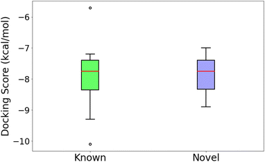
An independent docking analysis using AutoDock Vina56 also shows that SPOTLIGHT is capable of predicting lead molecules with binding strength comparable to some of the best-known binders for HSP90. Fig. 11 shows a box plot comparing the docking scores of the 28 best-known binders to the top 25 molecules as predicted by SPOTLIGHT's interaction energy. Known ligands within the target size range of 22–32 are selected here, accounting for 28 of the 50. The target size for the SPOTLIGHT generations is the same, given that ligand size itself (or rather torsion count, which scales with size) can affect docking scores.57 The final size distribution for the known ligands was 27.0 ± 2.56 and 27.3 ± 2.55 for our top ligands.
4 Conclusions and further discussion
SPOTLIGHT is a powerful program capable of producing a variety of competent and synthesizable drug molecules for a given protein target. The sampling process is efficient as it generates molecules directly in the active site. SPOTLIGHT provides effective lead candidates. However, further modifications are required to turn the most attractive candidates into clinically viable drug molecules.The algorithm is extremely modular. This study is a proof-of-concept of its capabilities. Many components in the problem of computer-aided drug design (CADD) can be independently optimized. The algorithm provides scope to allow necessary changes to be incorporated in light of important future developments. The reinforcement model we use is a simple graph convolution network. However, more complex models, such as attention networks,58 could be used for greater success with enough training time and a potentially better-formulated reward function. We found that other models that use only composition data could not abstract out molecule synthesizability, while the simple graph representation was successful at the same task. However, it might be useful to look at different methods of encoding for other properties. On another front, we address mode-collapse by using a manual regularization. However, our regularization scheme needs fine tuning of the hyper-parameter (λ) to achieve required thresholds. Other methods have been recently developed to combat mode collapse, such as the ones used in REINVENT4, which avoids the λ parameter entirely, which might prove useful if the objective function is changed in the future.
The program allows for a secondary scoring function to weigh in on the quality of a molecule. If the user prefers to use their own scoring (such as docking), the option to do so is provided. However, it would require source code changes. Improving the current scoring function is important. The protein is rigid during the generation. To incorporate flexibility in the protein, one can pre-generate the conformation by sampling the protein through simulations and clustering different conformations. The program still can't account for the effects of water. Although the dielectric constant is used to take the screening effect into account for energetic components, water entropy contribution to the free energy can't be incorporated readily yet. Improved energy functions, maybe with machine-learned force fields, could be used to improve the interaction energy between the ligand and protein.
SPOTLIGHT is a promising method, but it will be useful to compare it to other methods that independently generate their ligands and then use docking cycles for training to generate strong binders. However, an independent and more rigorous method of comparing binding constants (such as metadynamics) will be required for this analysis, which is computationally quite expensive to perform for as many ligands.
We intend to address these drawbacks in our future work.
Data availability
The code for SPOTLIGHT, developed by us and as described in this article, is available at https://github.com/arnabpune/SPOTLIGHT. The SMILES generated in the analyses described here (and a brief description) are available in a zip file named SMILES_data.zip. This study was carried out using publicly available data from CheMBL's small-molecule dataset accessible at https://www.ebi.ac.uk/chembl/. A collated list of molecules with ∼7–61 heavy atoms is present in the above-mentioned zip file. The SYBA tool used to classify molecules to be synthesizable was installed using conda, following the instructions from the relevant git repository: https://github.com/lich-uct/syba. The RDKit (version 2019.03) package was mainly used for handling molecule-level analyses. This release is available at: https://github.com/rdkit/rdkit/releases/tag/Release_2019_09_3.Author contributions
The manuscript was written through the contributions of all authors.Conflicts of interest
There are no conflicts to declare.Acknowledgements
We acknowledge PARAM Brahma under the National Supercomputing Mission (NSM), Government of India, for providing computational facilities for this work. We thank DBT, Govt. of India (Grant no. BT/PR34215/AI/133/22/2019) for partial funding.References
- P. G. Polishchuk, T. I. Madzhidov and A. Varnek, Estimation of the size of drug-like chemical space based on GDB-17 data, J. Comput.-Aided Mol. Des., 2013, 27, 675–679 CrossRef CAS PubMed.
- G. Sliwoski, S. Kothiwale, J. Meiler and E. W. L. Jr, Computational Methods in Drug Discovery, Pharmacol. Rev., 2014, 66, 334–395 CrossRef PubMed.
- S. B. Mirza, R. E. Salmas, M. Q. Fatmi and S. Durdagi, Virtual screening of eighteen million compounds against dengue virus: Combined molecular docking and molecular dynamics simulations study, J. Mol. Graphics Modell., 2016, 66, 99–107 CrossRef CAS PubMed.
- W. Walters, M. T. Stahl and M. A. Murcko, Virtual screening—an overview, Drug Discovery Today, 1998, 3, 160–178 CrossRef CAS.
- A. C. Anderson, The Process of Structure-Based Drug Design, Chem. Biol., 2003, 10, 787–797 CrossRef CAS PubMed.
- H. Berman, J. Westbrook, Z. Feng, G. Gilliland, T. Bhat, H. Weissig, I. Shindyalov and P. Bourne, The Protein Data Bank, Nucleic Acids Res., 2000, 28, 235–242 CrossRef CAS PubMed.
- N. Coleman and J. Rodon, Taking Aim at the Undruggable, American Society of Clinical Oncology Educational Book, 2021, pp. e145–e152 Search PubMed.
- M. L. Cohen, Epidemiology of Drug Resistance: Implications for a Post—Antimicrobial Era, Science, 1992, 257, 1050–1055 CrossRef CAS PubMed.
- B. Jayaram, T. Singh, G. Mukherjee, A. Mathur, S. Shekhar and V. Shekhar, Sanjeevini: a freely accessible web-server for target directed lead molecule discovery, BMC Bioinf., 2012, 13, S7 CrossRef PubMed.
- R. Wang, Y. Gao and L. Lai, LigBuilder: A Multi-Purpose Program for Structure-Based Drug Design, J. Mol. Model., 2000, 6, 498–516 CrossRef CAS.
- F. Chevillard, H. Rimmer, C. Betti, E. Pardon, S. Ballet, N. van Hilten, J. Steyaert, W. E. Diederich and P. Kolb, Binding-Site Compatible Fragment Growing Applied to the Design of β2-Adrenergic Receptor Ligands, J. Med. Chem., 2018, 61, 1118–1129 CrossRef CAS PubMed.
- H.-J. Böhm, The computer program LUDI: A new method for the de novo design of enzyme inhibitors, J. Comput.-Aided Mol. Des., 1992, 6, 61–78 CrossRef PubMed.
- C. Lu, S. Liu, W. Shi, J. Yu, Z. Zhou, X. Zhang, X. Lu, F. Cai, N. Xia and Y. Wang, Systemic evolutionary chemical space exploration for drug discovery, J. Cheminf., 2022, 14, 19 CAS.
- V. D. Mouchlis, A. Afantitis, A. Serra, M. Fratello, A. G. Papadiamantis, V. Aidinis, I. Lynch, D. Greco and G. Melagraki, Advances in De Novo Drug Design: From Conventional to Machine Learning Methods, Int. J. Mol. Sci., 2021, 22, 1676 CrossRef PubMed.
- Y. Nishibata and A. Itai, Automatic creation of drug candidate structures based on receptor structure. Starting point for artificial lead generation, Tetrahedron, 1991, 47, 8985–8990 CrossRef CAS.
- J. O. Spiegel and J. D. Durrant, AutoGrow4: an open-source genetic algorithm for de novo drug design and lead optimization, J. Cheminf., 2020, 12, 25 CAS.
- M. Popova, O. Isayev and A. Tropsha, Deep reinforcement learning for de novo drug design, Sci. Adv., 2018, 4–7 Search PubMed.
- M. Goel, S. Raghunathan, S. Laghuvarapu and U. D. Priyakumar, MoleGuLAR: Molecule Generation Using Reinforcement Learning with Alternating Rewards, J. Chem. Inf. Model., 2021, 61, 5815–5826 CrossRef CAS PubMed.
- Y. Kwon and J. Lee, MolFinder: an evolutionary algorithm for the global optimization of molecular properties and the extensive exploration of chemical space using SMILES, J. Cheminf., 2021, 13, 24 CAS.
- H. Loeffler, J. He, A. Tibo, J. P. Janet, A. Voronov, L. Mervin and O. Engkvist, REINVENT4: Modern AI-Driven Generative Molecule Design, ChemRxiv, 2023, preprint, DOI:10.26434/chemrxiv-2023-xt65x.
- M. Šícho, S. Luukkonen, H. W. van den Maagdenberg, L. Schoenmaker, O. J. M. Béquignon and G. J. P. van Westen, DrugEx: Deep Learning Models and Tools for Exploration of Drug-Like Chemical Space, J. Chem. Inf. Model., 2023, 63, 3629–3636 CrossRef PubMed.
- M. N. Rosenbluth and A. W. Rosenbluth, Monte Carlo Calculation of the Average Extension of Molecular Chains, J. Chem. Phys., 1955, 23, 356–359 CrossRef CAS.
- J. I. Siepmann and D. Frenkel, Configurational bias Monte Carlo: a new sampling scheme for flexible chains, J. Mol. Phys., 1992, 75, 59–70 CrossRef CAS.
- H. A. Zhong, in ADMET Properties: Overview and Current Topics, Springer, Singapore, 2017, pp. 113–133 Search PubMed.
- A. D. Mackerell Jr, M. Feig and C. L. Brooks 3rd, Extending the treatment of backbone energetics in protein force fields: limitations of gas-phase quantum mechanics in reproducing protein conformational distributions in molecular dynamics simulations, J. Comput. Chem., 2004, 25(11), 1400–1415 CrossRef PubMed.
- M. J. Frisch, G. W. Trucks, H. B. Schlegel, G. E. Scuseria, M. A. Robb, J. R. Cheeseman, G. Scalmani, V. Barone, G. A. Petersson, H. Nakatsuji, X. Li, M. Caricato, A. Marenich, J. Bloino, B. G. Janesko, R. Gomperts, B. Mennucci, H. P. Hratchian, J. V. Ortiz, A. F. Izmaylov, J. L. Sonnenberg, D. Williams-Young, F. Ding, F. Lipparini, F. Egidi, J. Goings, B. Peng, A. Petrone, T. Henderson, D. Ranasinghe, V. G. Zakrzewski, J. Gao, N. Rega, G. Zheng, W. Liang, M. Hada, M. Ehara, K. Toyota, R. Fukuda, J. Hasegawa, M. Ishida, T. Nakajima, Y. Honda, O. Kitao, H. Nakai, T. Vreven, K. Throssell, J. A. Montgomery Jr, J. E. Peralta, F. Ogliaro, M. Bearpark, J. J. Heyd, E. Brothers, K. N. Kudin, V. N. Staroverov, T. Keith, R. Kobayashi, J. Normand, K. Raghavachari, A. Rendell, J. C. Burant, S. S. Iyengar, J. Tomasi, M. Cossi, J. M. Millam, M. Klene, C. Adamo, R. Cammi, J. W. Ochterski, R. L. Martin, K. Morokuma, O. Farkas, J. B. Foresman and D. J. Fox, Gaussian 09, Revision D.01, 2009 Search PubMed.
- D. V. D. Spoel, E. Lindahl, B. Hess, G. Groenhof, A. E. Mark and H. J. C. Berendsen, GROMACS: Fast, flexible, and free, J. Comp. Chem, 2005, 26, 1701–1718 CrossRef PubMed.
- M. Abraham, D. van der Spoel, E. Lindahl, B. Hess and T. G. development team, GROMACS version 2018, 2018 Search PubMed.
- D. Frenkel, G. C. A. M. Mooij and B. Smit, Novel scheme to study structural and thermal properties of continuously deformable molecules, J. Phys.: Condens. Matter, 1992, 4, 3053 CrossRef.
- N. Metropolis, A. W. Rosenbluth, M. N. Rosenbluth, A. H. Teller and E. Teller, Equation of State Calculations by Fast Computing Machines, J. Chem. Phys., 1953, 21, 1087–1092 CrossRef CAS.
- L. Monticelli and D. P. Tieleman, in Ch. 8: Force Fields for Classical Molecular Dynamics, Humana Press, 2013, pp. 197–213 Search PubMed.
- Z. Li and H. A. Scheraga, Monte Carlo-minimization approach to the multiple-minima problem in protein folding, Proc. Natl. Acad. Sci. U. S. A., 1987, 84, 6611–6615 CrossRef CAS PubMed.
- R. Chowdhury, V. S. S. Adury, A. Vijay, R. K. Singh and A. Mukherjee, Atomistic De-novo Inhibitor Generation-Guided Drug Repurposing for SARS-CoV-2 Spike Protein with Free-Energy Validation by Well-Tempered Metadynamics, Chem.–Asian J., 2021, 16(12), 1634–1642 CrossRef CAS PubMed.
- J. You, B. Liu, R. Ying, V. Pande and J. Leskovec, Graph Convolutional Policy Network for Goal-Directed Molecular Graph Generation, arXiv, 2018, preprint, arXiv:1806.02473, DOI:10.48550/arXiv.1806.02473.
- J. Gilmer, S. S. Schoenholz, P. F. Riley, O. Vinyals and G. E. Dahl, in Message Passing Neural Networks, Springer International Publishing, Cham, 2020, pp. 199–214 Search PubMed.
- T. N. Kipf and M. Welling, Semi-Supervised Classification with Graph Convolutional Networks, arXiv, 2016, preprint, arXiv:1609.02907, DOI:10.48550/arXiv.1609.02907.
- P. Joshi, Python Machine Learning Cookbook, Packt Publishing Ltd, 2016, ch. 4 Search PubMed.
- B. Gao and L. Pavel, On the Properties of the Softmax Function with Application in Game Theory and Reinforcement Learning, arXiv, 2017, preprint, arXiv:1704.00805, DOI:10.48550/arXiv.1704.00805.
- D. P. Kingma and J. Ba: A Method for Stochastic Optimization, arXiv, 2014, preprint, arXiv:1412.6980, DOI:10.48550/arXiv.1412.6980.
- A. Paszke, S. Gross, F. Massa, A. Lerer, J. Bradbury, G. Chanan, T. Killeen, Z. Lin, N. Gimelshein, L. Antiga, A. Desmaison, A. Kopf, E. Yang, Z. DeVito, M. Raison, A. Tejani, S. Chilamkurthy, B. Steiner, L. Fang, J. Bai and S. Chintala, PyTorch: An Imperative Style, High-Performance Deep Learning Library, arXiv, 2019, preprint, arXiv:1912.01703, DOI:10.48550/arXiv.1912.01703.
- R. J. Williams, Simple statistical gradient-following algorithms for connectionist reinforcement learning, Mach Learn, 1992 Search PubMed.
- M. Voršilák, M. Kolář, I. Čmelo and D. Svozil, SYBA: Bayesian estimation of synthetic accessibility of organic compounds, J. Cheminf., 2020, 12, 35 Search PubMed.
- J. M. Wang, W. Wang, P. A. Kollman and D. A. Case, Automatic atom type and bond type perception in molecular mechanical calculations, J. Mol. Graphics Modell., 2006, 25, 247–260 CrossRef CAS PubMed.
- Tripos MOL2 Format, https://zhanggroup.org/DockRMSD/mol2.pdf, 2005.
- M. Voršilák and D. Svozil, Nonpher: computational method for design of hard-to-synthesize structures, J. Cheminf., 2017, 9, 20 Search PubMed.
- N. Brown, M. Fiscato, M. H. Segler and A. C. Vaucher, GuacaMol: Benchmarking Models for de Novo Molecular Design, J. Chem. Inf. Model., 2019, 59, 1096–1108 CrossRef CAS PubMed.
- P. Jaccard, author, Bull. Soc. Vaudoise Sci. Nat., 1901, 37, 547–589 Search PubMed.
- G. Landrum, RDKit: Open-Source Cheminformatics Software, 2016 Search PubMed.
- B. V. Kushwaha and G. C. Nandi, 2020 IEEE 4th Conference on Information & Communication Technology (CICT), 2020 Search PubMed.
- A. Gaulton, L. J. Bellis, A. P. Bento, J. Chambers, M. Davies, A. Hersey, Y. Light, S. McGlinchey, D. Michalovich, B. Al-Lazikani and J. P. Overington, ChEMBL: a large-scale bioactivity database for drug discovery, Nucleic Acids Res., 2011, 40, D1100–D1107 CrossRef PubMed.
- G. R. Bickerton, G. V. Paolini, J. Besnard, S. Muresan and A. L. Hopkins, Quantifying the chemical beauty of drugs, Nat. Chem., 2012, 4, 90–98 CrossRef CAS PubMed.
- S. E. Jackson, in Hsp90: Structure and Function, ed. S. Jackson, Springer Berlin Heidelberg, 2013, pp. 155–240 Search PubMed.
- M. Goetz, D. Toft, M. Ames and C. Erlichman, The Hsp90 chaperone complex as a novel target for cancer therapy, Ann. Oncol., 2003, 14, 1169–1176 CrossRef CAS PubMed.
- P. A. Brough, W. Aherne, X. Barril, J. Borgognoni, K. Boxall, J. E. Cansfield, K.-M. J. Cheung, I. Collins, N. G. M. Davies, M. J. Drysdale, B. Dymock, S. A. Eccles, H. Finch, A. Fink, A. Hayes, R. Howes, R. E. Hubbard, K. James, A. M. Jordan, A. Lockie, V. Martins, A. Massey, T. P. Matthews, E. McDonald, C. J. Northfield, L. H. Pearl, C. Prodromou, S. Ray, F. I. Raynaud, S. D. Roughley, S. Y. Sharp, A. Surgenor, D. L. Walmsley, P. Webb, M. Wood, P. Workman and L. Wright, 4,5-Diarylisoxazole Hsp90 Chaperone Inhibitors: Potential Therapeutic Agents for the Treatment of Cancer, J. Med. Chem., 2008, 51, 196–218 CrossRef CAS PubMed.
- T. Liu, Y. Lin, X. Wen, R. N. Jorissen and M. K. Gilson, BindingDB: a web-accessible database of experimentally determined protein–ligand binding affinities, Nucleic Acids Res., 2006, 35, D198–D201 CrossRef PubMed.
- O. Trott and A. J. Olson, AutoDock Vina: improving the speed and accuracy of docking with a new scoring function, efficient optimization, and multithreading, J. Comput. Chem., 2010, 31, 455–461 CrossRef CAS PubMed.
- D. K. Sriramulu, S. Wu and S.-G. Lee, Effect of ligand torsion number on the AutoDock mediated prediction of protein-ligand binding affinity, J. Ind. Eng. Chem., 2020, 83, 359–365 CrossRef CAS.
- P. Velisčković, G. Cucurull, A. Casanova, A. Romero, P. Liò and Y. Bengio, Graph Attention Networks, arXiv, 2018, preprint, arXiv:1710.10903, DOI:10.48550/arXiv.1710.10903.
Footnote |
| † Electronic supplementary information (ESI) available. See DOI: https://doi.org/10.1039/d3dd00194f |
| This journal is © The Royal Society of Chemistry 2024 |

