Active learning of neural network potentials for rare events

Abstract

Atomistic simulation with machine learning-based potentials (MLPs) is an emerging tool for understanding materials' properties and behaviors and predicting novel materials. Neural network potentials (NNPs) are outstanding in this field as they have shown a comparable accuracy to ab initio electronic structure calculations for reproducing potential energy surfaces while being several orders of magnitude faster. However, such NNPs can perform poorly outside their training domain and often fail catastrophically in predicting rare events in molecular dynamics (MD) simulations. The rare events in atomistic modeling typically include chemical bond breaking/formation, phase transitions, and materials failure, which are critical for new materials design, synthesis, and manufacturing processes. In this study, we develop an automated active learning (AL) capability by combining NNPs and one of the enhanced sampling methods, steered molecular dynamics, for capturing bond-breaking events of alkane chains to derive NNPs for targeted applications. We develop a decision engine based on configurational similarity and uncertainty quantification (UQ), using data augmentation for effective AL loops to distinguish the informative data from enhanced sampled configurations, showing that the generated data set achieves an activation energy error of less than 1 kcal mol⁻¹. Furthermore, we have devised a strategy to alleviate training uncertainty within AL iterations through a carefully constructed data selection process that leverages an ensemble approach. Our study provides essential insight into the relationship between data and the performance of NNP for the rare event of bond breaking under mechanical loading. It highlights strategies for developing NNPs of broader materials and applications through active learning.

---

1. Introduction

As the name implies, rare events are observed very infrequently. Pandemics, tornados, and stock market crashes are rare events in our daily lives. Although these events occur rarely, they can have long-lasting and catastrophic consequences. In atomistic modeling for materials science, rare events include chemical reactions, protein folding, and phase transitions. Another example of rare events is a material failure, a large deformation causing the material's structure to change shape or completely break apart. Such failure events can have catastrophic consequences, preventing materials from performing their intended roles, but they are also essential processes for fabricating materials. While studying rare events in materials systems is crucial, it is often challenging through conventional quantum/static approaches due to the time- and length scales that atomistic models can achieve. Therefore, predicting or simulating such behaviors in materials requires enhanced sampling techniques to capture these rare events appropriately. Such as energy barrier or activation energy for chemical bond breaking/formation and materials strength, are essential to understanding the materials' behaviors and deriving design principles for novel materials.

Computational modeling at the atomic scale approaches has been widely utilized to capture and understand these rare events. However, highly accurate quantum mechanics-based electronic structure approaches such as density functional theory (DFT) are computationally demanding and generally impractical for complex and large systems simulations over a long timescale. On the other hand, classical molecular mechanics-based forcefields, including reactive forcefields, can be used with larger systems, but their accuracy and transferability often need to be improved in specific applications.

Machine learning (ML) techniques have revolutionized problem-solving approaches in a wide range of fields of science and engineering.^1–6 Recent advances in physics-based computational atomistic modeling and simulations, in combination with artificial intelligence (AI) techniques, provide a novel avenue for materials design and efficient computational modeling.^7,8 In particular, recently developed ML-based potentials (MLPs)^9–11 has demonstrated a capability to predict potential energy surfaces (PESs) for atomic configurations with an accuracy comparable to ab initio electronic structure methods, but at a speed that is several orders of magnitude faster.¹²

“Neural network” (NN) is a machine learning method that mimics the structures and functions of the human brain to process data. NNs have been applied to various problems, such as classification, predictions, and pattern recognition. Neural network potentials (NNPs) utilize NNs to fit the interatomic interaction energies.¹³ These have rapidly emerged due to their flexibility, accuracy, and efficiency. Moreover, they are more suitable for large and complex systems than other types of ML potentials, as they can handle large data sets with many training data points. Such NNPs are known to work remarkably well for the interpolation between data points. However, they can perform poorly outside their training domain and typically fail catastrophically in predicting rare events without appropriate data.

Active learning (AL) performs iteratively, selecting the most informative data points from unlabeled data and requesting their labels to be annotated to train the ML model.¹⁴ Increasing the data size by adding new data through AL often improves NNP performance.^15,16 However, continuously acquiring more data and re-training without keen strategies incurs significant computational costs. Nevertheless, AL is a vital methodology for deploying AI-based tools to real-world applications, such as predicting new materials' properties and simulating processing materials.^17,18 A critical limitation of conventional NNPs' ability is their inability to describe rare events and transitory structures through enhanced sampling methods since these structures and their energetics are typically under-represented in traditional data of training generation.

In general, the active learning process of NNP begins with an initial data set and a model's training. Then, the trained model is used to predict the labels for unlabeled samples, and the uncertainty associated with these predictions is measured using an appropriate metric like prediction variance. Based on this uncertainty, a subset of samples is selected and added as new training data by labeling it. The process is repeated iteratively until a predefined criterion is met.

Therefore, uncertainty quantification (UQ) is a centerpiece of AL because it enables the distinction of valuable new ab initio data as they can be tagged to provide essential information not included in previously generated ab initio data.¹⁹ In this context, the model uncertainty arising from the lack of training data (epistemic uncertainty) is much more critical than the aleatoric uncertainty from the noise in the training data. Approaches that provide a distribution of predictions are commonly used to quantify epistemic uncertainty. For example, Bayesian NNs,²⁰ Monte Carlo dropout,²¹ and NN committees²² (or ensembles) estimate the uncertainty by assembling models and comparing their predictions for a given input.²³

Exploring new trial configurations (before new labeling) without guidance from molecular dynamics (MD) simulation, solely based on the high uncertainty regions identified by UQ, is of limited value. This is because it requires exhaustive sampling configurations that are physically irrelevant. Therefore, strategies for generating new trial configurations often rely on MD simulations based on the PES constructed by the NNPs to expand the training set in an AL loop. However, conventional MD simulations with NNPs can only produce atomic configurations that are highly correlated to the training set, merely providing incremental improvement. Furthermore, configurations of rare events are less likely to be captured. Therefore, it is crucial to efficiently generate trial configurations that are physically and chemically relevant to the targeted rare events of materials.

This study uses an enhanced sampling technique with the trained NNPs to sample new configurations. The effectiveness of the enhanced sampling methods in atomistic simulations is well established.^24–26 However, whether the trained model can evolve to the desired model through the AL process remains unclear because the initial model does not know the energy-minimized path for the rare event. If the sampled configuration is not well correlated to the reaction path, the models may still fail to describe the desired events, even with the addition of newly labeled data to the training set. It also strongly depends on the capability of the types of NNPs and whether they can describe rare events. In a previous study, we demonstrated that the ANI model²⁷ based on the Behler–Parrinello (BP) symmetry functions²⁸ can effectively capture the failure of graphene under mechanical loadings once the training data is well provided. While our main development is based on the ANI model, we also tested our AL algorithm with the other well-known model, SchNet.²⁹ We found a difference between SchNet and TorchANI for sampling configurations near the failure points, which can affect the performance of the AL.

By utilizing our developed AL process, we demonstrate that the error of the activation energy can be lower than 1 kcal mol⁻¹, which requires much smaller data points than those sampled directly through the DFTB-based SMD simulations. We also observed training uncertainty during the AL process, which is detrimental to the NNP's performance and the convergence of the activation energy for the chain breaking. We proposed and tested the inherited data selection strategy to reduce training uncertainty through the AL process employing the ensemble approach. After training the NNP for hexane chains through the AL, we further tested its transferability for other alkane chains and strain rates.

Our systematic study provides significant insight into the relationship between data selection and NNP performance and guidance for other rare events from broader applications through active learning.

2. Method

2.1 Overviews

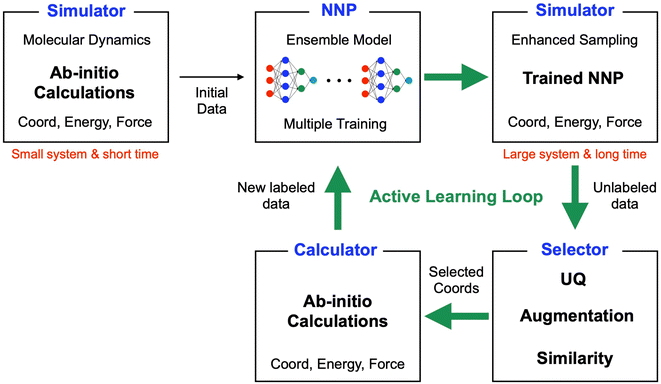
A schematic of the active learning process in the current study is shown in Fig. 1. The data selector in the AL loop is crucial in our study because it determines the quantity and quality of data, which directly impacts the NNP accuracy, the speed of the AL process, and the time required for calculations for new labeling. We employed a ‘query by committee’ algorithm for the UQ,³⁰ where the disagreement in an ensemble of NN models is used to estimate the reliability of the current data set. A previous study has shown that it effectively derives NNPs for organic molecules with conformal and configuration search¹⁵ although missing the capability of bond breaking. This study also estimates the UQ value through an ensemble of multiple models. Then, the selector utilizes the UQ value to choose new configurations for the following ab initio calculations. Unlike the previous study that used absolute values for the UQ criteria, we defined our criteria using the mean and standard deviation of UQ because the absolute values for the same configurations can change as more data are added.

Fig. 1 Schematic of the active learning process for neural network potentials proposed in the current study. Especially the workflow is designed for utilizing enhanced sampling methods through trained NNPs to capture rare events in atomistic simulations. The simulator is running MD with enhanced sampling, e.g., SMD using ab initio calculation or trained NNP. Multiple NNPs are trained for the ensemble approach. The selector selects configurational data for the following iteration. Utilizing only uncertainty quantification (UQ) values has limitations for screening valuable configurations for the following iteration. In addition to UQ estimation, we utilized data augmentation through random noise and similarity checks for efficient AL iterations.

The AL workflow involves numerous hyperparameters, such as the number of selected data included, the criteria of UQ, the number of ensemble models, etc. One major challenge to optimizing these parameters is the computational cost of labeling new data and retraining. Significantly, if all parameters are not optimized at the early stage of development, it becomes inevitable to perform lengthy ab initio calculations and retraining repeatedly. Therefore, selecting a test system and the methodology for labeling the new configurations identified through development becomes critical. We utilize a small finite-size molecular system, specifically hexane, one of the alkane chains. The alkane chains are simple, but testing such systems before investigating a more complex system is valuable and can provide useful insights for newly developed methods.³¹

Furthermore, the density functional-based tight binding (DFTB) approach,³² an approximate electronic structure method, overcomes the computational demands of density functional theory (DFT) in developing and demonstrating our AL process. We applied one enhanced sampling method, steered molecular dynamics (SMD),³³ to describe chemical bond breaking for the alkane chain under tensile loading. SMD utilizes an imaginary spring to apply an external force to an atom or a group of atoms, which allows us to study the dynamic behaviors of the system. The method has been widely utilized for protein systems^34,35 and nanomaterials^36–38 due to the natural behaviors of materials while applying external forces compared to directly moving atoms or groups.

During the AL process, we performed SMD simulations through trained NNPs. Not all configurations sampled through SMD with the initially trained NNP are valuable to be included in the subsequent iterations. One anticipated issue is that these configurations will have very similar structures because the sampling is based on the simulations with a short time step. Each sampled configuration is highly correlated with the previously sampled configurations. In the SMD simulations, the distance between one end to the other end of the molecule is a good indicator of structural similarity, as we utilized the spring distance as a collective variable representing the reaction path. One can choose other values for different applications, e.g., density, order parameters, and structural fingerprints, which should be well-designed for desired performance. Based on the spring distance, we can select a small number of configurations distinguished from each other well in each AL loop.

Another issue is that the sampled path via the inaccurate NNPs usually does not represent a correct path. To accurately learn the PES around the sampled configurations, additional data is required to guide whether the configurations are energetically favored. The additional configurations must be similar enough to the sampled ones. Otherwise, the NNPs cannot interpolate between the sampled and additional configurations. In this study, we augmented the configuration data by adding random noise to the coordinates of each atom in the sampled configurations.

2.2 Data generation

2.2.1 Steered molecular dynamics. We performed steered molecular dynamics (SMD)³⁹ for a hexane molecule (C₆H₁₄) via the LAMMPS package.⁴⁰ The interaction between atoms was described with the density functional tight binding (DFTB) method through the DFTB+ package,⁴¹ utilizing a previously developed interface for LAMMPS.⁴² We employed the 3OB⁴³ parameters with the DFTB3 scheme. The initial structure was relaxed at 10 K for 2000 steps through the Berendsen thermostat with a time step of 0.5 fs. After relaxation, an imaginary spring (spring constant, 10 eV Å⁻²) was attached to two carbon atoms at the edges, and then, the atoms were stretched with a velocity of 1 Å ps⁻¹ for 6500 steps. The low temperature was selected to estimate the activation energy for the chain breaking precisely by minimizing kinetic energy contribution. The recorded data, as unseen test data, is utilized to test the performance of trained NNPs during the active learning process. We performed the SMD simulation with trained NNPs under the same conditions, using a previously developed interface between PyTorch and LAMMPS.⁴⁴

2.2.2 Molecular dynamics. The initial model is trained from the sampled configurations through constant temperature simulation. We followed a conventional approach, running an MD simulation at a high temperature. We obtained 2000 data points at 500 K with a time step of 0.5 fs. This data set is for the first NNP model initiating the AL process. The previous section provides the correctly sampled configurations directly sampled from DFTB-based SMD simulation.

2.3 Active learning

Fig. 1 shows the schematic of the active learning process in this study. We prepared multiple ANI-based NNP models, performed an SMD simulation using the best model (the lowest MAE, Mean Absolute Error, of force components), and obtained the trajectories. From the configurations from SMD, we estimate each configuration's UQ values based on the energy predictions' standard deviation. At each active learning iteration, unique configurations are selected based on the similarity check and boosting configurations by adding random noise displacement. The energy of generated new configurations is calculated using a physics-based model and is incorporated into the training in the following active learning iteration. The performances of NNPs are also evaluated through the unseen DFTB-based SMD simulation data and the activation energy.

2.3.1 ANI neural network structure and training. We utilized the TorchANI²⁷ tool to train ANI-based NNPs from data sets. The detailed structures of the NN are listed in Table 1. In this model, atomic environmental vectors (AEV), or symmetry functions, G, are calculated from the coordinates (q) as input for the NN.²⁸ There are radial (atoms i and j with distance R_ij) and angular terms (atoms i, j, and k with two distances R_ij, R_ik, and one θ_ijk):²⁷where η governs the width of the Gaussian function with multiple R_s (m is an index for R_s); ζ governs the width of probing as η; θ_s decides the specific region in the angular environments as R_s. f_C is a cutoff function to change values to zero at R_C smoothly, defined as for R ≤ R_C and 0 for R > R_C.

Table 1 Neural network structures utilized for TorchANI in the current study. We followed the basic settings of ANI-2x (provided in TorchANI). Gaussian error linear unit activation function⁴⁸ was utilized to add non-linearity between AEV-1st, 1st–2nd, and 2nd–3rd layers

NN model	1st	2nd	3rd	Output (energy)
H	256	192	160	1
C	224	192	160	1

---

At each AL iteration, 80% of the data was used to train the model, and 20% was used for validation with a mini-batch size of 64. The data was shuffled when they were loaded. We followed the parameters of the AEV from ANI-2x⁴⁵ model.

The loss function is defined as

where α was set to 0.1, a parameter to determine the contribution of forces. The basic training conditions are the same as in the previous study.⁴⁴ We trained parameters with 300 epochs and took the best parameters for the MSE of energy with the validation set during the epochs. We did not prepare a test set during the active learning iterations. However, the performance of trained models was also measured through unseen data to check the generalization of the models at each AL iteration.

2.3.2 Uncertainty quantification. Uncertainty quantification (UQ) of the NNPs is a central part of active learning because it allows us to identify valuable data, which is likely to be informative and worth labeling with new calculations, distinguishing from the previous data set. In this study, we employ the ensemble-based approach, utilizing the same NNP structure but with different training and validation sets for each model. Then, energy is predicted from each model, and the standard deviation from the models' predictions is used as an uncertainty quantification (UQ) measure. The UQ values of the same sampling region can vary at each AL iteration (see Fig. S1‡). Therefore, instead of an absolute value for the UQ criteria, we utilized data from the initial 1000 steps of SMD simulation to calculate the mean (μ_UQ) and standard deviation (σ_UQ) of the UQ values. Then, we utilized the values of μ_UQ + 3σ_UQ as a criterion to decide whether the sampled configurations are new or not. For example, if the UQ value is larger than μ_UQ + 3σ_UQ, we consider the configuration is not included in the training and validation data set at the active learning iteration.

2.3.3 Similarity screening. Once an atomic bond breaks, the molecule is separated into two parts. From that stage, the local configurations of the broken parts maintain the similarity because no further stretching force is applied to the molecule. Those configurations may or may not be essential, so we set the maximum number (e.g., 50) of configurations to exclude too similar configurations, even with high UQ values. Also, during the stretching of the molecule before the bond breaking, the configuration of the molecule slowly changes. In contrast, the breaking process itself drastically changes the configurations in a short time. Therefore, including all the configurations based on the same time step would cause a data imbalance problem. To alleviate the problem, the spring distance was used to indicate the configurational similarity. We selected the data step by step to check the distance and energy differences between chosen configurations. All selected data for new labeling must satisfy the condition that the differences in energy and distance are larger than 1 kcal mol⁻¹ difference and 0.01 Å, respectively. A previous study applied a similar approach to graphene fracture to address the data imbalance problem.⁴⁴

2.3.4 Configuration augmentation. To improve the generalization of NNPs, learning the potential energy surface is critical rather than memorizing energy values at specific configurations. SMD simulation guides the molecule to deform through a very narrow path, and in the early stages of the AL iterations, the guided path is not energetically favorable. Therefore, verifying if the predicted path is appropriate is essential by labeling configurations near the path. Empirically, NNPs perform better with data augmentation, especially after bond breaking (see ESI Note 1‡). Therefore, we added random (uniform) noise (max/min ±0.05 Å) to the coordinates of atoms along each axis for NNP to learn the potential energy surface near the sampled point (e.g., two more configurations).

2.3.5 SchNet training. SchNet is a neural network based on continuous-filter convolutions. It first builds embedding vectors from the atom type and includes the configurations through a series of interaction blocks. SchNet performs incredibly for the energy/force predictions from the atomic structures and other properties of molecules/crystals, e.g., HOMO LUMO or band gaps, dipole moment, zero-point vibrational energy, etc.⁴⁶ In the current study, we utilized SchNet only for the energy/force prediction of the molecule. The detailed structures are listed in Table 2. The loss function is composed of energy and force loss based on the mean square errors as

Loss = ρ × MSE (energy) + (1 − ρ) × MSE (force) (4)

where we set ρ as 0.1. The total number of epochs was 300. We trained the models based on the functions provided in the SchNet package.²⁹ The Adam optimizer was utilized with a learning rate (lr) scheduler (a function “reduced lr on plateau”) with factor = 0.8, patience = 5, min_lr = 1 × 10⁻⁶, initially lr = 5 × 10⁻⁴. We took the best model for the validation set during the entire epochs, and training is stopped if lr reaches the minimum lr. The achieved accuracy of the training/validation sets of the equilibrium data set 2000 is 0.29 kcal mol⁻¹ (±0.037 kcal mol⁻¹). The MAE of energy depends on the ρ value. We can set ρ as 0.01, as the previous study suggested, but the unphysical behaviors under tensile loading were unresolved. We note that the loss functions of TorchANI and SchNet have different forms based on their original development. We followed the setting suggested for weights between energy and force, e.g., more weight for energy in TorchANI training and more weight for force in SchNet training. Our current conditions work well for training 2000 data points and the configuration data sampled from the active learning with TorchANI.

Table 2 The setup of SchNet utilized in the current study

	# Features	# Gaussian	# Interaction	Cutoff (Å)
Values	128	25	3	5

---

2.3.6 Inherited data selection. The ensemble models are trained through randomly selected training/validation sets from the same data. Although the MAE of training/validation has a small variance (e.g., the variance of three ensembles at AL 9 is less than 0.005 eV), the activation energy obtained from SMD simulations can vary much more than that (∼0.25 eV > 24 kcal mol⁻¹). An apparent training uncertainty exists; therefore, we designed a different strategy from the random selection to stabilize the performance of models. The inherited selection strategy takes the training/validation sets from the previously selected sets, showing the best performance based on the error of forces prediction of the entire data set (training + validation sets). Only newly imported data sets are randomly distributed in each ensemble training. This strategy better stabilizes the convergence of the activation energy from SMD as the number of ensembles increases.

3. Results and discussions

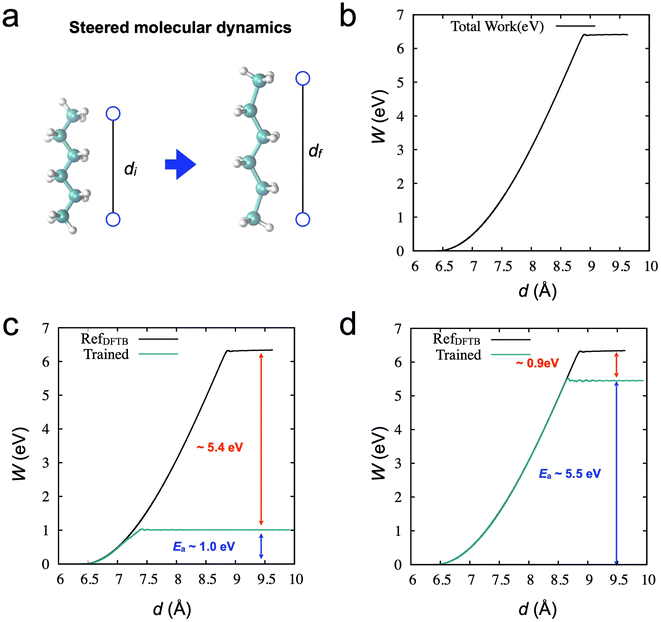
First, we performed an SMD simulation of the hexane molecule using DFTB calculation, as shown in Fig. 2. In the simulation, an imaginary spring is attached to two carbon atoms at the edges, as shown in Fig. 2a. During the SMD simulation, the spring distance increases from around 6.5 Å to 9.5 Å (6500 steps). The work (W) done by the spring, as a function of the spring distance, is obtained in Fig. 2b. The activation energy for the chain breaking is about 6.34 eV.

Fig. 2 (a) Steered molecular dynamics simulation of stretching a hexane molecule. (b) Obtained work function through the spring elongation as a function of spring distance. The maximum energy for bond breaking requires around 6.4 eV. (c) Result of SMD through the trained model based on the 2000 MD data. Since the NVT ensemble does not include elongated configurations, the error of the energy barrier is huge, 5.4 eV. (d) Results of SMD through the trained model based on the 6500 DFTB-based SMD data. Although the data set includes the entire trajectories, there is still a non-negligible amount of error, 0.9 eV.

To train the initial NNP models for active learning, we prepared a data set from the equilibrium state from a conventional MD simulation at 500 K (2000 steps, see Method). Fig. 2c shows the results of SMD simulation through the trained NNPs from the data set. As expected, the NNP from the equilibrium data cannot adequately describe the molecule's deformation (or stretching), and failure occurs at a short spring distance of around 7.5 Å. Although the NNP accurately describes the potential curve near the equilibrium position, the obtained activation energy is only 1.0 eV. On the other hand, we also trained the NNP from the SMD data points (6500). This data set could more accurately describe the deformation with a better estimation of the activation energy ∼5.5 eV in Fig. 2d. However, the error of the activation energy is still significant, ∼0.9 eV (∼20 kcal mol⁻¹). These observations are consistent with a previous study on graphene fracture.⁴⁴ The trained model from the equilibrium states could not describe the graphene's fracture. Also, the data obtained from a single fracture simulation is insufficient to train the NNP to accurately describe the properties of graphene fracture, e.g., strength and bond-breaking processes.

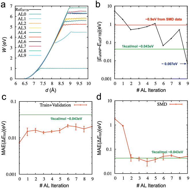
The aim of our active learning process is to obtain valuable newly labeled data by enhanced sampling through trained NNP models, not by directly sampled data from DFT or DFTB calculations. We initially performed ten iterations of the designed active learning (see Method) from the 2000 initial data points. In the process we designed, the SMD simulations were performed using trained NNPs, rather than the DFT/DFTB. Fig. 3a shows the work functions from the SMD simulations as a function of spring distance from the initial NNP to the final NNP. The work functions get close to the correct answer (black line), and the error of the activation energy for chain breaking becomes lower than 1 kcal mol⁻¹ in Fig. 3b. For each active learning iteration, we added 150 new data. Therefore, the final NNP was trained using only 3350 data points. Given that the error is about 0.9 eV (∼20 kcal mol⁻¹) from the NNP trained by the SMD data (6500), the performance (the error is about 0.007 eV, ∼0.16 kcal mol⁻¹) of the final NNP is excellent. It should be noted that the error does not monotonically decrease but shows a fluctuation. One of the reasons for the oscillation is the presence of inaccurate sampling paths. There are states where the error increases or does not decrease significantly. In those states, the early-stage NNP searches for wrong reaction paths until the newly labeled data indicate that the paths are not energetically favorable. Another reason comes from training uncertainty, which will be discussed later.

Fig. 3 Active learning (AL) results based on TorchANI models: (a) the work function of the best model from three models with the random selection strategy. (b) Absolute error (|E_aNNP − E_aDFTB|) of the best model trained and selected at each AL iteration (c) MAE of the relative energy during the active learning based on the train/validation data at each iteration (d) MAE of the relative energy during the active learning based on the unseen SMD data (6500 points).

Fig. 3c shows the MAE values of the relative energy from the training and validation data sets at each iteration. The error increases from the initial model trained with 2000 data points as the new data are included in the data set. This further confirms that the accuracy of training and validation does not guarantee any physically reasonable behaviors of the systems. As we evaluate the models based on the unseen data set from the DFTB-based SMD simulation (6500 data points), the accuracy significantly improves once the data acquired from the active learning was added until 2nd iteration. However, the accuracy does not improve but fluctuates around 1 kcal mol⁻¹ after the 3rd iteration. There is little correlation between the activation energy and SMD data accuracy. This also suggests that the SMD data from the DFTB-based simulation does not provide enough configurations for training NNP to describe the failure process appropriately and why it is essential to check the physical properties of the trained models.

The current active learning process can offer significant advantages over the enhanced sampling through ab initio calculations as the system becomes complicated. SMD simulations require sequential time integration for the dynamic process. This cannot be easily parallelized as the following configuration depends on a previous configuration. For example, if each configuration calculation through DFT takes one minute, the entire SMD simulation (6500 sequential integrations) takes about 4.5 days. However, the obtained configurations from active learning can be newly labeled through the DFT calculation with embarrassing parallelization. Therefore, the most time-consuming part of active learning is training the models. For example, 2000–4000 data training takes about an hour using one GPU. Based on the above assumptions, the time for obtaining an accurate reaction barrier through SMD can be reduced to 10% of DFT-based calculations. The advantage becomes more critical as the system complexity increases, making it practical for more complex and larger atomistic simulations with DFT accuracy.

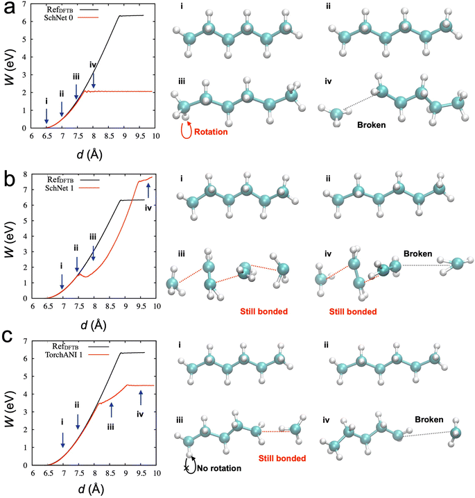
We investigated whether the same developed process can be transferable to other types of NNP. We hypothesized that critical configurations for training to describe appropriate physical behaviors should be similar, and the configurations can be distinguished in the developed active learning process. To test our hypothesis, we utilized SchNet,²⁹ another type of NNP, showing high performance in terms of accuracy of energy and forces, but we could not obtain the desirable behaviors from SchNet. Table 2 lists the parameters for the SchNet structure and training in the current study. Fig. 4a shows the SMD results from the initial model trained from the 2000 data points. The configuration snapshots show reasonable behaviors of stretching and breaking one of the C–C bonds, which is consistent with SMD simulation through DFTB. The activation energy for the bond breaking is about 2 eV, which is better than TorchANI model (∼1 eV). However, after the acquisition of the 1st data (150 points), the SchNet model showed unphysical configurations in Fig. 4b. Snapshot (iii) in Fig. 4b shows two different bond lengths between two carbon atoms. After one of the C–C bonds breaks at the spring distance of about 9.5 Å, the configuration does not recover to the configuration as in Fig. 4a (iv). On the other hand, the TorchANI model shows better behaviors in Fig. 4c after the 1st active learning iteration. Although it results in an unphysical bond length in the snapshot (iii) in Fig. 4c, it does not show the local minimum as SchNet. In later iterations of TorchANI-based active learning, this long bond length is adjusted by labeling the new data. We could not successfully apply iterative active learning with SchNet because the trained models became unstable during SMD simulations, breaking down into several pieces. We further investigated where the difference between SchNet and TorchANI arises. We realized that the challenge did not originate from training conditions (e.g., cutoff) for SchNet but happened when SchNet tried to learn the sampled configuration by the SchNet (see ESI Note 2‡). Our observations also remind us that just errors of energy and force cannot evaluate the reliability of ML-based interatomic potential models.⁴⁷

Fig. 4 (a) Results of SMD simulation from the initial SchNet model without active learning. (b) Results of SMD simulation from the SchNet model trained from 1st active learning iteration. (c) Results of SMD simulation from the ANI model trained from 1st active learning (see Movies 1 and 2 for panels b and c).

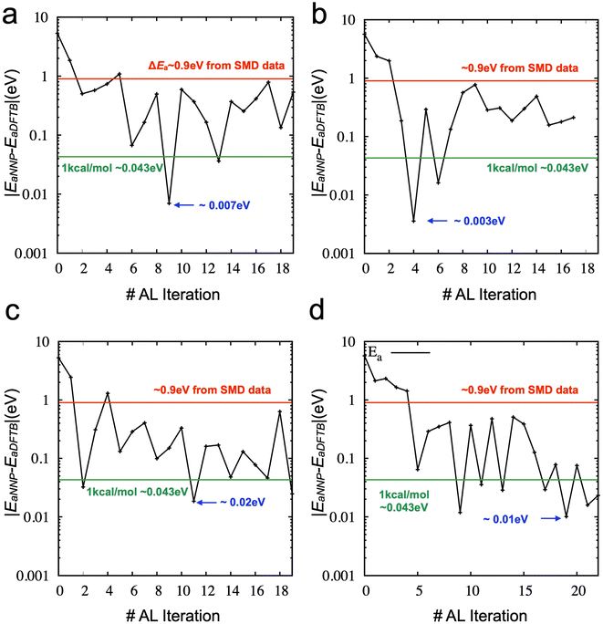
Then, we explored the stability of training by performing further iterations of active learning. Fig. S2‡ shows the results of active learning iterations from the 9th to the 19th. We observed that the accuracy of the activation energy was unstable. Such instability is not ideal for the practical applications of active learning because the convergence of physical quantity (here, the activation energy for chain breaking) is the only reliable indicator. We found that SMD simulations and the derived activation energy can change due to the different training/validation sets from additional tests. In other words, the NNP's performance could fluctuate if we mixed the data into different training/validation sets. Therefore, we proposed a new strategy (see Method) as the training/validation sets showing the most promising performance are carried forward to the following iteration. The direct comparison between the two strategies (one is the random selection of training/validation sets at each iteration, and the other is the inherited selection of training/validation sets from the previous iteration) is shown in Fig. 5a and b (see also Fig. S3‡). It demonstrates that using the inherited data selection reduces fluctuations in the error. However, the converged error is now significant (∼0.2 eV), although it still presents an improvement over the model trained from DFTB-based SMD data sets (∼0.9 eV). We increase the number of ensembles from three to five and seven and draw the error of activation energies, as shown in Fig. 5c and d (see also Fig. S4 and S5‡). We added three more iterations for the seven ensembles to confirm the convergence. The results suggest that more models of the ensemble can enhance the convergence of the activation energy with a very high accuracy.

Fig. 5 Absolute error (|E_aNNP − E_aDFTB|) of the best model trained and selected at each AL iteration based on the TorchANI models: (a) an ensemble includes three models with the random selection strategy. (b) Three models with the inherited selection strategy (c) five models with the inherited selection strategy. (d) Seven models with the inherited selection strategy.

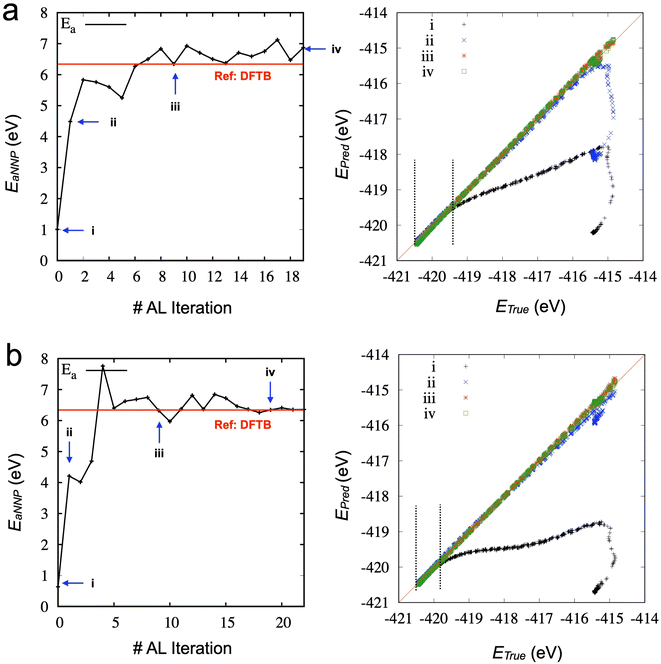
Fig. 6 compares the activation energy and accuracy for the SMD data (unseen data) from DFTB between random selections (# of ensembles = 3) and transferred selections (# of ensembles = 7). Interestingly, the initial trained model (curve (i), 0th iteration) of the random selection predicts the unseen data better than the inherited selection. Since we selected the best models based on the error of force components to avoid overfitting, more ensembles provide a better model but do not necessarily perform better in energy prediction. However, in the 1st iteration, the inherited selection with a larger number of ensembles covers more relevant data (blue curves, (ii)). We can interpret that a less overfitted model can find a path through the SMD in the next iteration, helping to find the correct reaction path and faster convergence of the activation energy estimation (see also Fig. S6‡).

Fig. 6 (left) Activation energy obtained from trained TorchANI-based SMD simulations during the active learning. (right) Scattering plots of unseen data points (6500 points) from DFTB-based SMD simulation. The results from different strategies for training/validation data sets: (a) the random selection strategy from the entire data at each iteration with three models. (b) The inherited selection strategy with seven models. Only newly imported configurations at each AL iteration are randomly distributed. The dotted lines indicate the ranges of aligned energy values with the predictions from the initial TorchANI model (without AL).

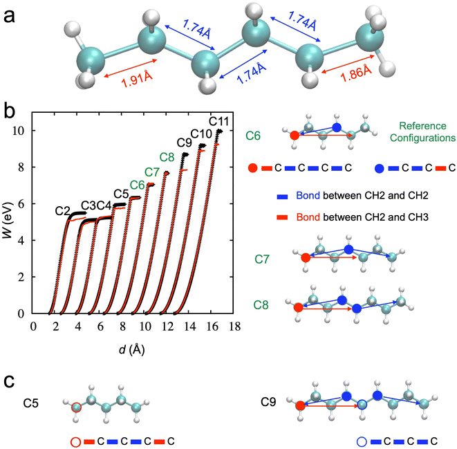
Finally, we tested the transferability of the trained NNP. Fig. 7a shows the lengths of the CH₃–CH₂ bonds at the terminals (or the edges) are different from those of CH₂–CH₂ bonds near the breaking point from DFTB. Since the stretching of the hexane chain includes 5 C–C bonds simultaneously, it is hard to expect the bond-breaking of individual C–C to be learned well. For example, stretching one in the middle or one in the edge but fully relaxing other bonds is not included in the data set.

Fig. 7 (a) Bond lengths of each C–C bond in the hexane chain near the breaking points. There are two types of bonds: one is CH₃–CH₂ (red line in panel b), and the other one is CH₂–CH₂ (blue line in panel b). (b) SMD simulations from C₂ to C₁₁ by the NNP (TorchANI model) trained from the AL for the hexane chains. The black dotted lines are obtained from DFTB, and the red lines are obtained through the trained NNP (TorchANI model) with a hexane chain. Only C₇ and C₈ show good estimations of the activation energy. Two different bond groups, starting from red closed-circled carbon and blue closed-circled carbon, are the longest bond groups under deformation. These two groups can still describe the longest bond groups under the deformation of the C₇ and C₈ chains. (c) However, new bond group emergs as the chain becomes shorter (e.g., C₅ in pane c) or longer than C₈ (e.g., C₉ in panel c). This can provide insight into how the transferability of NNP (TorchANI model) works.

We should consider the stretching of the hexane chain based on the deformation in the group of bonds in addition to the individual bonds to understand how NNP works. To demonstrate this more clearly, we performed additional simulations with other chains from ethane (C₂) to undecane (C₁₁) to check the transferability of NNP derived from the hexane to other chains. Fig. 7b shows the results; only C₇ and C₈ can be well described compared to other chains.

We note that there are two distinct bond groups within the radius cutoff for the BP symmetry function in the hexane chain: one starts from the carbon at the edge (CH₃, red closed-circle), and the other starts from the carbon in the middle (CH₂, blue closed-circle). The deformation of chains C₇ and C₈, the longest bond groups, can still be covered by these two bond groups in the hexane chain.

However, a new bond group, starting from the red open-circled carbon, emerges when the chain gets short (e.g., C₅), as shown in Fig. 7c. Also, a new bond group, starting from the blue open-circled carbon, shows up as the chain gets longer (e.g., C₉). Therefore, the accuracy of the activation energy decreases, and the transferability is only validated in limited cases.

We further check the strain rate effects. Once the simulation conditions change, the accuracy is not guaranteed and rechecked because the new conditions may sample new configurations for the bond breaking. We performed additional simulations and compared them with DFTB simulations for the different loading rates to see how much the performance can change, as in Fig. S7.‡ As we expected, the breaking point and activation energy slightly deviate from the reference calculations. Still, they could capture the trend of strain rate effects, e.g., higher energy and longer breaking distance for a higher strain rate.

The approach we developed in the study offers a practical way to accurately estimate the activation energy, although further investigations are required for broader applications.

4. Conclusion

In summary, we proposed and developed an active learning workflow with enhanced sampling techniques in molecular dynamics for neural network potentials. Although the initial training set is obtained from the conventional MD sampling at the equilibrium state, our developed active learning process rapidly collects data that covers the essential configuration of hexane chain breaking under the loading condition, thus achieving high accuracy in the estimation of the activation energy, with an error of approximately 1 kcal mol⁻¹. However, the activation energy from the trained NNPs through SMD was not likely to converge. We devised and applied the inherited data selection strategy to improve convergence. Although there is room for further optimizations, e.g., the number of new data, a way of boosting configurations, similarity checks, and utilizing UQ values, our approach provides a successful reference for future research. Our study will benefit more realistic and complex systems and further development of NNP for various applications related to catalysis, chemical reactions, and phase transitions.

Data availability

All data needed to evaluate the conclusions in the paper are present in the paper and/or the ESI.‡ Extra data and machine-readable data are available upon reasonable request to the authors.

Code availability

Sample inputs and source codes of the active learning in the current case study are available at https://github.com/ORNL/al-asmr. The code for TorchANI can be found at https://github.com/aiqm/torchani. The code for SchNet can be found at https://github.com/atomistic-machine-learning/schnetpack. The code for the interface between LAMMPS and DFTB+ can be found at https://github.com/gsjung0419/DFTBP; DOI: https://doi.org/10.1016/j.carbon.2022.01.002. The code for the interface between LAMMPS and TorchANI can be found at https://github.com/gsjung0419/LMPTorch and https://github.com/gsjung0419/LammpsANI; DOI: https://doi.org/10.1088/2632-2153/accd45.

Author contributions

G. S. J. conceived the idea, developed codes, generated data, performed experiments, and analyzed results. G. S. J, J. Y. C, and S. K. L. tested, optimized the codes, and wrote and edited the manuscript.

Conflicts of interest

The authors have no conflicts of interest to declare.

Acknowledgements

The authors acknowledge support by the Artificial Intelligence Initiative exploratory project as part of the Laboratory Directed Research and Development Program (LDRD) of Oak Ridge National Laboratory, managed by UT-Battelle, LLC, for the US Department of Energy under contract DE-AC05-00OR22725. This research used resources of the Compute and Data Environment for Science (CADES) at the Oak Ridge National Laboratory, which is supported by the Office of Science of the U.S. Department of Energy under Contract No. DE-AC05-00OR22725.

References

1. J. Jumper, R. Evans, A. Pritzel, T. Green, M. Figurnov and O. Ronneberger, et al., Highly accurate protein structure prediction with AlphaFold, Nature, 2021, 596(7873), 583–589.
2. J. Schmidt, M. R. G. Marques, S. Botti and M. A. L. Marques, Recent advances and applications of machine learning in solid-state materials science, npj Comput. Mater., 2019, 5(1), 83.
3. K. T. Butler, D. W. Davies, H. Cartwright, O. Isayev and A. Walsh, Machine learning for molecular and materials science, Nature, 2018, 559(7715), 547–555.
4. D. Pfau, J. S. Spencer, A. G. D. G. Matthews and W. M. C. Foulkes, Ab initio solution of the many-electron Schrödinger equation with deep neural networks, Phys. Rev. Res., 2020, 2(3), 033429.
5. J. Vamathevan, D. Clark, P. Czodrowski, I. Dunham, E. Ferran and G. Lee, et al., Applications of machine learning in drug discovery and development, Nat. Rev. Drug Discovery, 2019, 18(6), 463–477.
6. H. Wang, T. Fu, Y. Du, W. Gao, K. Huang and Z. Liu, et al., Scientific discovery in the age of artificial intelligence, Nature, 2023, 620(7972), 47–60.
7. K. Alberi, M. B. Nardelli, A. Zakutayev, L. Mitas, S. Curtarolo and A. Jain, et al., The 2019 materials by design roadmap, J. Phys. D: Appl. Phys., 2018, 52(1), 013001.
8. A. Chen, X. Zhang and Z. Zhou, Machine learning: Accelerating materials development for energy storage and conversion, InfoMat, 2020, 2(3), 553–576.
9. J. Behler and G. Csányi, Machine learning potentials for extended systems: a perspective, Eur. Phys. J. B, 2021, 94(7), 142.
10. E. Kocer, T. W. Ko and J. Behler, Neural Network Potentials: A Concise Overview of Methods, Annu. Rev. Phys. Chem., 2022, 73, 163–186.
11. M. Pinheiro, F. Ge, N. Ferré, P. O. Dral and M. Barbatti, Choosing the right molecular machine learning potential, Chem. Sci., 2021, 12(43), 14396–14413.
12. O. T. Unke, S. Chmiela, H. E. Sauceda, M. Gastegger, I. Poltavsky and K. T. Schütt, et al., Machine Learning Force Fields, Chem. Rev., 2021, 121(16), 10142–10186.
13. S. Lorenz, A. Groß and M. Scheffler, Representing high-dimensional potential-energy surfaces for reactions at surfaces by neural networks, Chem. Phys. Lett., 2004, 395(4–6), 210–215.
14. B. Settles, Active Learning Literature Survey, 2009.
15. J. S. Smith, B. Nebgen, N. Lubbers, O. Isayev and A. E. Roitberg, Less is more: Sampling chemical space with active learning, J. Chem. Phys., 2018, 148(24), 241733.
16. J. S. Smith, B. Nebgen, N. Mathew, J. Chen, N. Lubbers and L. Burakovsky, et al., Automated discovery of a robust interatomic potential for aluminum, Nat. Commun., 2021, 12(1), 1257.
17. V. Botu and R. Ramprasad, Adaptive machine learning framework to accelerate ab initio molecular dynamics, Int. J. Quantum Chem., 2015, 115(16), 1074–1083.
18. S. J. Ang, W. Wang, D. Schwalbe-Koda, S. Axelrod and R. Gómez-Bombarelli, Active learning accelerates ab initio molecular dynamics on reactive energy surfaces, Chem, 2021, 7(3), 738–751.
19. A. A. Peterson, R. Christensen and A. Khorshidi, Addressing uncertainty in atomistic machine learning, Phys. Chem. Chem. Phys., 2017, 19(18), 10978–10985.
20. B. Charles, C. Julien, K. Koray and W. Daan, Weight Uncertainty in Neural Network, PMLR, 2015, pp. 1613–1622.
21. G. Yarin and G. Zoubin, Dropout as a Bayesian Approximation: Representing Model Uncertainty in Deep Learning, PMLR, 2016, pp. 1050–1059.
22. A survey of neural network ensembles, International Conference on Neural Networks and Brain, ed. Z. Ying, G. Jun and Y. Xuezhi, 2005.
23. D. Schwalbe-Koda, A. R. Tan and R. Gómez-Bombarelli, Differentiable sampling of molecular geometries with uncertainty-based adversarial attacks, Nat. Commun., 2021, 12(1), 5104.
24. S. Izrailev, S. Stepaniants, M. Balsera, Y. Oono and K. Schulten, Molecular dynamics study of unbinding of the avidin-biotin complex, Biophys. J., 1997, 72(4), 1568–1581.
25. R. C. Bernardi, M. C. R. Melo and K. Schulten, Enhanced sampling techniques in molecular dynamics simulations of biological systems, Biochim. Biophys. Acta, Gen. Subj., 2015, 1850(5), 872–877.
26. Y. I. Yang, Q. Shao, J. Zhang, L. Yang and Y. Q. Gao, Enhanced sampling in molecular dynamics, J. Chem. Phys., 2019, 151(7), 070902.
27. X. Gao, F. Ramezanghorbani, O. Isayev, J. S. Smith and A. E. Roitberg, TorchANI: A Free and Open Source PyTorch-Based Deep Learning Implementation of the ANI Neural Network Potentials, J. Chem. Inf. Model., 2020, 60(7), 3408–3415.
28. J. Behler and M. Parrinello, Generalized Neural-Network Representation of High-Dimensional Potential-Energy Surfaces, Phys. Rev. Lett., 2007, 98(14), 146401.
29. K. T. Schütt, P. Kessel, M. Gastegger, K. A. Nicoli, A. Tkatchenko and K. R. Müller, SchNetPack: A Deep Learning Toolbox For Atomistic Systems, J. Chem. Theory Comput., 2019, 15(1), 448–455.
30. H. S. Seung, M. Opper, H. Sompolinsky and Query by committee, Proceedings of the fifth annual workshop on Computational learning theory, Association for Computing Machinery, Pittsburgh, Pennsylvania, USA, 1992, pp. 287–94.
31. Q. H. Hu, A. M. Johannesen, D. S. Graham and J. D. Goodpaster, Neural network potentials for reactive chemistry: CASPT2 quality potential energy surfaces for bond breaking, Digital Discovery, 2023, 2(4), 1058–1069.
32. M. Gaus, Q. Cui and M. Elstner, DFTB3: Extension of the Self-Consistent-Charge Density-Functional Tight-Binding Method (SCC-DFTB), J. Chem. Theory Comput., 2011, 7(4), 931–948.
33. L. Y. Chen, Exploring the free-energy landscapes of biological systems with steered molecular dynamics, Phys. Chem. Chem. Phys., 2011, 13(13), 6176–6183.
34. J. L. Zitnay, G. S. Jung, A. H. Lin, Z. Qin, Y. Li and S. M. Yu, et al., Accumulation of collagen molecular unfolding is the mechanism of cyclic fatigue damage and failure in collagenous tissues, Sci. Adv., 2020, 6(35), eaba2795.
35. J. Yeo, G. Jung, A. Tarakanova, F. J. Martín-Martínez, Z. Qin and Y. Cheng, et al., Multiscale modeling of keratin, collagen, elastin and related human diseases: Perspectives from atomistic to coarse-grained molecular dynamics simulations, Extreme Mech. Lett., 2018, 20, 112–124.
36. E. Beniash, C. A. Stifler, C.-Y. Sun, G. S. Jung, Z. Qin and M. J. Buehler, et al., The hidden structure of human enamel, Nat. Commun., 2019, 10(1), 4383.
37. G. S. Jung, S. Wang, Z. Qin, F. J. Martin-Martinez, J. H. Warner and M. J. Buehler, Interlocking Friction Governs the Mechanical Fracture of Bilayer MoS2, ACS Nano, 2018, 12(4), 3600–3608.
38. G. H. Ryu, G. S. Jung, H. Park, R.-J. Chang and J. H. Warner, Atomistic Mechanics of Torn Back Folded Edges of Triangular Voids in Monolayer WS2, Small, 2021, 2104238.
39. Steered molecular dynamics, Computational Molecular Dynamics: Challenges, Methods, Ideas: Proceedings of the 2nd International Symposium on Algorithms for Macromolecular Modelling, ed. S. Izrailev, S. Stepaniants, B. Isralewitz, D. Kosztin, H. Lu, F. Molnar, et al., Springer, Berlin, 1999.
40. S. Plimpton, Fast Parallel Algorithms for Short-Range Molecular Dynamics, J. Comput. Phys., 1995, 117(1), 1–19.
41. B. Hourahine, B. Aradi, V. Blum, F. Bonafé, A. Buccheri and C. Camacho, et al., DFTB+, a software package for efficient approximate density functional theory based atomistic simulations, J. Chem. Phys., 2020, 152(12), 124101.
42. G. S. Jung, S. Irle and B. G. Sumpter, Dynamic aspects of graphene deformation and fracture from approximate density functional theory, Carbon, 2022, 190, 183–193.
43. M. Gaus, A. Goez and M. Elstner, Parametrization and Benchmark of DFTB3 for Organic Molecules, J. Chem. Theory Comput., 2013, 9(1), 338–354.
44. G. S. Jung, H. Myung and S. Irle, Artificial neural network potentials for mechanics and fracture dynamics of two-dimensional crystals, Mach. learn.: sci. technol., 2023, 4(3), 035001.
45. C. Devereux, J. S. Smith, K. K. Huddleston, K. Barros, R. Zubatyuk and O. Isayev, et al., Extending the Applicability of the ANI Deep Learning Molecular Potential to Sulfur and Halogens, J. Chem. Theory Comput., 2020, 16(7), 4192–4202.
46. P. B. Jørgensen, K. W. Jacobsen and M. N. Schmidt, Neural message passing with edge updates for predicting properties of molecules and materials, arXiv, 2018, preprint, arXiv:180603146,  DOI:10.48550/arXiv.1806.03146.
47. X. Fu, Z. Wu, W. Wang, T. Xie, S. Keten, R. Gomez-Bombarelli, et al., Forces are not Enough: Benchmark and Critical Evaluation for Machine Learning Force Fields with Molecular Simulations, 2022, arXiv, preprint, arXiv:221007237,  DOI:10.48550/arXiv.2210.07237.
48. D. Hendrycks and K. Gimpel, Gaussian Error Linear Units (GELUs), arXiv [csLG], 2020, preprint,  DOI:10.48550/arXiv.1606.08415.

---

Footnotes

† This manuscript has been authored by UT-Battelle, LLC, under contract DE-AC05-00OR22725 with the US Department of Energy (DOE). The US government retains and the publisher, by accepting the article for publication, acknowledges that the US government retains a nonexclusive, paid-up, irrevocable, worldwide license to publish or reproduce the published form of this manuscript, or allow others to do so, for US government purposes. DOE will provide public access to these results of federally sponsored research in accordance with the DOE Public Access Plan (http://energy.gov/downloads/doe-public-access-plan).

‡ Electronic supplementary information (ESI) available: Fig. S1–S10, supplementary notes 1 and 2. See DOI: https://doi.org/10.1039/d3dd00216k

---