Extrapolation validation (EV): a universal validation method for mitigating machine learning extrapolation risk

Abstract

Machine learning (ML) can provide decision-making advice for major challenges in science and engineering, and its rapid development has led to advances in fields like chemistry & medicine, earth & life sciences, and communications & transportation. Grasping the trustworthiness of the decision-making advice given by ML models remains challenging, especially when applying them to samples outside the domain-of-application. Here, an untrustworthy application situation (i.e., complete extrapolation-failure) that would occur in models developed by ML methods involving tree algorithms is confirmed, and the root cause of its difficulty in discovering novel materials & chemicals is revealed. Furthermore, a universal extrapolation risk evaluation scheme, termed the extrapolation validation (EV) method, is proposed, which is not restricted to specific ML methods and model architecture in its applicability. The EV method quantitatively evaluates the extrapolation ability of 11 popularly applied ML methods and digitalizes the extrapolation risk arising from variations of the independent variables in each method. Meanwhile, the EV method provides insights and solutions for evaluating the reliability of out-of-distribution sample prediction and selecting trustworthy ML methods.

---

1 Introduction

Machine learning (ML) has made impressive achievements in substance discovery, data analysis, and image processing over the past decades, accelerating advances in fields as numerous as earth & life science,^1–3 communications & transportation,^4–10 and chemistry & medicine.^11–20 As a spotlight to the field of chemistry, ML provides experimentalists with advice on selecting target molecules for synthesis by predicting physicochemical properties,^11–15 biological effects,^16–18 and reaction routes.^21–24 Although ML models are still not a complete substitute for expert intuition,²⁵ they are sufficiently sophisticated to recognize complex patterns beyond the reach of expert intuition to provide decision-making advice for major challenges in science and engineering, as multiple algorithms and different architectures for ML solutions emerge.^26–29

Grasping the trustworthiness of the decision-making advice given by ML models remains challenging.^30–33 Influencing the trustworthiness of model decision-making involves the whole process of modeling, i.e., not only the preparation of data but also the process of algorithm selection, hyper-parameterization, etc.³⁴ The accurate prediction of previously unknown things and the generation of reasonable decisions by ML models are derived from the data information available during development. As such, model uncertainty arising from the range of data and its distribution may lead to models making unconvincing (high-risk) decisions. For example, Li et al.³⁵ discovered that ML models trained on Materials Project 2018 may have severely degraded performance when predicting new compounds for Materials Project 2021, which was attributed to the changes in the distribution of the dataset.

Undoubtedly, if the prediction samples are located inside or on the boundary of the convex hull of the training dataset, the model prediction ability approximates its interpolation ability; if the prediction samples are located outside the convex hull, the model prediction ability depends on its extrapolation ability.³⁶ Thus, on any high-dimensional dataset, interpolation will almost certainly not occur, and model predictability will be more dependent on the extrapolation ability.^36,37 For the field of chemistry, the feature space is usually defined by the range of descriptors or the distribution of groups for the molecule.³⁸ The number of descriptors or groups corresponds to the dimension of the feature space. Indeed, an intersection of the prediction samples with the training dataset in one or more dimensions is possible,³⁹ and it is hard to assess the extent of the intersection, which is a source of model uncertainty.

Model uncertainty can be estimated using cross-validation and external validation tools.^{33,34,40–42} External validation is performed on data not involved in modeling. Cross-validation divides the training set according to various data partitioning schemes (e.g., random, leave-one-out, cluster, or time-split⁴³) to evaluate the performance of the model in future applications. For example, Meredig et al.⁴⁴ proposed the leave-one cluster-out cross-validation method (LOCO CV), which is based on the K-means clustering algorithm and classifies the samples into multiple clusters, and then divides the training and test sets according to the clusters. The k-fold-m-step forward cross-validation (kmFCV) proposed by Xiong et al.⁴⁵ divides the training and test sets according to the sequence of target values. Worth considering, the property distribution of molecules in the training set may not be identical to the distribution of molecules encountered in the future, i.e., molecules encountered in the future may be outside of the domain-of-applicability of the model. In time-split cross-validation, the model is trained on data generated before a certain date and tested on a retained dataset generated after that date. Thus, the time-split cross-validation method is deemed to be closer to the evaluation of new discoveries, i.e., prospective validation.^34,46 Due to data availability constraints, it may be difficult to obtain data that conform to this approach in certain cases.

While cross-validation and external validation provide an important tool for testing the potential utility of ML workflows, they are unable to distinguish between the predictions for in-domain and out-of-domain samples, which makes it hard to provide a quantitative evaluation of the extrapolation ability of an ML model. The consequences would be inconceivable if ML model extrapolation performance degradation, even extrapolation failure, occurs in artificial intelligence (AI)-driven applications, especially in high-risk scenarios such as self-driving cars, automated financial transactions, and smart healthcare. Hence, a method for quantitatively evaluating the extrapolation ability of a model is desired to reasonably circumvent the extrapolation risk.

Here, 11 ML methods are tested for out-of-domain sample prediction results on datasets with linear univariate, linear multivariate, and nonlinear multivariate functional relationships. Based on the extrapolation results, the involvement of the tree algorithm is suspected as the prime culprit in the extrapolation-failure of the ML model. Subsequently, the potential reasons are explored by using the random forest (RF) method as an example. To quantitatively evaluate the extrapolation ability, an extrapolation validation (EV) method is proposed. The EV method is applied to ML models with data from deterministic functional relationships, and the quantitative structural property relationship models for glass transition temperature (T_g) of polyimide (PI) in the macromolecular field as a real-world application example.

2 Methodology

2.1 Mathematical model extrapolation test

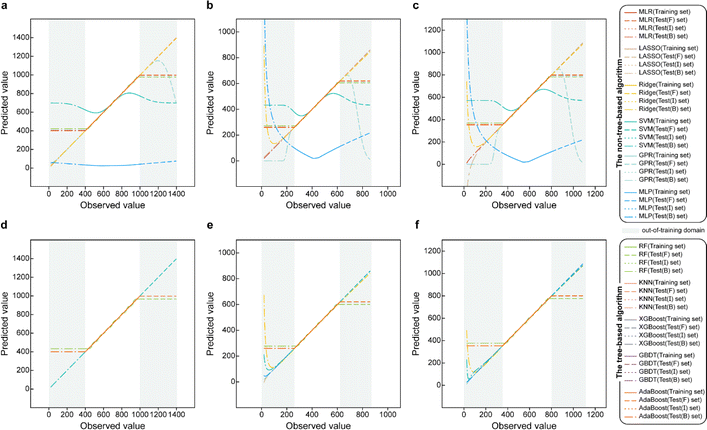
To obtain modeling data with clear functional relationships, five variables related to the x are defined, see eqn (1)–(5). With the tolerance of 2, the arithmetic sequence in the range of (400, 1000), (488, 888), (20, 400), and (1000, 1400) was generated as the independent variable data for the training set, the test (I) set, the test (B) set, and the test (F) set, respectively. The dependent variable (y) data were calculated based on eqn (6)–(8). This makes the dependent variable and the independent variable have linear univariate, linear multivariate, and nonlinear multivariate relationships accordingly. Complete datasets can be found in the ESI.†

x₃ = log(x) (3)

y = x (6)

y = x₁ + x₂ + x₃ + x₄ + x₅ (7)

To observe the extrapolation ability of ML models, we developed models for data with deterministic functional relationships (i.e., linear univariate, linear multivariate, and nonlinear multivariate) by 11 ML methods, including multiple linear regression (MLR), least absolute shrinkage and selection operator (LASSO), ridge regression (Ridge), support vector machine (SVM), Gaussian process regression (GPR), multilayer perceptron (MLP), adaptive boosting (AdaBoost), extreme gradient boosting (XGBoost), RF, K-nearest neighbor (KNN), and gradient boosting decision tree (GBDT) algorithms. A test (B) set, and a test (F) set are set up to evaluate the extrapolation performance of ML models, where the test (B) set is dominated by dependent variables below the minimum value of the dependent variable in the training set, and the test (F) set is dominated by dependent variables above the maximum value of the dependent variable in the training set. Moreover, a test (I) set in which the dependent variable is included in the range of the dependent variable of the training set is used to validate the interpolation ability of the models.

2.2 Extrapolation validation (EV) method

For quantitatively evaluating the extrapolation ability of a model, the extrapolation validation (EV) method is proposed. Each independent variable is serialized (sorting from the largest to the smallest or from the smallest to the largest), and then the training and test sets are re-divided following the order in the determined ratio. That is, the dataset is divided into the training (EV) set and test (EV) set in the order of serialized independent variables, e.g., choose the first 80% as the training (EV) set and the remaining 20% as the test (EV) set (Fig. 1). The performance of the re-fitted model by training (EV) set for the test (EV) set (RMSE was adopted in this work) was used to evaluate the extrapolation ability. Of note, due to the stochastic property of ML methods such as RF and GBDT, it is suggested to re-fit a model many times to obtain the average of several predicted values as the last predicted value. A model was re-fitted 100 times in this effort.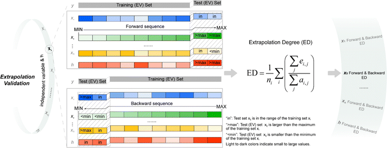

Fig. 1 Schematic of extrapolation degree (ED). h is defined in eqn (9); “forward sequence” means that the samples in the data set are sorted according to the independent variable x_i from the smallest to the largest; “backward sequence” means that the samples in the data set are sorted according to the independent variable x_i from the largest to the smallest; see eqn (10) for the definition of ED.

The leverage value (h) is part of the applicability domain (AD) of the QSPR model.⁴⁷ The AD is defined as the space that contains the chemical space of the molecules in the training set. The AD is both important for model evaluation and recognised by the Organization for Economic Co-operation and Development (OECD).⁴⁸ Within chemistry and drugs among other related fields, h is often used to check compounds affected by structure (i.e., independent variables) in QSPR modeling.⁴⁹h is defined by all independent variables in the model, as described in eqn (9).

h = x_i(X^TX)⁻¹x^T_i (9)

x_i is the independent variable row-vector of the i-th sample, x^T_i is the transpose of x_i, X is the independent variable matrix, and X^T is the transpose of X.

Considering the contribution from all the independent variables, the serialized h is applied for dividing the training and test sets. Both forward serialization (from small to large values) and backward serialization (from large to small values) are adopted, i.e., forward extrapolation validation and backward extrapolation validation. Following this approach, all independent variables for the developed model are evaluated.

To describe the EV method clearly, a list of its steps is as follows:

(1) Calculate the training set sample leverage value (h) according to eqn (9).

(2) Sort the same one independent variable (x_i) for all training set samples from the smallest to the largest (i.e., forward sequence).

(3) The first 80% of the samples in the sorted training set are used as the training (EV) set, and the last 20% of the samples are used as the test (EV) set.

(4) Fitting the developed model using the training (EV) set.

(5) Using the re-fitted model in step 4 to predict the test (EV) set samples, evaluate the performance of the re-fitted model on the test (EV) set.

(6) Repeat steps 2 to 5 for h and all independent variables (x).

(7) Replace the order of the training set samples in step 2 to “follow the order from the largest to the smallest (i.e., backward sequence) of the training set x_i”, and then repeat steps 2 to 6 for h and all x.

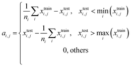
When serializing extrapolation for one independent variable, it is difficult to ensure that all independent variables in the test (EV) set are outside the corresponding range of the training (EV) set, at which point the performance of the test (EV) set will inevitably include the contribution from interpolation. Hence, the extrapolation degree (ED; eqn (10) and Fig. 1) is defined as a metric to assist in evaluating the extrapolation ability of the model. Of those, “e_i,j” in the definition of ED is the distance at which the independent variable i of sample j in the test set is outside the range of independent variable i in the training set. Since not all sample independent variables of the test (EV) set are outside the range of the training set, the performance of the test set (EV) includes the contribution from interpolation ability. The ED quantifies the extent to which the independent variables of the test (EV) set are outside the corresponding domain of definition of the training set, thereby digitizing the fraction of the test (EV) set performance that is really extrapolated. When the performance of the test (EV) set is good and the ED is high, it indicates that the predicted values of the model are reliable even for the samples that are farther away from the training domain. And when the performance of the test (EV) set is good and the ED is low, it indicates that the model may only be able to extrapolate to the samples in the closer range outside the training domain. Therefore, ED can be used as an assistant metric to evaluate the extrapolation ability of a model. Furthermore, the standard deviation of the samples within the 95% confidence level interval (σ₉₅, eqn (S2)†) is presented as a threshold for the evaluation of the extrapolation ability. If the RMSE_test(EV) of an independent variable is greater than σ₉₅, then it is possible that the prediction error of the model is greater than the difference between the actual value and the mean of the samples within the 95% confidence level interval. The average of all RMSEs of the re-fitted models after serialisation of the independent variables and h, i.e. the average RMSE, is taken as a statistical parameter to evaluate the overall extrapolation ability of the model.

where i and j are the serial numbers of the independent variables and samples, respectively, and n_i and n_j are the number of independent variables and samples.

3 Results and discussion

3.1 Results of the mathematical model extrapolation test

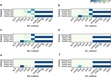
Based on the results of models established for data with deterministic functional relationships with the initial hyperparameters of the 11 ML methods (Fig. 2a–c, ESI Text S2 and Tables S1–S3†), it is found that the regressors involving tree algorithms (i.e., RF, KNN, XGB, AdaBoost, and GBDT) show excellent predictability in the value domain of the training set, which is confirmed by the coefficient of determination (R², eqn (S3)†) of the training set and test (I) set being close to 1. However, facing target values outside the value domain of the training set, their predicted vs. observed values behave as horizontal straight lines, with the fact that R_test(B)² and R_test(F)² are both 0. This suggests that ML models involving tree algorithms have great interpolation ability but may not have extrapolation ability. Since hyperparameters have non-negligible effects on model performance, the hyperparameters of the models established by the 10 methods other than MLR are optimized. Even for the optimal models (Fig. 2d–f and ESI Tables S4–S9†), R_test(B)² and R_test(F)² of the ML models involving tree algorithms are still 0, which rules out the correlation between extrapolation inability and hyperparameter selection. Furthermore, the predicted values of the optimal models of the MLR, LASSO, GPR, and MLP methods are almost close to the observed values. Nevertheless, Ridge and SVM models using data from linear or nonlinear multivariate functional relationships have large prediction errors when observed values are far away from the domain of values in the training set, as evidenced by their R_test(B)² failing to reach 1 (Fig. 3e and f).

Fig. 2 Predicted values vs. observed values for the training set, test (F) set, test (I) set, and test (B) set of the initial hyperparametric model established for data with deterministic functional relationships, i.e., (a) linear univariate, (b) linear multivariate, and (c) nonlinear multivariate, by 11 ML methods; predicted values vs. observed values for the training set, test (F) set, test (I) set and test (B) set of the optimal hyperparametric model established for data with deterministic functional relationships, i.e., (d) linear univariate, (e) linear multivariate, and (f) nonlinear multivariate, by 11 ML methods.

Fig. 3 R ² for the training set, test (F) set, test (I) set, and test (B) set of the initial hyperparametric model established for data with deterministic functional relationships, i.e., (a) linear univariate, (b) linear multivariate, and (c) nonlinear multivariate, by 11 ML methods; R² for the training set, test (F) set, test (I) set and test (B) set of the optimal hyperparametric model established for data with deterministic functional relationships, i.e., (d) linear univariate, (e) linear multivariate, and (f) nonlinear multivariate, by 11 ML methods.

During hyperparameter conditioning of the regressors involving tree-based algorithms (ESI Fig. S1–S3†), all predictions in the test (B) and test (F) sets are close to the maximum and minimum values in the training set, respectively. Particularly noteworthy is that AdaBoost, RF, and XGBoost models exhibit piecewise functional data relationships as the hyperparameters are varied, therefore, conjecturing that this may be the reason for the extrapolation-failure of the model developed by ML methods involving tree algorithms, i.e., having constant output values for a certain range of input values.

Furthermore, for samples far from the domain of definition of the training set, the predicted values of Ridge and SVM models developed with linear or nonlinear multivariate functional relationship data differ significantly from their observed values (Fig. 2e and f). This emphasizes the fact that the reliability of the predicted values of a model for dataset out-of-distribution samples is related to the distance between the sample independent variable and the domain of definition of the training set. If the ED in the EV is small (i.e., the extrapolation ability contributes less) and the extrapolation ability is worse (i.e., the performance of the test (EV) set is worse), while the ED of the predicted sample is large, one can consider the reliability of the model predicted values to be low in this case.

3.2 Reasons for the difficulty of discovering new materials & chemicals via ML models involving tree algorithms

To gain insights into the reason for the poor extrapolation ability of regressors involving tree algorithms, an RF model developed for data from the linear univariate functional relationship is visualized, which contains 10 Decision Trees (DTs), each of depth 4 (Fig. 4, ESI S4 and S5†). Each node can be considered as a dichotomy point in the decision-making process. For any input value lower than the domain of the definition of the training set, each node is determined to be “True”, so the predicted value of each DT is the minimum of its value domain. For any input value higher than the domain of the definition of the training set, each node is determined to be “False”, so the predicted value of each DT is the maximum of its value domain. The predicted value of the RF model is the average of the predicted values of all DTs. The example model, with only one independent variable, has a maximum predictive value of 979.9619 and a minimum predictive value of 417.0969, the potential predicted value range is [417.0969, 979.9619] (ESI Fig. S4†). Thus, the range of potential predicted values for any of the independent variables is a closed interval in the case of ML methods involving tree algorithms.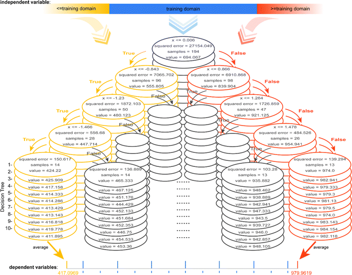

Fig. 4 Schematic diagram of the model architecture containing 10 DTs (each with a depth of 4) for data with linear univariate relationships via the RF method.

When having multiple independent variables, the dependent variable is a combined transformation of values within these closed intervals. Furthermore, the value domain constituted by the combined transformations of the potential maximum to minimum predicted values of all the independent variables is a closed interval, which may be the reason for extrapolation-failure of the models developed by ML methods involving tree algorithms. It should be noted that because the regression models involving tree algorithms have low extrapolation ability, they may have difficulty discovering novel materials or chemicals.

3.3 Application of the EV method for mathematical models

Adopting the EV method, the optimal models for the tested data of three mathematical relationships are evaluated (Fig. 5a–c, ESI S6, S7 and Text S3†). Root mean squared error (RMSE, eqn (S4)†) is adopted as the main statistical parameter in this work. For distinction, the RMSEs on the test (EV) set for the developed model and the model re-fitted by the training (EV) set are represented by RMSE_test(model) and RMSE_test(EV). For the data from whether linear or nonlinear relationships, RMSE_test(EV) of models developed by methods involving tree algorithms, such as AdaBoost, RF, and GBDT, is large. For example, RMSE_test(EV) of ML models involving tree algorithms developed on the data obtained from linear univariate functions were all greater than 50 (Fig. 5a). Models established by methods such as MLP, GPR, and SVM have better extrapolation ability, i.e., RMSE_test(EV) is nearly 0. Results of EV indicate that the models developed by ML methods involving tree algorithms have poor extrapolation ability, while the models developed by ML methods not involving tree algorithms have good extrapolation ability, which is consistent with the results of Section 3.1. Furthermore, since the methods involving tree algorithms have small prediction errors in model development (i.e., RMSE_test(model)) but big prediction errors in the model application (i.e., RMSE_test(EV)), this creates the phenomenon of performance degradation leading to reduced ML model trust. So, a prior evaluation of extrapolation ability using the EV method will help in selecting a trustworthy ML model.

Fig. 5 Results of extrapolation validation (EV) for the ML model developed with data from (a) linear univariate, (b) linear multivariate, and (c) nonlinear multivariate relationships.

3.4 Application of the EV method for the PI-T_g model

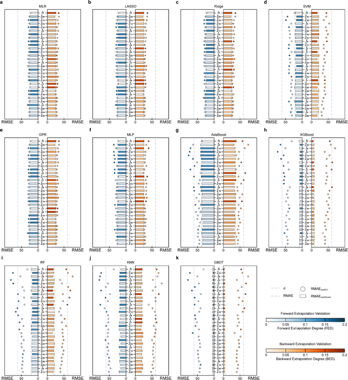
An application of the EV method is demonstrated with the help of a PI model,⁵⁰ developed on a dataset containing 1321 T_g. In previous work, after external validation and leave-one-out cross-validation, the established multiple linear regression (MLR) model containing 29 descriptors was sufficient to ensure predictive accuracy and robustness, i.e., R_testing² and Q² of 0.8793 and 0.8718, respectively. Besides the MLR model developed in the literature, 10 models such as MLP, RF, and GBDT are established, all of which are fully consistent with the literature in terms of independent variables (norm index, I), training set, and test set settings (ESI Text S4, Table S10 and Fig. S8†). The extrapolation ability of 11 PI-T_g models is evaluated by the EV method (Fig. 6, 7 and ESI Text S5†).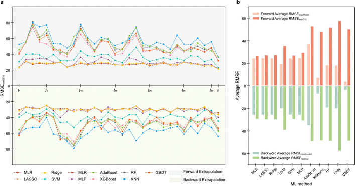

Fig. 6 11 PI-T_g model extrapolation validation (EV): (a) overall result and (b) average RMSE statistical value.

Fig. 7 Extrapolation validation (EV) results of (a) MLR, (b) LASSO, (c) Ridge, (d) SVM, (e) GPR, (f) MLP, (g) AdaBoost, (h) XGBoost, (i) RF, (j) KNN and (k) GBDT model. Note: the top-to-bottom order of the independent variables in the EV result plots is consistent with the large-to-small order of the sum of the differences between RMSE_test(EV) and RMSE_test(model) of the forward extrapolation validation and backward extrapolation validation.

In the case of EV instance for PI-T_g models, the RMSE_test(EV) for forward and backward serialized extrapolation validations for models established by the involving tree algorithm is always larger than that for models established by the non-tree-involving algorithm, for every I and h (Fig. 6a). To evaluate the overall extrapolation ability of the model, the average of RMSE for the all independent variable and h extrapolation validation, i.e., the average RMSE_test(EV) and the average RMSE_test(model), is used as the statistical parameter. The average RMSE_test(EV) of MLP, MLR, Ridge, GPR, and LASSO is around 20 °C (Fig. 6b), which is close to the experimental measurement error and acceptable.⁵¹ By contrast, the average RMSE_test(EV) of the models developed based on RF, KNN, GBDT, XGBoost, and AdaBoost methods is larger, with around 40 °C (Fig. 6b), which suggests that these models involving tree algorithms have relatively poor extrapolation ability.

Furthermore, σ₉₅ is presented as a threshold for the evaluation of the extrapolation ability. If the RMSE_test(EV) of an independent variable is greater than σ₉₅, then the prediction error of the model may be greater than the difference between the actual value and the mean of the samples within the 95% confidence level interval. The RMSE_test(EV)s of the ML methods established by involving tree algorithm are generally high, and with several RMSE_test(EV)s are even near the σ₉₅ (60.35 °C; Fig. 7f–j), for instance, the results of the AdaBoost model of forward extrapolation validation with I₁₀, I₁₈, I₃, and I₅ and the backward extrapolation validation of I₉, and I₈ (Fig. 7f), the XGBoost model of I₁₀ and I₃ forward serialization extrapolation and I₉ backward serialization extrapolation (Fig. 7g). This indicates that the prediction error of this model even exceeds AE when the above-mentioned independent variable in the sample exists far away from the corresponding domain of definition of the training set.

The MLP, MLR, LASSO, GPR, and Ridge models have RMSE_test(EV) of any I close to the corresponding RMSE_test(model) (Fig. 7a–e), which indicates their good predictive ability. Furthermore, I₁₀, I₁₃, and I₉ of the SVM model have small backward EDs along with large RMSE_test(EV), therefore, in applying this model, if there are I₁₀, I₁₃, and I₉ in the prediction samples that are smaller than the minimum in the corresponding training set, the predicted values may be unreliable, i.e., extrapolation of such an independent variable is not recommended. In contrast, the I₅ in the SVM model has a high forward ED but a small RMSE_test(EV). It means that this independent variable has little effect on the prediction reliability of the model when it exceeds the definitional domain of the corresponding training set, therefore, the predicted value of the sample can be considered reliable when such independent variables are extrapolated.

4 Conclusions

In this contribution, the extrapolation ability of models established by multiple ML methods is explored. Furthermore, the extrapolation validation (EV) method is proposed to quantitatively evaluate the extrapolation ability of a model. Establishing ML models from data with deterministic functional relationships found that ML models involving tree algorithms are fixed for predicted values out of the training set domain, confirming its extrapolation-failure phenomenon. Taking the RF model as an example reveals that the intrinsic reason for the poor extrapolation ability of the regressor involving tree algorithms may be that the value domain constituted by the combined transformations of the potential maximum to minimum predicted values of all the independent variables is a closed interval. The EV validation results for the ML model with the data from defined functional relationships and with the 1321 PI-T_g data confirm that the models developed by ML methods involving tree algorithms have poor extrapolation ability, while the models developed by ML methods not involving tree algorithms have good extrapolation ability. Before transitioning a model to applications, the EV method is sufficient to evaluate the extrapolation ability of the model and help in selecting trustworthy ML models. Meanwhile, the ED gives digital advice on the extent of reliability for the models to predict samples.

The EV method is independent of the architecture of the developed model. Essentially, the EV method is a pioneering dataset division scheme that is based on the range of each independent variable/descriptor/dimension in the training set. It evaluates the extrapolation of each variable by serializing each independent variable (i.e., sorting from the smallest to the largest and from the largest to the smallest) and later dividing the training and test sets. Some predictive models developed based on ML architectures such as advanced generative adversarial network (GAN), convolution neural network (CNN), and recurrent neural network (RNN) can be considered for evaluating the extrapolation ability of the models via the EV method. Meanwhile, it provides the Data Science community with some insights and solutions for evaluating the reliability of out-of-distribution sample prediction in ML models (e.g., molecular and material properties, reaction yields, etc.).

Data availability

The data for the three mathematical relationship models obtained in this work have been provided in the ESI.† The 1321 polyimide (PI) glass transition temperature (T_g) dataset is available from https://pubs.acs.org/10.1021/acs.jcim.2c01389. The 33 mathematical relationship ML models developed in this paper and the 10 PI-T_g models are available from GitHub (https://github.com/fangyouyan). Example code for the extrapolation validation (EV) method can be viewed from GitHub (https://github.com/fangyouyan). The 11 machine learning (ML) algorithm models were developed using the scikit-learn⁵² package version 1.3.0 in Python⁵³ 3.11 and the xgboost⁵⁴ package version 1.7.6. The models were accessed via the joblib⁵⁵ package version 1.2.0. Random forest (RF) models were visualized with Pydotplus package version 2.0.2.

Author contributions

M. X. Y. conceived the problem and carried out all detailed studies. F. Y. Y. analysed the problem and designed the method. M. X. Y., F. Y. Y., and Y. N. Z. co-analysed the results. M. X. Y. wrote the manuscript, F. Y. Y. and Y. N. Z. made modifications. Q. W. provided strategic guidance. All authors contributed to useful discussions.

Conflicts of interest

There are no conflicts to declare.

Acknowledgements

This work was financially supported by the National Natural Science Foundation of China (22278319 and 22222807).

Notes and references

1. D. Doudesis, K. K. Lee, J. Boeddinghaus, A. Bularga, A. V. Ferry, C. Tuck, M. T. H. Lowry, P. Lopez-Ayala, T. Nestelberger, L. Koechlin, M. O. Bernabeu, L. Neubeck, A. Anand, K. Schulz, F. S. Apple, W. Parsonage, J. H. Greenslade, L. Cullen, J. W. Pickering, M. P. Than, A. Gray, C. Mueller, N. L. Mills and CoDE-ACS Investigators, Nat. Med., 2023, 29, 1201–1210.
2. E. C. Fricke, C. Hsieh, O. Middleton, D. Gorczynski, C. D. Cappello, O. Sanisidro, J. Rowan, J.-C. Svenning and L. Beaudro, Science, 2022, 377, 1008–1011.
3. N. Ratledge, G. Cadamuro, B. de la Cuesta, M. Stigler and M. Burke, Nature, 2022, 611, 491–495.
4. J. Jiménez-Luna, F. Grisoni and G. Schneider, Nat. Mach. Intell., 2020, 2, 573–584.
5. E. So, F. Yu, B. Wang and B. Haibe-Kains, Nat. Mach. Intell., 2023, 5, 792–798.
6. J. Yang, A. A. S. Soltan, D. W. Eyre and D. A. Clifton, Nat. Mach. Intell., 2023, 5, 884–894.
7. J. Bures and I. Larrosa, Nature, 2023, 613, 689–695.
8. R. Batra, L. Song and R. Ramprasad, Nat. Rev. Mater., 2020, 6, 655–678.
9. Z. Rao, P.-Y. Tung, R. Xie, Y. Wei, H. Zhang, A. Ferrari, T. P. C. Klaver, F. Körmann, P. T. Sukumar, A. K. d. Silva, Y. Chen, Z. Li, D. Ponge, J. Neugebauer, O. Gutfleisch, S. Bauer and D. Raabe, Science, 2022, 378, 78–85.
10. L.-C. Xu, J. Frey, X. Hou, S.-Q. Zhang, Y.-Y. Li, J. C. A. Oliveira, S.-W. Li, L. Ackermann and X. Hong, Nat. Synth., 2023, 2, 321–330.
11. X. Wang, Z. Li, M. Jiang, S. Wang, S. Zhang and Z. Wei, J. Chem. Inf. Model., 2019, 59, 3817–3828.
12. M. R. Dobbelaere, Y. Ureel, F. H. Vermeire, L. Tomme, C. V. Stevens and K. M. Van Geem, Ind. Eng. Chem. Res., 2022, 61, 8581–8594.
13. F. H. Vermeire, Y. Chung and W. H. Green, J. Am. Chem. Soc., 2022, 144, 10785–10797.
14. K. Yang, K. Swanson, W. Jin, C. Coley, P. Eiden, H. Gao, A. Guzman-Perez, T. Hopper, B. Kelley, M. Mathea, A. Palmer, V. Settels, T. Jaakkola, K. Jensen and R. Barzilay, J. Chem. Inf. Model., 2019, 59, 3370–3388.
15. X. Zhu, V. R. Polyakov, K. Bajjuri, H. Hu, A. Maderna, C. A. Tovee and S. C. Ward, J. Chem. Inf. Model., 2023, 63, 2948–2959.
16. M. Zaslavskiy, S. Jégou, E. W. Tramel and G. Wainrib, Comput. Toxicol., 2019, 10, 81–88.
17. J. Ferraz-Caetano, F. Teixeira and M. N. D. S. Cordeiro, J. Chem. Inf. Model., 2024, 64, 2250–2262.
18. P. Li, Y. Li, C.-Y. Hsieh, S. Zhang, X. Liu, H. Liu, S. Song and X. Yao, Briefings Bioinf., 2021, 22, 1–10.
19. Y. Peng, J. Wang, Z. Wu, L. Zheng, B. Wang, G. Liu, W. Li and Y. Tang, Digital Discovery, 2022, 1, 115–126.
20. S. Back, A. Aspuru-Guzik, M. Ceriotti, G. Gryn’ova, B. Grzybowski, G. H. Gu, J. Hein, K. Hippalgaonkar, R. Hormázabal, Y. Jung, S. Kim, W. Y. Kim, S. M. Moosavi, J. Noh, C. Park, J. Schrier, P. Schwaller, K. Tsuda, T. Vegge, O. A. von Lilienfeld and A. Walsh, Digital Discovery, 2024, 3, 23–33.
21. Y. Wang, C. Pang, Y. Wang, J. Jin, J. Zhang, X. Zeng, R. Su, Q. Zou and L. Wei, Nat. Commun., 2023, 14, 6155.
22. S. Chen and Y. Jung, JACS Au, 2021, 1, 1612–1620.
23. C. W. Coley, L. Rogers, W. H. Green and K. F. Jensen, ACS Cent. Sci., 2017, 3, 1237–1245.
24. H. Plommer, I. O. Betinol, T. Dupree, M. Roggen and J. P. Reid, Digital Discovery, 2024, 3, 155–162.
25. O.-H. Choung, R. Vianello, M. Segler, N. Stiefl and J. Jiménez-Luna, Nat. Commun., 2023, 14, 6561.
26. A. Hagg and K. N. Kirschner, J. Chem. Inf. Model., 2023, 63, 4505–4532.
27. P.-Y. Kao, Y.-C. Yang, W.-Y. Chiang, J.-Y. Hsiao, Y. Cao, A. Aliper, F. Ren, A. Aspuru-Guzik, A. Zhavoronkov, M.-H. Hsieh and Y.-C. Lin, J. Chem. Inf. Model., 2023, 63, 3307–3318.
28. E. Heid, C. J. McGill, F. H. Vermeire and W. H. Green, J. Chem. Inf. Model., 2023, 63, 4012–4029.
29. H. Harb, S. N. Elliott, L. Ward, I. T. Foster, S. J. Klippenstein, L. A. Curtiss and R. S. Assary, Digital Discovery, 2023, 2, 1813–1830.
30. H. S. Stein, Trends chem., 2022, 4, 682–684.
31. B. Eshete, Science, 2021, 373, 743–744.
32. J. A. Keith, V. Vassilev-Galindo, B. Cheng, S. Chmiela, M. Gastegger, K. R. Muller and A. Tkatchenko, Chem. Rev., 2021, 121, 9816–9872.
33. E. S. Muckley, J. E. Saal, B. Meredig, C. S. Roper and J. H. Martin, Digital Discovery, 2023, 2, 1425–1435.
34. A. Bender, N. Schneider, M. Segler, W. Patrick Walters, O. Engkvist and T. Rodrigues, Nat. Rev. Chem, 2022, 6, 428–442.
35. K. Li, B. DeCost, K. Choudhary, M. Greenwood and J. Hattrick-Simpers, npj Comput. Mater., 2023, 9, 55.
36. R. Balestriero, J. Pesenti and Y. LeCun, arXiv, 2021, preprint, arXiv:2110.09485,  DOI:10.48550/arXiv.2110.09485.
37. P. Raghavan, B. C. Haas, M. E. Ruos, J. Schleinitz, A. G. Doyle, S. E. Reisman, M. S. Sigman and C. W. Coley, ACS Cent. Sci., 2023, 9, 2196–2204.
38. Z. Zhang, A. Sangion, S. Wang, T. Gouin, T. Brown, J. A. Arnot and L. Li, Environ. Sci. Technol., 2024, 58, 3386–3398.
39. M. Toplak, R. Mocnik, M. Polajnar, Z. Bosnic, L. Carlsson, C. Hasselgren, J. Demšar, S. Boyer, B. Zupan and J. Stålring, J. Chem. Inf. Model., 2014, 54, 431–441.
40. N. Mathai, Y. Chen and J. Kirchmair, Briefings Bioinf., 2020, 21, 791–802.
41. J. B. Mitchell, Wiley Interdiscip. Rev.: Comput. Mol. Sci., 2014, 4, 468–481.
42. L. H. Rieger, E. Flores, K. F. Nielsen, P. Norby, E. Ayerbe, O. Winther, T. Vegge and A. Bhowmik, Digital Discovery, 2023, 2, 112–122.
43. R. P. Sheridan, J. Chem. Inf. Model., 2013, 53, 783–790.
44. B. Meredig, E. Antono, C. Church, M. Hutchinson, J. Ling, S. Paradiso, B. Blaiszik, I. Foster, B. Gibbons, J. Hattrick-Simpers, A. Mehta and L. Ward, Mol. Syst. Des. Eng., 2018, 3, 819–825.
45. Z. Xiong, Y. Cui, Z. Liu, Y. Zhao, M. Hu and J. Hu, Comput. Mater. Sci., 2020, 171, 109203.
46. S. Kearnes, Trends Chem., 2021, 3, 77–79.
47. K. Roy, S. Kar and R. N. Das, Understanding the basics of QSAR for applications in pharmaceutical sciences and risk assessment, Academic Press, 2015.
48. P. Gramatica, QSAR Comb. Sci., 2007, 26, 694–701.
49. L. Fu, L. Liu, Z.-J. Yang, P. Li, J.-J. Ding, Y.-H. Yun, A.-P. Lu, T.-J. Hou and D.-S. Cao, J. Chem. Inf. Model., 2019, 60, 63–76.
50. M. Yu, Y. Shi, Q. Jia, Q. Wang, Z. H. Luo, F. Yan and Y. N. Zhou, J. Chem. Inf. Model., 2023, 63, 1177–1187.
51. G. H. Lee, H. Moon, H. Kim, G. H. Lee, W. Kwon, S. Yoo, D. Myung, S. H. Yun, Z. Bao and S. K. Hahn, Nat. Rev. Mater., 2020, 5, 149–165.
52. Scikit-learn, https://scikit-learn.org/stable/.
53. Python, https://www.python.org/.
54. xgboost, https://xgboost.readthedocs.io/en/stable/.
55. joblib, https://joblib.readthedocs.io/en/stable/.

---

Footnote

† Electronic supplementary information (ESI) available. See DOI: https://doi.org/10.1039/d3dd00256j

---