Accelerating metal–organic framework discovery via synthesisability prediction: the MFD evaluation method for one-class classification models

Abstract

Machine learning has found wide application in the materials field, particularly in discovering structure–property relationships. However, its potential in predicting synthetic accessibility of materials remains relatively unexplored due to the lack of negative data. In this study, we employ several one-class classification (OCC) approaches to accelerate the development of novel metal–organic framework materials by predicting their synthesisability. The evaluation of OCC model performance poses challenges, as traditional evaluation metrics are not applicable when dealing with a single type of data. To overcome this limitation, we introduce a quantitative approach, the maximum fraction difference (MFD) method, to assess and compare model performance, as well as determine optimal thresholds for effectively distinguishing between positives and negatives. A DeepSVDD model with superior predictive capability is proposed. By combining assessment of synthetic viability with porosity prediction models, a list of 3453 unreported combinations is generated and characterised by predictions of high synthesisability and large pore size. The MFD methodology proposed in this study is intended to provide an effective complementary assessment method for addressing the inherent challenges in evaluating OCC models. The research process, developed models, and predicted results of this study are aimed at helping prioritisation of materials for synthesis.

---

Introduction

Traditional binary classification problems are typically characterised as supervised learning tasks focusing on distinguishing between two well-represented classes. Nevertheless, building traditional classifiers becomes challenging when one of the classes is significantly underrepresented. One-class classification (OCC) is applicable in such cases. It aims to build a model of a single normal class, and to identify instances that do not conform to this normal class as anomalies based exclusively on the information from this normal category. OCC plays a critical role in various practical applications, including domains such as cybersecurity, quality control, and fault detection.^1,2 However, its utilisation in material discovery and research has been relatively limited. This limitation can be attributed to several factors. Firstly, materials science problems often involve multi-class problems, particularly in the field of property prediction. Secondly, the intricate nature and characteristics of materials add an extra layer of complexity, rendering the application of classification models even more challenging. Most importantly, while OCC models require only one class of data for training (e.g. the composition of materials which can be synthesised), it is still essential to include samples which lie outside of this class for validation (e.g. compositions where materials cannot be synthesised). In materials research, obtaining negative samples are particularly difficult due to the intricacies of the experimental and testing process, and the tendency not to report “failed” synthetic experiments in literature. Therefore, an inherent challenge posed by such OCC problems characterised by the paucity of negative samples for both training and validation lies in evaluating the performance of machine learning (ML) models, as conventional evaluation metrics cannot be applied.

Typically, the performance of a classification model is assessed by calculating various indicators including accuracy, precision, recall, F1 score, receiver operating characteristic (ROC) curve, and area under curve (AUC) based on four entries of the predictions made by a model in comparison to the actual labels of the data, i.e., true positives (TP), false positives (FP), true negatives (TN), and false negatives (FN). However, in the case of one-class classification, only the TP and FN can be obtained since only “true” actual values are available. Consequently, only the true positive rate (TPR), also referred to as recall or sensitivity, can be calculated. Relying solely on the TPR is insufficient for a comprehensive evaluation of a model's quality as a perfect TPR of 1 is consistently attainable if a model predicts everything as “positive” and does not attempt to differentiate between positive and negative samples. To address this issue, we present a quantitative approach, the maximum fraction difference (MFD) method, which enables the evaluation of model performance for the task of training an OCC model to differentiate between negative and positive samples and thus predict the instances of an unknown dataset that are most likely to belong to the positive labelled class. The MFD method then facilitates a comparative analysis among different OCC models without the need of negative data for validation. The MFD method allows a distinct classification threshold to be selected for each trained model to attain improved predictive performance which is based on the anomaly score predictions generated by various OCC models. We exemplify the MFD method here by training and evaluating OCC models for the task of predicting the synthesisability of metal–organic frameworks (MOFs).

MOFs, also known as porous coordination polymers, are hybrid porous materials with one-, two-, or three-dimensional structures formed by the self-assembly of organic ligands and metal ions/clusters through coordination bonds. Since the late 1990s, when MOFs with stable and robust frameworks were discovered, pioneering work in the development of MOFs has made them a well-suited and popular approach in many different fields, such as energy and medicine.^3–8 Compared with other nanoporous materials, MOFs are typically characterised by high porosity, large specific surface area, tuneable structure, and ease of functionalization.⁹

The properties of MOFs arise from the combination of the component building units: metal centres and organic linkers. Metal ions or clusters form the central building blocks of MOF structures, imparting rigidity and stability to the coordination network with specific structures and properties.¹⁰ Organic linkers, the other essential building units that serve as bridges, can be adjusted to modulate functionalities such as pore size, chemical reactivity and adsorption selectivity of materials.^11,12 By purposeful selection of metal centres and organic linkers, MOFs with controllable pore structure, higher stability and modifiable active sites can be designed to meet specific application requirements.

The philosophy of molecular design driven by framework design principles outlined for MOFs has been used to facilitate new materials discovery with great success. A number of crystalline MOFs with preferred topologies are formed by “reticular synthesis”, a conceptual approach assembling judiciously designed molecular building blocks into predetermined rigid and ordered frameworks, which creates strong coordination bonds between inorganic and organic units.^11,13 However, the successful synthesis of a wider range of MOFs with distinct crystal and pore structures that conform to desired design specifications and exhibit expected physical and chemical characteristics remains a process of “trial-and-error” informed by chemical understanding and expert knowledge. Developments in high-throughput experimental techniques and computational screening approaches^14–16 have enabled the synthesis and evaluation of a much larger number of materials. The integration of data science techniques, particularly those based on ML workflows, with experimental discovery offers a new direction in material research. It allows systematic material data evaluation at scale to offer statistical advice and concurrently assist chemists in discerning and prioritizing certain chemistries when designing new materials.^6,17 ML can numerically represent real chemical problems and address complex issues, particularly those involving large combinatorial spaces, non-linear processes, or problems that cannot be precisely modelled by existing theoretical methods.^18,19 For instance, it can be used to analyse potential relationships between the high-temperature/solvent-removal stability of MOFs and their chemical/geometric structures,²⁰ and also to accelerate the discovery of low thermal conductivity oxides²¹ or high-performance inorganic crystalline solid-state lithium ion (Li⁺) electrolytes.^22,23

To date, over 100 000 experimental MOF structures have been synthesised and deposited into the Cambridge Structural Database (CSD).²⁴ Alongside these experimentally synthesised MOFs, a substantially larger number of hypothetical MOFs²⁵ have been generated computationally to identify the most promising materials for a desired application by systematically traversing feasible combinations of building units in diverse topologies. However, these are still only a small part of the overall MOF potential design space. The richness of this space is attributed to the extensive selection of metal atoms available, combined with a virtually infinite choice of organic counter parts.²⁶ It is informative to contrast MOFs with another type of porous materials, zeolites, for which only 255 structures have been realised experimentally but over 300 000 hypothetical structures have been proposed. Such imbalance between the positive and unlabelled datasets makes it reasonable to consider the hypothetical dataset as negative samples.²⁷ This approximation allows the application of common classification methods and the use of common model performance metrics and is a basis of positive-unlabelled or PU learning also used in other synthesisability prediction tools^28–31 when the number of proposed hypothetical materials is very large and the success rate in synthesising materials has been relatively slow. This assumption may not hold for MOF synthesis where discovery of new materials is very rapid, and so we instead apply the formalism of the one class classifier (OCC) model.

In recent research, OCC has proven effective in the synthesis of co-crystals³² and the discovery of crystalline inorganic solids.²³ Here, we test several different algorithms for OCC and implement the MFD method to select well-performing models that can provide guidance on the probable synthetic accessibility of MOF materials composed of one metal and a single linker, thus expediting the development of novel MOF materials for different applications. The ground-truth data used in this study is obtained from Pétuya et al.’s work³³ on predicting the guest accessibility of MOFs. This dataset was built from 3D-connected MOF networks made of a single metal and a single linker species in the CSD MOF subset. It was therefore referred to as the 1M1L3D dataset. The available ground-truth data are restricted to a single class of successful synthetic attempts, while negative data from unsuccessful synthetic attempts are comparatively lacking in scale. Under the condition of having extremely unbalanced dataset, OCC is well-suited to discerning the underlying relationships between composition and synthesisability. Taking all of the separate metals and linkers contained in the 1M1L3D dataset, we then generate a larger query dataset of 160 582 potential MOF chemistries by considering every pairwise combination of these metals and linkers that are not contained in the 1M1L3D dataset.

The performance of ML models developed in the field of materials can be influenced by several factors, including the training data, representations used, and the choice of algorithms. In this study, we comprehensively evaluate a diverse range of features to effectively represent materials for the synthesisability problem, including three different sets of metal features and three distinct groups of linker features, as shown in Fig. 1. Various OCC algorithms are examined, encompassing five well-established classic approaches as well as two advanced neural network-based methods. Ultimately, the MFD is proved to be an effective metric to assess the performance of OCC models. We report a deep-learning based model with superior capability to predict the likelihood whether a MOF can be synthesised given a combination of any single metal and single linker. This model correctly predicts that 12 of 14 unseen negative samples cannot be synthesised. The synthesisability prediction using the best-performing model and the porosity prediction using random forest sequential models³³ are conducted concurrently on the query dataset. Out of the entire set of 160 582 metal and linker combinations, 3453 are predicted to be synthesisable and to have a high pore limiting diameter (PLD), indicating their higher probability of providing a large guest-accessible space and being successfully synthesised.

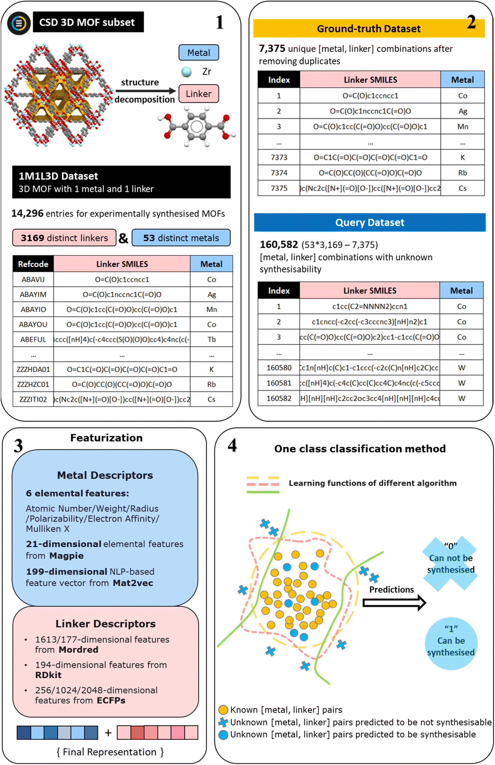Fig. 1 The workflow for dataset creation, feature generation, and model training. The starting point is the 1M1L3D dataset³³ previously derived from the CSD MOF subset (step 1). Then the positively ground-truth dataset is created from distinct metal and distinct linker combinations by removing duplicate combinations in 1M1L3D dataset. The query dataset contains the remaining [metal, linker] combinations not present in the 1M1L3D dataset (step 2). Three sets of metal features and three groups of linker features are generated (step 3) to train one-class classification models predicting MOFs synthesisability (step 4).

Methods

Datasets

The 1M1L3D dataset used to train models is obtained from Pétuya et al.³³ This dataset is sourced from decomposing reported experimental three-dimensional MOF structures made of a single metal and a single linker in CSD into their constituent components, expressed as metal symbols and canonical simplified molecular input line-entry (SMILES) strings. As shown in Fig. 1 (steps 1–2), the 1M1L3D dataset consists of 14 296 MOFs with unique refcodes (entries) in total. Among these data, there are 6921 duplicated [metal, linker] combinations with multiple CSD entries. In this case, 7375 unique [metal, linker] pairs remained that are known to produce MOFs and can be directly used for model training, denoted as the “Ground-truth” dataset. Any combination of metal ions/clusters and organic ligands can be attempted to synthesise a MOF structure. For this study, we exclusively use metal ions/clusters and organic ligands from the reported structures to generate a query set. Thus, the dataset encompasses 53 distinct metals and 3169 distinct linkers, resulting in 53 × 3169 = 167 957 possible [metal, linker] combinations. Only 7375 of them have been reported to produce MOFs. By training our model on these “ground-truth” positive examples, we can identify the most promising [metal, linker] combinations from the remaining 160 582 possibilities (also denoted as the “Query” dataset).

To assess the performance of our best model in correctly reporting [metal, linker] combinations which are known not to form MOFs, we select a small dataset of negative samples by combining eight samples that did not yield a MOF despite being extensively studied in our group and six [metal, linker] combinations taken from the study conducted by Banerjee et al.³⁴ focusing on the high-throughput synthesis of ZIFs via 9600 micro-reactions involving combinations of zinc(II)/cobalt(II) and nine different imidazolate/imidazolate-type linkers. In the field of materials synthesis, a significant obstacle in attaining negative samples with certainty lies in the potential ambiguity surrounding synthesis failures. While it is difficult to definitively assert the impossibility of synthesising a MOF using the given [metal, linker] combination under all possible conditions, unsuccessful synthesis attempts for these 14 combinations still indicate that the researchers invested considerable effort (30–50 attempted reactions performed by an expert chemist for each combination) but no MOF was produced. We take [‘Zr’, ‘O=C(O)CNC(=O)c1ccc(C(=O)NCC(=O)O)cc1’] from the set of negative combinations as an example that shows (Table S1†) the typical experimental attempts invested to deem this combination as unable to produce a MOF.

Descriptors

In the field of materials informatics, featurization schemes describing materials as component vectors are common, with the aim of using ML to predict their properties. Choosing the approach transforming raw materials data into the quantitative descriptions, i.e., the features, is one of the key steps to build an accurate model. As shown in Fig. 1 (step 3), in this work, we utilise three different features to represent the metal in the MOF. First, we select 6 elemental descriptors that were consistently identified as important features in the MOF porosity prediction model developed by Pétuya et al.,³³ with an accuracy of 80.5%, from which we obtained the ground-truth dataset. In addition, 21-dimensional elemental descriptors from magpie³⁵ and 199-dimensional natural language processing (NLP)-based descriptors from mat2vec³⁶ are also considered. Magpie is an example of the composition-based feature vector (CBFV),^35,37 which is a main philosophy of feature generation in ML-assisted inorganic material design. It is domain-derived and represents materials based on expertly curated element properties. Moreover, it is human-readable, and potentially capable of physical interpretation. In this study, only 21 elemental descriptors are used for the metal species. Contrary to the CBFV are data-driven techniques, of which mat2vec serves as a prototype. In this method, material science knowledge is encoded as information-dense word embeddings that capture complex materials science concepts and relationships.

Regarding the featurization of linkers, we tried three commonly used approaches: Mordred,³⁸ RDkit,³⁹ and extended-connectivity fingerprints (ECFPs).^40,41 Mordred is a freely available Python-based molecular descriptor calculator that provides access to 1613 pre-defined 2D molecular descriptors. It is widely used in cheminformatics research and has proven to have good performance. RDkit is an open-source cheminformatics software toolkit that also allows for the generation of over 200 molecular descriptors based on various molecular properties. Following the elimination of feature columns containing only zeros, a total of 194 descriptors remained for further analysis. ECFPs, an example of circular fingerprints that represent a class of hashed fingerprints for molecular characterisation, encode the substructure of a molecule using a circular algorithm, exhibiting a distinct principle from the other two methods. The generation process includes two main stages: an initial assignment stage in which each atom has an integer identifier assigned to it, and an iterative updating stage in which each atom identifier is updated to reflect the identifiers of their neighbours. In the final step, the identifiers will be hashed into and stored as a variable-length list of “on” bits. The selection of two key hyperparameters, “radius” and “bits”, is in turn essential for the aforementioned processes. The “bits” parameter determines the number of bits in each fingerprint, and can be adjusted to regulate the sparsity and information content of the fingerprint while mitigating information collapse, i.e., the same feature represents a different substructure. The “radius” parameter controls the number of iterations performed, and hence determines the distance around each atom up to which the fingerprint is generated. In this study, three sizes of fingerprints are generated and evaluated: 256 bits, 1024 bits, and 2048 bits. Furthermore, the “radius” parameter is explored within the range of 2 to 5.

One class classification models

OCC algorithms typically rely on statistical methods or distance metrics, such as the traditional density-based local outlier factor (LOF)⁴² algorithm, the distance-based k-nearest neighbours (kNN) algorithm, and Gaussian mixture model (GMM) based on statistical methods. LOF, kNN, and GMM are traditional algorithms that determine whether a sample belongs to the single ground-truth class or not directly based on the distribution characteristics or relative distance of the data samples (as shown in Fig. 1 (step 4)). Consequently, these approaches generate outcomes that are more straightforward to interpret and subject to in-depth analysis. Moreover, traditional models often exhibit low computational complexity, making them highly efficient and well-suited for handling small dataset. However, it should be noted that these models have two distinct disadvantages. Firstly, due to their lack of trainable parameters, traditional techniques might not perform well under high-dimensional data or when the distribution varies greatly across different regions in the data space. Secondly, substantial feature selection is often required as a crucial pre-processing step to decrease dimensionality and eliminate redundant and irrelevant features. The primary objective is to mitigate overfitting, which can impact the model's prediction and generalisation capacity. In order to overcome the limitations associated with these two aspects of traditional models, we employ two other neural network-based OCC algorithms.

Learnable unified neighbourhood-based anomaly ranking (LUNAR)⁴³ is one of the neural network-based models adopted in this study. It addresses the first limitation by introducing learnability into local OCC methods, providing the capacity to adapt to diverse data distributions and structures, making it more flexible and expressive in handling complex, non-linear, and high-dimensional data. Compared to traditional local OCC methods, the learnability of LUNAR empowers it to exhibit enhanced robustness across various values of the number of nearest neighbours, k.⁴³ Besides, a pre-defined percentage of samples are generated outside of the ground-truth class from the uniform distribution and subspace perturbation, which are then used to introduce supervision to the unsupervised task. Ultimately, LUNAR constructs a k-NN graph, takes a node's distances to its k nearest neighbours as input to the neural network, and subsequently outputs a weighted distance as the final anomaly score.

Deep learning approaches allow for automatic discovery of valuable representations and simplify complex raw data to form “good” features by building and training deep neural networks. An autoencoder, a specific type of deep neural network, consists of encoder and decoder neural network architectures, where the encoder maps the input data into a compressed representation (also known as a latent representation) and the decoder maps the compressed representation back to the original input space. By training the autoencoder to minimise the reconstruction error between the input and output, the model learns a compressed representation that captures the salient features of the data. As a result, deep learning algorithms do not require the feature selection of traditional approaches and are able to automatically learn and extract useful features to detect anomalies. The deep support vector data description (DeepSVDD) architecture, another neural network used in this paper, is sourced from Ruff et al.⁴⁴ and adapted by Vriza et al.³² to accelerate the discovery of π–π co-crystals. In a similar principle with one-class SVM (OCSVM), the DeepSVDD technique aims to identify a smallest hypersphere that contains all of the samples except for a limited number of outliers. This architecture is a two-step process. The first step, i.e., the pre-training step, is composed by an autoencoder for learning a compact data representation that captures the essential information about the data distribution and maps the input data into a hypersphere region. The second step, i.e., the training step, a feed forward neural network architecture is used to learn the transformation and optimise the centre of hypersphere with the aim of minimising the distance between all data representations and the centre.

Ultimately, seven different algorithms exhibiting good performance in distinguishing between the ground-truth and the query dataset are selected. These algorithms range from classical techniques to state-of-the-art neural network-based OCC methods, including: isolation forest (IForest), kNN, OCSVM, LOF, cluster-based LOF (CBLOF), LUNAR, and DeepSVDD. Subsequent evaluations are conducted to choose the best candidate. Except for DeepSVDD, these models are implemented using PyOD,⁴⁵ a comprehensive and scalable Python library for identifying outliers in multivariate data. The DeepSVDD architecture is implemented by substituting the convolutional autoencoder with the set-transformer autoencoder⁴⁶ in the PyTorch implementation of the original DeepSVDD method.

Since some algorithms we use, for example, kNN and LOF, rely on distance for classification, the prediction accuracy can be improved dramatically by normalising the feature space if the features represent different physical units or come in vastly different scales. Hyperparameters of traditional models are optimised using hyperopt from hyperopt library.⁴⁷

Results

The maximum fraction difference (MFD) method

Raw scores predicted by different fitted models indicate the dissimilarity between input query samples and the ground-truth dataset (here, these are the metal and linker combinations in the 1M1L3D dataset) with low scores representing a high probability that an unknown sample belongs in the positive class. In this study, these scores are multiplied by −1 and normalised within the range of [0,1] so that lower scores indicate metal linker pairs which are unlikely to be synthesisable while scores approaching 1 indicate metal linker pairs which are more likely to be synthesisable. We adopt the hypothesis that in a typical OCC problem, the ground-truth dataset comprises exclusively positive samples, whereas a significant proportion of the query dataset consists of a substantial number of true negatives. Although the identity and number of these true negatives remains unknown preventing training of a binary classifier, assuming their existence enables the development of metrics to assess the performance of OCC models. Making further assumptions about the relationship between the ground truth and query datasets can lead to the treatment of related problems using positive unlabelled learning,⁴⁸ however here we prefer not to make any further assumptions and proceed with OCC.

OCC models trained using the ground-truth dataset containing solely positive samples are expected to assign higher scores on average for the ground-truth data and lower scores for a significant proportion of the query data. Given the task of scoring samples in the query dataset to predict which samples are likely to belong to the ground-truth class, a superior model should result in different distributions of scores for the ground-truth dataset and the query dataset. A score distribution for a poorly discriminating model and a successfully discriminating model are illustrated in Fig. 2(a). A superior model should give lower scores on average to the query samples, resulting in a larger separation between the ground-truth (orange) and query (blue) distribution areas. Ideally, the overlap (grey) between these datasets should be small, allowing the identification of a reliable area with a set of query samples which are confidently predicted to lie within the ground-truth class. An inferior model in which the query and the ground-truth data are given very similar distributions is unhelpful, as it cannot provide confident predictions of which query samples are likely to lie in the ground-truth class. In this case, the model tends to predict everything to be positive and therefore get a TPR close to 1.

Fig. 2 Schematic representation of the principle and definition of maximum fraction difference (MFD). The illustration displays a model with poor discrimination (left) and a model with successful discrimination (right). (a) Normalised score distributions of the ground-truth (orange) and the query (blue) dataset. (b) The positive fraction of the ground-truth (orange) and the query (blue) dataset, as well as the fraction difference (red) between these two datasets, versus normalised score (ranging from 0 to 1). OT represents the optimal threshold.

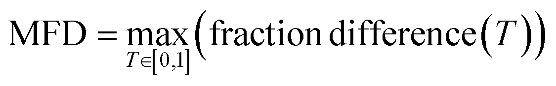
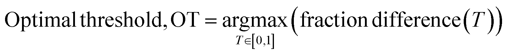
To quantitively assess the discriminative performance of different models after being trained, we propose the use of the maximum fraction difference (MFD). The fraction of ground-truth (orange) and query (blue) datasets that would be classified as positive can be calculated by setting the threshold to a specific normalised score for each model (eqn (1)). The fraction difference (eqn (2)) between these two datasets, as depicted by the red curve in Fig. 2(b), quantifies the discriminative capability under particular thresholds. The MFD corresponds to the maximum value (eqn (3)) of this curve, with superior models demonstrating higher MFD values. As shown in Fig. 2(b), the plot depicts fractions of both datasets for the poor model (left) and the successful model (right) as a function of the normalised score threshold, T, ranging from 0 to 1. The inherent characteristics of ML models, including their capacity to generalise and adapt to noise in the training data, means that not all ground-truth data will be given a normalised score close to 1. In such a case it is likely that ground-truth samples with normalised scores in the low score tail of the distribution represent a region of normalised score in which the model is not reliable in predicting true positive datapoints. For example, this may be due to entries in the ground-truth set which are in some way sufficiently dissimilar to other entries that a statistical model is unable to recognise that this entry should be labelled correctly. To discriminate between entries which are likely to be reliably predicted to be true positives and those which are not, we define the optimal threshold (OT) as the normalised score at which the MFD is achieved (eqn (4)). This threshold delineates the boundary between the reliable and unreliable regions for the predictive performance of the model, where entries in the query dataset with normalised scores above OT can reliably be predicted to have positive labels.

where the threshold, T, is chosen from the range of normalised scores [0,1].where the positive fraction is calculated for the fully ground-truth set and the query set respectively.

As stated above, the MFD is a metric designed to identify models where members of the query dataset with high scores have a high likelihood of being true positives. Such models may not have the highest true positive rate, representing a balance between maximising true positives while minimising false positives. In use cases where reducing the number of false negatives is most important, the TPR may be a better metric to consider.

The MFD is one method for comparing two distributions and can be compared to other established approaches for accomplishing the same task. A closely related metric is the two-sample Kolmogorov–Smirnov test⁴⁹ which uses the maximum absolute distance between the cumulative distribution functions of two distributions as a measure of their similarity. The MFD is better suited to the task of assessing the performance of OCC models since by retaining the sign of the difference OCC models that score the query dataset more highly than the ground truth dataset are penalised.

Models trained by different feature sets

To assess the performance of different descriptors in predicting MOF synthesisability, a total of 105 models are built and then compared implementing the MFD method, as illustrated in Fig. 3. For the systematic comparison of these models, 63 models were first trained employing seven OCC algorithms combined with nine distinct material representations formed by three sets of metal features and three distinct sets of linker features. As shown in Fig. 1, the metal feature sets are: (1) 6 elemental features that were identified important for MOF porosity prediction; (2) 6 elemental features along with 21-dimensional elemental features from magpie; (3) 6 elemental features along with 199-dimensional NLP-based features from mat2vec. The extended descriptor lists are shown in Table S2,† while the complete descriptor vector is available on the associated GitHub repository. The linker feature sets are: (1) 1613-dimensional linker features from Mordred; (2) 194-dimensional linker features from RDkit; (3) 2048-dimensional linker features from ECFPs with radius = 2. The normalised score distributions and positive fraction trends of the ground-truth and query datasets for these models are presented in Fig. S1–S9.† The optimal thresholds (OT) and the corresponding MFD values along with Kolmogorov–Smirnov test scores are listed in Table S3.†

Fig. 3 MFD values on seven approaches trained with three sets of metal features and five sets of linker features. Models are initially trained with the original 1613-dimensional Mordred features, 194-dimensional RDkit features, and the commonly employed 2048-dimensional ECFPs features (the full score distributions and positive fraction distributions are presented in Fig. S1–S9†). To address feature imbalance, additional training was performed using 177-dimensional Mordred features and 256-dimensional ECFPs features (the full score distributions and positive fraction distributions are presented in Fig. S10–S15†).

The dimensionality of the original 1613-dimensional Mordred features and the commonly employed 2048-dimensional ECFPs features markedly exceeds that of the metal features. Such discrepancy in dimensionality has the potential to adversely affect model performance due to an inherent imbalance in component representation. To balance the contribution on predictive results among the components, additional 42 models are generated based on linker representations with reduced dimensionality. Firstly, a pre-processing step to reduce the dimensionality of Mordred linker features is adopted by removing descriptors that are highly correlated with each other (describe similar properties), and those exhibit minimal changes across different instances (do not differentiate between instances).^32,50 This process specifically drops linker feature columns with Pearson correlation greater than 0.80 and low variance below 0.50, and retains 177 out of 1613 features. It is simultaneously useful to reduce the training time, save computational resources, and avoid overfitting and the “curse of dimensionality” while improving the overall performance of the models. The normalised score distributions for the 21 resulting models are shown in Fig. S10–S12.† The corresponding MFD and OT values are displayed in Fig. 3 and Table S4.† The length of the fingerprint for ECFPs is modifiable through the hyperparameter “bits”, which is associated with the final hash process that converts the chemical information into a fixed-length binary vector. In pursuit of balanced chemical component representations, models are trained using ECFPs linker features generated with 256 bits (refer to Fig. S13–S15 and Table S5†), generating a further 21 models.

Comparing the models trained using different metal features, most of those employing fewer features exhibit inferior performance in distinguishing between ground-truth and query datasets, as indicated by relatively low MFD values. This discernible pattern is consistently observed in moving from the far-left column of Fig. 3 to the far-right, particularly in models trained with ECFPs. Hence, it is posited that training models with 205-dimensional metal feature vectors containing both elemental features and NLP features leads to improved performance.

In the comparison of models trained with different linker features, it becomes apparent that, notably for IForest and OCSVM, those incorporating Mordred molecular features exhibit suboptimal performance, especially when trained with the complete set of 1613-dimensional Mordred features. The reduction in dimensionality of Mordred features enhances the performance of traditional models, as expected, but reduces the MFD observed for the DeepSVDD model. The similar trend can also be observed for models trained with ECFPs. To display this trend clearly, seven models are constructed with an additional 1024 bit ECFPs (Fig. S16–S18†) and subsequently compared. The corresponding OT and MFD values are listed in Table S6.† A comparison of the MFD values of the models trained using three different dimensional ECFPs is shown in Fig. S19.† The improved performance of the DeepSVDD model with higher-dimensional input can be attributed to the feature compression and sample reconstruction benefits provided by the autoencoder. Overall, it is evident that a feature space which is more balanced between metal and linker features generally results in improved score distributions in traditional models, minimising the overlap between the all-positive ground-truth dataset and the query dataset that includes a substantial but unknown number of negative samples. Traditional models and the LUNAR model exhibit their optimal performance measured by MFD when utilising 205-dimensional metal features and shorter 256 bit ECFPs, resulting in MFD values of 0.50, 0.48, 0.36, 0.44, 0.47, and 0.56 for IForest, KNN, OCSVM, LOF, CBLOF, and LUNAR, respectively. However, the DeepSVDD model demonstrates improved performance with identical 205-dimensional metal features and longer 2048 bit ECFPs, achieving an MFD value of 0.57.

For ECFPs feature sets, increasing the radius parameter allows for larger substructure information to be included. To test the effect of this, we build and compare models trained with ECFPs with larger radii, as shown in Fig. S20–S22 and Table S7–S8.† In traditional models, increasing the radius parameter does not yield higher MFD values with improved distinctions between the distributions of ground-truth and query data. On the contrary, for the DeepSVDD model, increasing the radius from 2 to 3 proves beneficial for generating an improved distribution to differentiate the ground-truth and query data with a higher MFD of 0.59, however the value of the MFD then decreased to 0.56 for yet higher radii.

In summary, the optimal performance as judged by the MFD is achieved with 205-dimensional metal features and 256 bit ECFPs (radius = 2) for traditional models and the LUNAR model. For DeepSVDD models, superior performance is observed with identical 205-dimensional metal features and 2048 bit ECFPs (radius = 3). This discrepancy arises from the requirement of balanced feature dimensions for classic models, whereas deep-learning models benefit from an excellent capacity to extract pertinent information from extensive datasets, thus showing a preference for higher-dimensional and more precise features. Regarding LUNAR, despite its neural network-based architecture, its learning capacity and performance are highly related to the conventional distance-based k-nearest neighbour computation process, resulting in a shared feature preference with traditional models. Fig. 4(a) lists the MFD value for models trained with these best-performing feature sets. To assess the stability and robustness of these models, 5-fold cross validation of MFD and OT values are implemented and shown in Fig. 4(c). Additionally, the sole available assessment metric, TPR, is calculated and displayed in Fig. S23.† MFD and TPR can be used as complementary assessment methods for the OCC problem, depending on the specific objectives. A higher TPR indicates a greater proportion of actual positives are correctly predicted as positive, whereas a higher MFD signifies a smaller proportion of actual negatives are wrongly predicted as positives. High TPR and high MFD signify better model performance. In cases like ours, where there is a need to reliably differentiate the ground-truth positive data from predominantly negative query data, a higher MFD is a more important indicator.

Fig. 4 (a) MFD values on seven OCC models trained with best-performing feature sets (205-dimensional metal features and 256 bits linker features from ECFPs (radius = 2) for IForest, KNN, OCSVM, LOF, CBLOF, and LUNAR; 205-dimensional metal features and 2048 bits linker features from ECFPs (radius = 3) for DeepSVDD); (b) seven OCC models trained with random features with identical feature dimensionality to (a). When training the LUNAR model with random features, the loss in the validation set (a percentage of training samples used for model validation, defined internally when using this model) consistently surpasses that in the training set, rendering the acquisition of valid results unattainable. (c) 5-fold cross validation of MFD and OT values. The black and blue lines represent respectively the mean value of MFD (the scale is given on the left) and OT (the scale is given on the right) in eight models, including the Euclidean distance model. The light grey and blue areas represent respectively the standard deviation of MFD and OT values in eight models. Models are trained with best-performing feature sets. MFD denotes maximum fraction difference, OT denotes optimal threshold.

To better illustrate the model's performance, we create a baseline model based on the Euclidean distance between each sample and its nearest neighbour in the training set, using 205-dimensional metal features and 256-dimensional ECFPs features, which are the same features used in our best-performing traditional models. As shown in the comparison in Fig. 4(c) and S23–S24,† the baseline outperforms the poorest-performing LOF, CBLOF, and OCSVM models with higher MFD and TPR. It exhibits relatively stable MFD with standard deviation notably smaller than that of IForest, CBLOF, and LUNAR, and a difference of less than 0.002 compared to other models. However, its TPR is less stable, with a standard deviation higher than all models except LUNAR. To demonstrate the utilisation of the domain knowledge by different models,⁵¹ we perform a comparative analysis using randomly generated features with identical dimensionalities to the best representations for each approach, as shown in Fig. 4(b) and S25.† Statistically significantly lower MFD values across all models trained with random features show that the domain knowledge captured in the 205 metal features and ECFPs is useful in making predictions. Although the MFD and Kolmogorov–Smirnov scores coincide for most models due to the shapes of their score distributions, the LUNAR model trained with random features in this case revealed a region with a negative “fraction difference”. As shown in Fig. S26,† the absolute value of the negative peak in the fraction difference curve is larger than that of its highest positive peak. Consequently, the Kolmogorov–Smirnov score is determined by the maximum absolute value of 0.38 in the region where fraction difference is negative, while the MFD value is based on the highest positive value of 0.17. This highlights the ability of the MFD method with a signed difference to correctly assess the very poor performance of models where scores in the query dataset are predicted to be higher than those in the ground-truth dataset.

Among all seven models, the DeepSVDD model stands out with the highest level of performance, as evidenced by its highest MFD value and relatively low spread across different cross-validation models (Fig. 4). LUNAR also shows a higher level of ability than other traditional models to distinguish the negative from positive, however, it exhibits inherent stochasticity, posing challenges in achieving stable predictions.

To further investigate the performance of the DeepSVDD model which obtained the highest MFD value of 0.59 on unseen data, we employ two additional approaches. In Fig. 5, a comparative analysis is presented, contrasting the performance of the DeepSVDD model with that of a poor IForest model trained with 6 elemental metal features and 1613-dimensional linker features from Mordred, with an MFD value of 0.08. In the first approach, we randomly remove 20% of the ground-truth data to create a positive validation dataset and use the remaining 80% of the data to train the models. The score distributions for the positive validation dataset are shown in green in Fig. 5(a). In the case of the IForest model, it perfectly overlaps with the distribution of the “all-positive” training dataset, exhibiting positive rates of 0.42 and 0.43, respectively. However, a substantial overlap is also observed with the query dataset which must include negative samples of [metal, linker] combinations that cannot synthesise MOFs, displaying a positive rate of 0.36. This is attributed to the limited ability of the model to differentiate between negative and positive instances, as indicated by the low MFD value. Conversely, the best-performing model demonstrates positive rates of 0.85, 0.61, and 0.24 for the training, validation, and query datasets respectively – the positive validation distribution in green follows the training distribution in orange but is distinctly different from the query dataset distribution shown in blue. These results affirm both the model's ability to correctly predict true positives, and its capability to distinguish between the negatives and positives in the query dataset. In the second approach, we use 14 true negative samples of metal and linker combinations which despite considerable effort experimentally were determined not to form a 3D MOF (see Methods section). The resulting predictions are shown in Fig. 5(b) and Table S9.† The DeepSVDD model correctly predicted that 12 of these [metal, linker] combinations would not form MOFs, compared to 8 for the IForest model, adding to our confidence that the predictions of the DeepSVDD model are better at discriminating between synthesisable and non-synthesisable MOFs.

Fig. 5 A comparison between a poor model on the left (IForest trained with 6 elemental metal features and 1613-dimensional linker features from Mordred, with an MFD value of 0.08) and the best-performing model on the right (DeepSVDD trained with 205-dimensional metal features and 2048-dimensional linker features from ECFPs, with an MFD value of 0.59). (a) Score distributions for the positive validation (green) dataset compared with the training data (main figure) and query dataset (the inset); (b) score distributions for the ground-truth (orange) and the query (blue) dataset, along with predictions for 14 true negative samples. Blue dots denote predictions as negative, while yellow dots denote predictions as positive. (c) Positive fraction distributions for the ground-truth (orange) and the query (blue) dataset, and the fraction difference (red) between these two datasets, versus normalised scores (ranging from 0 to 1). The vertical black dashed line in (b) and (c) indicates the OT (optimal threshold) value.

Having trained a model to predict MOF synthesisability from a given metal and linker combination, we combine its predictions with the porosity predictions for the query dataset generated using the random forest sequential models.³³ The synthesisability predictions using the best-performing DeepSVDD model and the predicted pore limiting diameters (PLDs) range for those combinations predicted to be synthesisable are shown in Fig. 6. By combining the synthesisability predictions and the porosity predictions, a list of combinations predicted to possess both high synthesisability and high guest accessibility is obtained. Consequently, the predictions revealed that 160 582 query combinations include a subset of 21 497 “large pores” pairs (i.e., PLD > 5.9 Å), a subset of 16 121 “medium pores” pairs (i.e., 4.4 Å < PLD < 5.9 Å), a subset of 31 194 “small pores” pairs (i.e., 2.4 Å < PLD < 4.4 Å), and a subset of 91 770 “non-porous” pairs (i.e., PLD < 2.4 Å). Among the 21 497 combinations categorised as exhibiting high PLD, 3453 also obtained high scores in the best DeepSVDD model, indicating their high probability of successful synthesis. We compile a list (Table S10†) comprising the top ten candidates derived from the best model, emphasizing their high synthesisability, catering to various pore size categories, spanning large, medium, and small.

Fig. 6 UMAP projection of the query dataset originating from 56-dimensional feature space used in porosity prediction model³³ coloured by (a) DeepSVDD predictions of MOF synthesisability and (b) porosity predictions of the PLD (pore limiting diameter) range. In panel (b), grey dots show datapoints with scores below OT (the optimal threshold, equals to 0.92 in the DeepSVDD model), while coloured dots indicate datapoints with synthesisability prediction scores above OT. Pink dots represent datapoints predicted to be non-porous (i.e. PLD < 2.4 Å), yellow dots represent datapoints predicted to have small pores (i.e. 2.4 Å < PLD < 4.4 Å), green dots represent datapoints predicted to have medium pores (i.e. 4.4 Å < PLD < 5.9 Å), and blue dots represent datapoints predicted to have large pores (i.e. PLD > 5.9 Å). Rectangular outlines with labels I, II, and III indicate clusters I, II, and III.

Separate clusters observed in Fig. 6 are formed by similar MOF-forming chemistries. Each cluster typically corresponds to a specific metal or a group of closely related metals paired with a set of linker molecules. However, there are also examples of clusters formed by one or several similar linkers and a list of metals. Observing the data distribution, synthetic and pore size predictions depicted in Fig. 6 enables us to identify potential chemical trends embedded in the results. Two small clusters (clusters I, II, as shown in Fig. 6(b)) can be observed where [metal, linker] combinations with scores above OT (the optimal threshold, equals to 0.92 in the DeepSVDD model) are all predicted to be non-porous, and a detailed analysis reveals that they are all combinations of [Ba] and various linkers (details are shown in ESI Part 2). Cluster I contains combinations of [Ba] with 146 distinct linkers predicted to be synthesisable, all linkers contain at least one five- or six-membered aromatic ring. In cluster II, the combination of [Ba] with 134 distinct linkers are predicted synthesisable, with the majority of linkers being aliphatic compounds. Another cluster (cluster III) comprises 100 combinations with 52 distinct metals and only two linkers, where all the predicted synthesisable combinations are predicted to have high porosity. There are other small clusters where combinations predicted to be synthesisable also provide consistent porosity predictions. Detailed information of all clusters is listed in ESI Part 2.

Conclusion

The utilisation of ML techniques has produced a surge of novel tools for materials discovery in recent years. However, various challenges emerge depending on the specific objectives. In the context of material synthesis, the primary challenge relates to the limited availability of the negative information for model learning and validation, highlighting the importance of better reporting of these data to enable more powerful predictive models in the future. This study presents an ML tool designed to help researchers identify the most promising synthesisable [metal, linker] combinations at the initial stages of novel MOF material design. Due to the limited availability of the vast majority of unreported “dark” (failed) reactions, OCC approaches are used to capture the underlying relationships between composition and synthesisability. To overcome the typical challenge arising from the absence of negative data in OCC problem, where classic evaluation metrics lose their validity, we propose a quantitative approach, the MFD method, as a complementary way to evaluate model performance and determine optimal thresholds for effective distinction between positives and negatives in a query dataset.

The MFD value provides a quantitative representation of the model's capacity to differentiate between the ground-truth dataset comprising solely of positive samples and the query dataset containing a significant proportion of true negatives. A higher value of the MFD indicates an enhanced ability of the model to identify instances dissimilar to the known positive ground-truth pattern. Following the extensive evaluation and comparison of trained models constructed using various feature representations and algorithms by implementing the MFD approach, we highlight the importance of a pre-processing step to keep the number of features of each component at the same order of magnitude when training models lacking feature compression capabilities. Conversely, for deep learning-based models capable of learning feature importance, the performance does not improve by applying the feature compression pre-processing step but rather by providing more relevant feature information. A deep learning-based model with best predictive capability as indicated by the highest MFD of 0.59 among all models is proposed: the DeepSVDD model. Given any combination of metal and linker, the model predicts the likelihood of them producing a 3D MOF material.

By combining this prediction with the porosity prediction, we generated a list of previously unexplored [metal, linker] combinations with high synthesisability and various pore sizes, offering a reference for material design. The significance of the models developed here lies in reducing the reliance on trial-and-error synthesis methods, providing valuable insights and guidance for researchers, and helping chemists prioritise the available options from the earliest material design stage.

Data availability

The data that support the findings of this study are openly available in https://github.com/zhangchi2025/MOF_synthesisability_prediction. The 1M1L3D dataset used to as the ground-truth dataset after removing duplicates is obtained from Pétuya et al. [DOI: https://doi.org/10.1002/anie.202114573]. This dataset is sourced from decomposing reported experimental three-dimensional MOF structures made of a single metal and a single linker in CSD (Data Update 3-2019) into their constituent components, and openly available in http://datacat.liverpool.ac.uk/1494.

Author contributions

Chi Zhang: methodology, software, visualization, investigation, formal analysis, writing – original draft. Dmytro Antypov: conceptualization, data curation, writing – review & editing, project administration. Matthew S. Dyer: conceptualization, supervision, writing – review & editing. Matthew J. Rosseinsky: conceptualization, supervision, writing – review & editing.

Conflicts of interest

The authors declare no conflict of interest.

Acknowledgements

This work is supported by China Scholarship Council (File No. 202104910051) and University of Liverpool. We thank Seth Wiggins, Aurelia Li and David Fairen-Jimenez for providing their list of 3D MOF. We thank Alexandros P. Katsoulidis and Elliot J. Carrington for providing the details of negative samples. We thank Leverhulme Trust for funding via the Leverhulme Research Centre for Functional Materials Design (RC-2015-036) and the UK Engineering and Physical Sciences Research Council (EPSRC) for funding through grant number EP/W036673/1.

References

1. Z. Wang, X. Huang, Y. Song and J. Xiao, 2017 IEEE 2nd International Conference on Big Data Analysis (ICBDA), 2017, pp. 478–482.
2. N. Seliya, A. Abdollah Zadeh and T. M. Khoshgoftaar, J. Big Data, 2021, 8, 122.
3. O. M. Yaghi, G. Li and H. Li, Nature, 1995, 378, 703–706.
4. A. G. Slater and A. I. Cooper, Science, 2015, 348, aaa8075.
5. O. M. Yaghi, J. Am. Chem. Soc., 2016, 138, 15507–15509.
6. I. G. Clayson, D. Hewitt, M. Hutereau, T. Pope and B. Slater, Adv. Mater., 2020, 32, 2002780.
7. S. Horike, S. Shimomura and S. Kitagawa, Nat. Chem., 2009, 1, 695–704.
8. H. Deng, C. J. Doonan, H. Furukawa, R. B. Ferreira, J. Towne, C. B. Knobler, B. Wang and O. M. Yaghi, Science, 2010, 327, 846–850.
9. J. R. Li, R. J. Kuppler and H. C. Zhou, Chem. Soc. Rev., 2009, 38, 1477–1504.
10. M. J. Kalmutzki, N. Hanikel and O. M. Yaghi, Sci. Adv., 2018, 4, eaat9180.
11. H. Furukawa, K. E. Cordova, M. O'Keeffe and O. M. Yaghi, Science, 2013, 341, 1230444.
12. W. Lu, Z. Wei, Z. Y. Gu, T. F. Liu, J. Park, J. Park, J. Tian, M. Zhang, Q. Zhang, T. Gentle III, M. Bosch and H. C. Zhou, Chem. Soc. Rev., 2014, 43, 5561–5593.
13. O. M. Yaghi, M. O'Keeffe, N. W. Ockwig, H. K. Chae, M. Eddaoudi and J. Kim, Nature, 2003, 423, 705–714.
14. P. G. Boyd, A. Chidambaram, E. Garcia-Diez, C. P. Ireland, T. D. Daff, R. Bounds, A. Gladysiak, P. Schouwink, S. M. Moosavi, M. M. Maroto-Valer, J. A. Reimer, J. A. R. Navarro, T. K. Woo, S. Garcia, K. C. Stylianou and B. Smit, Nature, 2019, 576, 253–256.
15. Y. Pramudya, S. Bonakala, D. Antypov, P. M. Bhatt, A. Shkurenko, M. Eddaoudi, M. J. Rosseinsky and M. S. Dyer, Phys. Chem. Chem. Phys., 2020, 22, 23073–23082.
16. A. M. Tollitt, R. Vismara, L. M. Daniels, D. Antypov, M. W. Gaultois, A. P. Katsoulidis and M. J. Rosseinsky, Angew. Chem., Int. Ed., 2021, 60, 26939–26946.
17. H. Demir, H. Daglar, H. C. Gulbalkan, G. O. Aksu and S. Keskin, Coord. Chem. Rev., 2023, 484, 215112.
18. K. T. Butler, D. W. Davies, H. Cartwright, O. Isayev and A. Walsh, Nature, 2018, 559, 547–555.
19. K. M. Jablonka, D. Ongari, S. M. Moosavi and B. Smit, Chem. Rev., 2020, 120, 8066–8129.
20. A. Nandy, C. Duan and H. J. Kulik, J. Am. Chem. Soc., 2021, 143, 17535–17547.
21. C. M. Collins, L. M. Daniels, Q. Gibson, M. W. Gaultois, M. Moran, R. Feetham, M. J. Pitcher, M. S. Dyer, C. Delacotte, M. Zanella, C. A. Murray, G. Glodan, O. Perez, D. Pelloquin, T. D. Manning, J. Alaria, G. R. Darling, J. B. Claridge and M. J. Rosseinsky, Angew. Chem., Int. Ed., 2021, 60, 16457–16465.
22. G. Han, A. Vasylenko, L. M. Daniels, C. M. Collins, L. Corti, R. Chen, H. Niu, T. D. Manning, D. Antypov, M. S. Dyer, J. Lim, M. Zanella, M. Sonni, M. Bahri, H. Jo, Y. Dang, C. M. Robertson, F. Blanc, L. J. Hardwick, N. D. Browning, J. B. Claridge and M. J. Rosseinsky, Science, 2024, 383, 739–745.
23. A. Vasylenko, J. Gamon, B. B. Duff, V. V. Gusev, L. M. Daniels, M. Zanella, J. F. Shin, P. M. Sharp, A. Morscher, R. Chen, A. R. Neale, L. J. Hardwick, J. B. Claridge, F. Blanc, M. W. Gaultois, M. S. Dyer and M. J. Rosseinsky, Nat. Commun., 2021, 12, 5561.
24. P. Z. Moghadam, A. Li, S. B. Wiggin, A. Tao, A. G. P. Maloney, P. A. Wood, S. C. Ward and D. Fairen-Jimenez, Chem. Mater., 2017, 29, 2618–2625.
25. P. G. Boyd, Y. Lee and B. Smit, Nat. Rev. Mater., 2017, 2, 17037.
26. C. Mellot-Draznieks, J. Dutour and G. Ferey, Angew. Chem., Int. Ed., 2004, 43, 6290–6296.
27. B. A. Helfrecht, G. Pireddu, R. Semino, S. M. Auerbach and M. Ceriotti, Digital Discovery, 2022, 1, 779–789.
28. D. Gleaves, N. Fu, E. M. Dilanga Siriwardane, Y. Zhao and J. Hu, Digital Discovery, 2023, 2, 377–391.
29. N. C. Frey, J. Wang, G. I. Vega Bellido, B. Anasori, Y. Gogotsi and V. B. Shenoy, ACS Nano, 2019, 13, 3031–3041.
30. E. R. Antoniuk, G. Cheon, G. Wang, D. Bernstein, W. Cai and E. J. Reed, NPJ Comput. Mater., 2023, 9, 155.
31. J. Jang, J. Noh, L. Zhou, G. H. Gu, J. M. Gregoire and Y. Jung, Matter, 2024, 7, 2294–2312.
32. A. Vriza, A. B. Canaj, R. Vismara, L. J. Kershaw Cook, T. D. Manning, M. W. Gaultois, P. A. Wood, V. Kurlin, N. Berry, M. S. Dyer and M. J. Rosseinsky, Chem. Sci., 2021, 12, 1702–1719.
33. R. Petuya, S. Durdy, D. Antypov, M. W. Gaultois, N. G. Berry, G. R. Darling, A. P. Katsoulidis, M. S. Dyer and M. J. Rosseinsky, Angew. Chem., Int. Ed., 2022, 61, e202114573.
34. R. Banerjee, A. Phan, B. Wang, C. Knobler, H. Furukawa, M. O'Keeffe and O. M. Yaghi, Science, 2008, 319, 939–943.
35. L. Ward, A. Agrawal, A. Choudhary and C. Wolverton, NPJ Comput. Mater., 2016, 2, 16028.
36. V. Tshitoyan, J. Dagdelen, L. Weston, A. Dunn, Z. Rong, O. Kononova, K. A. Persson, G. Ceder and A. Jain, Nature, 2019, 571, 95–98.
37. R. J. Murdock, S. K. Kauwe, A. Y.-T. Wang and T. D. Sparks, Integr. Mater. Manuf. Innovation, 2020, 9, 221–227.
38. H. Moriwaki, Y. S. Tian, N. Kawashita and T. Takagi, J. Cheminform., 2018, 10, 4.
39. RDKit: Open-source cheminformatics, https://www.rdkit.org.
40. H. L. Morgan, J. Chem. Doc., 1965, 5, 107–113.
41. D. Rogers and M. Hahn, J. Chem. Inf. Model., 2010, 50, 742–754.
42. M. M. Breunig, H. P. Kriegel, R. T. Ng and J. Sander, ACM Sigmod Record, 2000, 29, 93–104.
43. A. Goodge, B. Hooi, S. K. Ng and W. S. Ng, Proc. AAAI Conf. Artif. Intell., 2022, 36, 6737–6745.
44. L. Ruff, R. A. Vandermeulen, N. Görnitz, L. Deecke, S. A. Siddiqui, A. Binder, E. Müller and M. Kloft, Proceedings of the 35th International Conference on Machine Learning, PMLR 80, 2018, pp. 4393–4402.
45. Z. Yue, N. Zain and L. Zheng, J. Mach. Learn. Res., 2019, 20, 1–7.
46. J. Lee, Y. Lee, J. Kim, A. R. Kosiorek, S. Choi and Y. W. Teh, Proceedings of the 36th International Conference on Machine Learning, PMLR 97, 2019, pp. 3744–3753.
47. J. Bergstra, B. Komer, C. Eliasmith, D. Yamins and D. D. Cox, Comput. Sci. Discov., 2015, 8, 014008.
48. J. Bekker and J. Davis, Mach. Learn., 2020, 109, 719–760.
49. Y. Dodge, in The Concise Encyclopedia of Statistics, Springer New York, New York, NY, 2008, pp. 283–287,  DOI:10.1007/978-0-387-32833-1_214.
50. S. Velliangiri, S. Alagumuthukrishnan and S. I. Thankumar joseph, Procedia Comput. Sci., 2019, 165, 104–111.
51. S. Durdy, M. W. Gaultois, V. V. Gusev, D. Bollegala and M. J. Rosseinsky, Digital Discovery, 2022, 1, 763–778.

---

Footnote

† Electronic supplementary information (ESI) available. See DOI: https://doi.org/10.1039/d4dd00161c

---