Automated processing of chromatograms: a comprehensive python package with a GUI for intelligent peak identification and deconvolution in chemical reaction analysis

Abstract

Reaction screening and high-throughput experimentation (HTE) coupled with liquid chromatography (HPLC and UHPLC) are becoming more important than ever in synthetic chemistry. With a growing number of experiments, it is increasingly difficult to ensure correct peak identification and integration, especially due to unknown side components which often overlap with the peaks of interest. We developed an improved version of the MOCCA Python package with a web-based graphical user interface (GUI) for automated processing of chromatograms, including baseline correction, intelligent peak picking, peak purity checks, deconvolution of overlapping peaks, and compound tracking. The individual automatic processing steps have been improved compared to the previous version of MOCCA to make the software more dependable and versatile. The algorithm accuracy was benchmarked using three datasets and compared to the previous MOCCA implementation and published results. The processing is fully automated with the possibility to include calibration and internal standards. The software supports chromatograms with photo-diode array detector (DAD) data from most commercial HPLC systems, and the Python package and GUI implementation are open-source to allow addition of new features and further development.

---

Introduction

Synthetic organic chemistry is currently witnessing a significant paradigm shift, powered by advancements in automation and digital chemistry. At the same time, the chemical industry faces increasing pressure on timelines and costs in the discovery and development of innovative molecules and their corresponding chemical processes.^1,2 In the face of these challenging circumstances, automation and digital chemistry are both directly contributing to reducing the costs and accelerating the timelines by increasing the experimental throughput (reaction execution, reaction analytics, design & decision-making) and reducing the number of synthetic experiments required thanks to modelling and predictive models.^3–6 Initially, academia and industry largely focused on the development and adoption of fully automated platforms for reaction execution, such as high-throughput experimentation (HTE).^7,8 With the advent of data-science driven reaction designs and decision-making processes, the two areas of automation and digital chemistry are becoming increasingly intertwined.⁹ Until recently, reaction analytics has not received much attention by the community, despite its pivotal role as the interface between chemical experiments and data-driven design & decision-making. Importantly, the quality of this interface determines the efficiency and reliability when generating data.^10,11 This fact becomes especially evident when going from human-in-the-loop to closed-loop workflows, wherein experiments are autonomously performed. Reliable and high-quality reaction analysis data are required to maintain the self-driving platform operative without human interventions.^12–14

The most commonly used analytical methods for HTE and chemical reaction analysis in general are high-performance liquid chromatography (HPLC) and ultra-high-performance liquid chromatography (UHPLC).⁷ Commercial solutions for automated liquid chromatography analysis exist,^15–19 but remain locked in vendor-specific proprietary software and therefore pose a challenge for user-specific integration into established workflows.^20,21 When dealing with hundreds or thousands of chromatograms, it is difficult to ensure that all peaks are automatically integrated correctly, especially in the presence of unexpected side components which might overlap with the product or substrate peaks. Although automatic chromatogram processing has been the focus of many publications, most programs do not take advantage of the multidimensionality of the HPLC-DAD (photo-diode array detector) raw data and therefore fail to handle and deconvolute overlapping peaks.^11,22–24 This can lead to labor-intensive, manual inspection and analysis of the HPLC data, which must be avoided, especially in the context of automated laboratories. Therefore, multivariate deconvolution should be used to reliably predict the number of peak components and deconvolute the components correctly.²⁵

As part of our effort to make automated chromatogram processing more reliable and accessible, we have recently introduced MOCCA (Multivariate Online Contextual Chromatographic Analysis) for chemical reaction analysis of HPLC-DAD raw data and demonstrated its broad applicability to both automated and non-automated use cases.¹⁰ By releasing MOCCA as an open-source Python package, we aim to create a community project that overcomes the limitations of vendor software and enables easy implementation into automated workflows according to the user needs. In this spirit, we have continued working on the MOCCA tool and developed an improved Python package for automated processing of chromatograms, including baseline correction, intelligent peak picking, peak purity checks, deconvolution of overlapping peaks, and compound tracking. The processing is fully automated with the possibility to include calibration and internal standards. The individual automatic processing steps have been improved to make the software more dependable and versatile. The algorithm accuracy was benchmarked on three datasets and compared to previous MOCCA implementation and published results. We have developed a new, web-based graphical user interface (GUI) to make the software accessible to users with limited programming experience and to facilitate routine use in a laboratory environment. The software supports chromatograms with photo-diode array detector (DAD) data from most commercial HPLC systems, and the Python package and GUI implementation are open-source to allow addition of new features and further development.

This paper aims to provide a detailed overview of the improved chromatographic processing steps, the newly developed GUI and the application of MOCCA for chemical reaction analysis.

Methods

Chromatogram processing

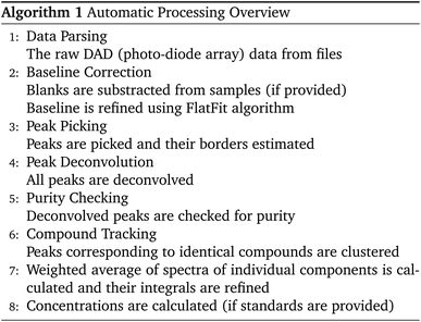
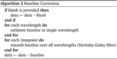
The Python package and GUI support fully automated processing of sets of chromatograms; the general outline is shown in algorithm 1 and details are described in the following section:

Data parsing. The MOCCA package supports files from most common commercial software, including Empower from Waters, ChemStation from Agilent, and LabSolutions from Shimadzu. Parsers for additional formats can be added easily.²⁶

Baseline correction. A good baseline is crucial for peak picking, integration, deconvolution, and purity checking; thus, it is important to have a reliable baseline correction algorithm. MOCCA's implementation of baseline correction of the DAD data follows algorithm 2.

In practice it is recommended to subtract the blank from sample data before estimating the baseline. The baseline z(t) of 1D data y(t) is estimated by minimizing the loss function as defined using different algorithms AsLS,^27–29 arPLS,²⁹ or FlatFit (Table 1), which are described in more detail below.

Table 1 Comparison of loss functions for baseline estimation algorithms. For AsLS, the asymmetry factor p is usually in the range of 10⁻⁵ to 0.01.²⁷ For arPLS, the parameter α determines how sensitive the baseline is to negative noise or peaks; this is somewhat analogous to p in AsLS. For FlatFit, the weighting function is based on normalized first and second derivatives of the data; ε prevents division by zero

AsLS	arPLS	FlatFit
	d(t) = y(t) − z(t)
	m = mean of d(t), where d(t) < 0
	s = std dev. of d(t), where d(t) < 0	ε = 10^−7

---

The derivatives are calculated using finite differences or the Savitzky–Golay filter, and the integrals are calculated numerically by summing the data points.

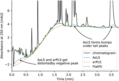
Asymmetric least squares (AsLS)²⁷. Asymmetric least squares regression with smoothness penalty is a simple and popular algorithm for baseline estimation. The loss function (Table 1) has two terms: an asymmetrically weighted squared difference between baseline and data and smoothness penalty which can be tuned using λ. The drawbacks of AsLS are that the baseline has a tendency to form positive bumps under tall peaks, and it is highly distorted if any negative peaks are present (Fig. 1).

Fig. 1 Comparison of baseline estimation using AsLS, arPLS and FlatFit algorithms on a representative chromatogram of a reaction mixture measured at 250 nm without blank subtraction. Typically, the baseline would be first corrected by subtracting a blank chromatogram and only then refined using a baseline estimation algorithm. The blank was not subtracted in this case to highlight the differences between the different algorithms.

Asymmetrically reweighted penalized least squares (arPLS)²⁹. The arPLS method improves on the AsLS method by making the weighting function w(t) sigmoidal (Table 1), removing bumps under tall peaks. However, the arPLS method relies on a small amount of background noise being present, and it can also be highly distorted by negative peaks (Fig. 1).
Flatness weighted fit (FlatFit). The newly developed FlatFit algorithm takes a different approach to AsLS and arPLS. Instead of basing the weighting function w(t) on the difference between the baseline and signal, it uses normalized first and second derivatives to predict which parts of the spectrum are peaks and which are baselines (Table 1).

Unlike AsLS and arPLS which are minimized iteratively, FlatFit has a single closed-form solution. Additional advantages are that the baseline can be estimated for signals with both positive and negative peaks, and there are no additional parameters which need to be tuned.

For typical chromatogram data, FlatFit and arPLS perform similarly well, outperforming AsLS. Both FlatFit and arPLS have their respective weaknesses – FlatFit overestimates the baseline in areas with many peaks, while arPLS cannot handle negative peaks. By default, we use FlatFit to avoid convergence problems and parameter tuning.

Peak picking. For successful deconvolution and peak integration, it is important to find all significant peaks and correctly determine their borders. The peak picking procedure follows algorithm 3 and the individual steps are visualized in Fig. 2.

Fig. 2 Visualized peak picking procedure on a representative chromatogram of a reaction mixture. From top: first, maxima are found and filtered, background noise is estimated, and peak borders are expanded to contain the entire peak. Secondly, overlapping borders are merged. Lastly, peaks that have sufficient separation between maxima are split. All resulting peaks are subsequently passed to the deconvolution algorithm to resolve overlapping peaks or confirm purity.

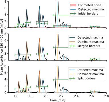
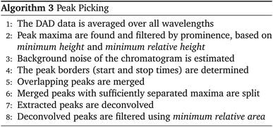
The entire peak picking procedure is carried out using 1D data which are obtained by averaging the DAD data over all wavelengths. Once the peak maxima are located and filtered, the peak borders are found using estimated background noise and the signal slope. The peaks are then further refined by merging overlapping peaks and splitting peaks with sufficient separation. After this procedure, the peaks are ready to be passed to the deconvolution algorithm.

The peak significance is determined using three conditions: minimum height, minimum relative height, and minimum relative area.†

To determine peak borders, background noise is estimated and the chromatogram is then scanned from the peak maximum until the absorbance is lower than background noise. This ensures that peaks are not cut off prematurely.

Peak deconvolution. Peak deconvolution is a process of explaining experimental chromatogram data D(t, λ) by predicting concentration profiles c_i(t) and absorption spectra s_i(λ) of pure components i ∈ {1,…,N} in order to minimize the sum of squares of the residual error ε(t, λ) (eqn (1)‡).

If c_i(t) and s_i(λ) are not constrained, the problem is under-determined.³⁰ Thus, we constrain the concentration profiles to a peak shape model, and the absorption spectra are strictly non-negative.^25,30 By default, the new MOCCA version uses the bidirectional exponentially modified Gaussian (BEMG) peak model,³⁰ but the package also implements other popular peak shape models including Fraser-Suzuki and BiGaussian.³¹

The parameters determining the peak shape and their naming conventions and interpretation vary between models. Furthermore, due to the mathematical nature of some of the models, parameters are often correlated with multiple peak properties (for example increasing tailing often slightly shifts the peak maximum to the right). Parameters and their main effects for selected models are:

• BiGaussian

– h: height of the peak

– μ: elution time (position of peak maximum)

– σ₁: width of the left half of the peak

– σ₂: width of the right half of the peak

• Fraser-Suzuki

– h: height of the peak

– μ: elution time (position of peak maximum)

– σ: width of the peak

– α: peak tailing

• BEMG

– h: height of the peak

– μ: elution time (position of peak maximum)

– σ: width of the peak

– a: peak tailing

– b: peak fronting

However, if accurate peak properties that are consistent between models, such as peak height, location of peak maximum or width at 50% height, are required, it is best to measure them from the calculated peak shape.

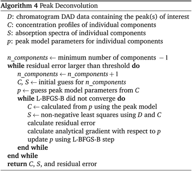
During peak deconvolution, the number of components is iteratively increased until the residual error is smaller than some user-specified threshold,§ similar to the approach published by Erny.²⁵ The deconvolution procedure (algorithm 4) is based on the L-BFGS-B optimizer (memory limited Broyden–Fletcher–Goldfarb–Shanno algorithm with bounds).

Parallel factor analysis (PARAFAC)³² and independent component analysis (ICA)³³. Parallel factor analysis (PARAFAC)³² and independent component analysis (ICA)³³ are alternative approaches for signal deconvolution that can be used to resolve overlapping peaks in chromatograms,³⁴ PARAFAC was used in the previous MOCCA version.¹⁰ Unlike our new approach which constrains peak shapes, ICA maximizes signal independence measured using neg-entropy, and PARAFAC constrains the concentration profiles and spectra to be the same across multiple chromatograms (eqn (2)¶). For ICA or PARAFAC to have a unique solution, the number of chromatograms needs to be equal to or larger than the number of compounds.
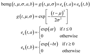
Bidirectional exponentially modified Gaussian (BEMG) model³⁰. Inspired by the exponentially modified Gaussian (EMG) peak shape model for liquid chromatography,³⁵ the BEMG model is defined as convolution of the Gaussian function and two decaying exponentials (eqn (3)||).

The BEMG function further extends the EMG model, allowing for peak fronting and symmetric distortions, as shown in Fig. 3. Overall, the BEMG function is very flexible and can describe a wide range of peak shapes.

Fig. 3 Examples of possible peak shapes using the BEMG model, including different widths, symmetric distortion, fronting, and tailing. (A) σ = 0.3, a = 100, b = 100, (B) σ = 0.2, a = 100, b = 100, (C) σ = 0.05, a = 5, b = 5, (D) σ = 0.1, a = 3, b = 100, and (E) σ = 0.1, a = 100, b = 3. All peaks are normalized to have equal height.

Purity checking. It is good practice to check all integrated peaks for purity. Unlike with manual analysis or most vendor software, where peak purity is either not checked at all or checked only for selected peaks, MOCCA automatically checks purity of all peaks in all chromatograms, and all impure peaks are deconvoluted to recover the separate components.

The accuracy of purity checking and deconvolution strongly depends on how similar the retention times and absorbance spectra of the overlapping peaks are.**

For a peak to be considered pure, or successfully deconvoluted, it must satisfy the following conditions.

• The number of components is equal to or higher than the number of significant maxima in the chromatogram (significant maxima are considered to be any maxima detected by the peak picking algorithm)

• The residual error after deconvolution is sufficiently small.††

Thus, even putatively pure peaks are deconvoluted using a single component to test for purity. The advantage of this approach is that purity checks are consistent for peaks with any number of components.

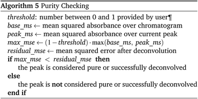
Whether the residual error after deconvolution is sufficiently small is checked by algorithm 5.

The algorithm 5 is analogous to setting the R² threshold. If the local threshold for a single peak is low, it will be increased to a global threshold shared across the entire chromatogram base_ms; this is useful to prevent over-deconvoluting small peaks which contain significant amounts of random noise.

Compound tracking. After deconvolution, peaks across all chromatograms are compared and identical compounds are clustered together. Two peaks are considered to correspond to identical compounds if their retention times are sufficiently close and the Pearson correlation of their spectra is higher than the user-specified threshold.‡‡

Retention times t₁ and t₂ are considered to be sufficiently close if |t₁ – t₂| < τ(w₁ + w₂)/2, where w_i are peak widths and τ is the user-specified threshold. Thanks to the adaptive threshold, τ does not need to be adjusted for peaks with varying widths.

Graphical user interface

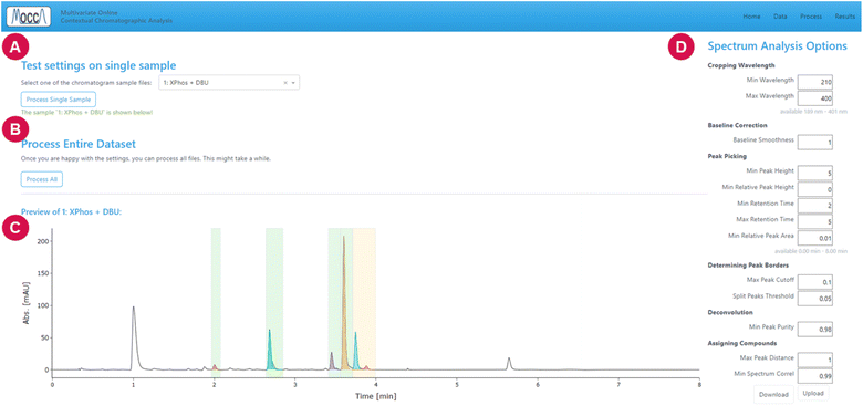
The GUI is often overlooked during scientific software development, despite its importance for accessibility and usability, especially for users without excessive programming experience. We designed the GUI for MOCCA to be simple and efficient and to give users direct control over their data, the processing pipeline, and the results. A user-friendly GUI is especially important in laboratory settings where speed and reliability are critical.

The GUI is a web application built in Dash, so that the data can be processed either on a local-host server, or in a more centralised manner. Together with the modular code base, this simplifies addition of new features and allows for many possible deployment options.

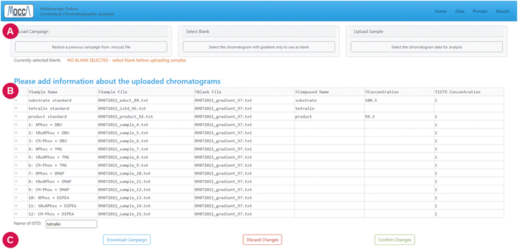
The current GUI guides the user through three major steps: uploading data, data processing, and interpretation of results.

GUI: data page. In the data page (Fig. 4), the user is prompted to upload the raw chromatogram data and blanks and specify names and concentrations of compound standards. The program can work without standards too, but if the information is provided, absolute concentrations and/or concentrations relative to internal standards are automatically calculated. This is much faster and less error-prone compared to doing the calculations manually in a spreadsheet.

Fig. 4 Data page. (A) Areas for uploading data; it is possible to restore previous data (campaign), or to upload blanks and samples. (B) This table displays information about samples, and the user can rename the samples or specify information about compound standards and internal standards. (C) Buttons for confirming changes, discarding changes, and for downloading the entire dataset (campaign) into a .mocca2 file (JSON compressed using GZIP).

GUI: processing page. After uploading all data, the user can adjust processing settings (Fig. 5). Although the default settings work on most samples, the GUI gives the flexibility to tune all the settings as needed.

Fig. 5 Processing page. (A) Directive to test settings by processing a single selected chromatogram. (B) Directive to process the entire dataset. (C) Processed and deconvoluted chromatogram to check the settings. The individual deconvoluted compounds are plotted in different colors; background color indicates the deconvolution result; green – single pure compound; yellow – successfully deconvoluted overlapping compounds; red – deconvolution failed. (D) Processing settings, with an option to export and import settings. All settings are also explained lower on this page.

The settings can be tested by processing a single chromatogram, and it is possible to save or reload the settings using a .yaml file. When the user is satisfied with the settings, all chromatograms can be processed with a single click on the “process all” button.

GUI: results page. The results page serves two major purposes: it allows the user to efficiently check the correctness of the processed data and summarizes the results to make them easy to understand and export.

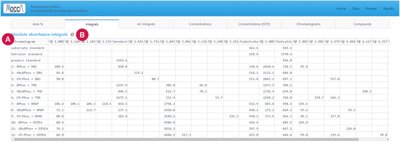
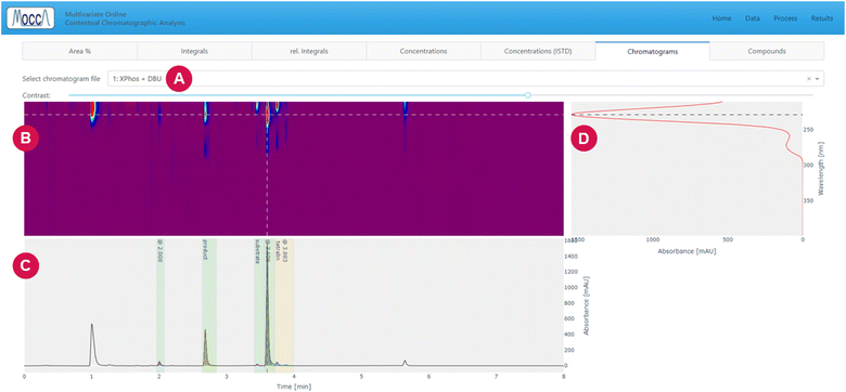
The page is divided into multiple tabs, which let the user view the peak integrals and calculated concentrations (tabs “area%”, “integrals”, “rel. integrals”, “concentrations”, and “rel. concentrations”, Fig. 6), inspect the deconvoluted chromatograms (tab “chromatograms”, Fig. 7), and see a summary of all compounds found across all chromatograms (tab “compounds”).

Fig. 6 Results page, “integrals” tab. (A) Table summarizing the integrals of individual compounds in all chromatograms. (B) This icon copies the raw data into the clipboard and lets the user paste the data into spreadsheet software or a .csv file.

Fig. 7 Results page, “chromatograms” tab. (A) Dropdown for selecting the chromatogram. (B) Heatmap of the DAD data, and the contrast can be adjusted using the slidebar above. (C) Chromatogram with deconvoluted peaks at a single wavelength; the wavelength can be changed by clicking the heatmap or absorbance plot. (D) Absorbance spectrum at a given time; the time can be changed by clicking the heatmap or chromatogram plot.

Despite the automatic processing, most chemists are still interested in checking the data visually. The GUI provides an option to interactively inspect the DAD data using a heatmap and cross-sections for specified time and wavelength, allowing to zoom into specific regions and adjust the heatmap contrast (Fig. 7).

Results

To highlight MOCCA's improved performance and broad applicability, we studied three different use cases and directly compared them to the previous MOCCA implementation and published results: (i) deconvolution of overlapping peaks with similar spectra; (ii) re-evaluation of reaction kinetics study on a Knoevenagel condensation reaction; (iii) benchmarking and peak deconvolution accuracy comparsion on a dataset with diterpene esters.

Deconvolution of diphenylphosphonic acid and diphenylphosphine oxide

Diphenyl phosphonic acid and diphenylphosphine oxide (Fig. 8) have nearly identical UV-vis spectra, which allows us to demonstrate the advantage of fitting peak shapes.

Fig. 8 Structures of diphenylphosphonic acid (1) and diphenylphosphine oxide (2).

The disadvantage of PARAFAC is that multiple chromatograms containing the same compounds are needed for deconvolution and that it assumes identical peak shapes for the same compound across multiple chromatograms. ICA also does not provide a satisfactory solution, as the concentrations and absorption spectra might be negative and the peak shapes are often nonphysical. Moreover, modelling peak shapes seems to be advantageous – the BEMG model is flexible enough to accommodate most possible shapes, it prevents overfitting artifacts, and it also allows to deconvolute compounds with nearly identical absorption spectra using their peak shapes (Fig. 9).

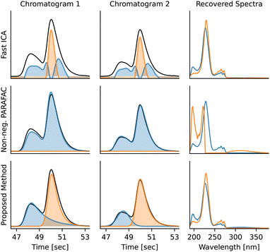Fig. 9 Deconvolution of overlapping peaks with similar spectra using Fast ICA,³⁶ non-negative PARAFAC, and multivariate peak fitting. Because of the nearly identical spectra, Fast ICA and PARAFAC fail completely to deconvolute the peaks. PARAFAC needs both chromatograms to deconvolute the compounds, while Fast ICA and the multivariate peak fitting implemented by MOCCA process the chromatograms independently. The overlapping peaks are diphenylphosphinic acid (1) and diphenylphosphine oxide (2) respectively.

Kinetics of Knoevenagel condensation

To compare the accuracy of the new algorithm to that of the original MOCCA version, we used the Knoevenagel condensation dataset (Fig. 10).¹⁰

Fig. 10 Kinetic data from Knoevenagel condensation between benzaldehydes 3a–c and malononitrile 4 was used to test deconvolution accuracy of MOCCA for peaks with varying integrals and overlaps.

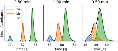
The dataset contains standards of benzaldehyde (3a), 4-methoxybenzaldehyde (3b) and 4-(dimethylamino)benzaldehyde (3c) and kinetic data from the condensation reactions. The samples have been run at different gradient lengths (0.5–2.5 min) to obtain different degrees of overlap between the peaks (Fig. 11).

Fig. 11 Different gradient lengths can be used to achieve different degrees of overlap between the peaks of benzaldehyde derivatives 3a, 3b and 3c. The dataset contains chromatograms with gradient lengths of 0.5, 0.75, 1.0, 1.5 and 2.5 minutes, and only selected gradient lengths are shown here.

The calibration chromatograms were used to compare the integration accuracy of pure peaks (Table 2) using (A) the previous version of MOCCA with PARAFAC, (B) the new MOCCA version with peaks constrained to the BEMG shape model, and (C) with subsequently relaxed concentration profiles.§§ The significant improvement of the new MOCCA version (Table 2, B and C compared to A) is caused mostly by more accurate baseline correction. It is also apparent that constraining peak shape decreases the integration accuracy for pure peaks (Table 2, B vs. C), although for overlapping peaks the opposite is often true.

Table 2 Comparison of integration accuracy of 3a, 3b and 3c standards. The entries represent R² values for linear fit of MOCCA integrals against manual integrals with the intercept fixed to 0. A: previous MOCCA version using PARAFAC, B: new MOCCA version with peak shape constrained to the BEMG model, and C: the absorption spectra were estimated using new MOCCA deconvolution with the BEMG peak model, and the concentration profiles were then recalculated using non-negative least squares, relaxing the peak shape constraint

Gradient length	A^10	B	C
2.50 min	0.9994	0.99987	0.999996
1.50 min	0.9993	0.99954	0.999997
1.00 min	0.9997	0.99987	0.999996
0.75 min	0.9995	0.99980	0.999997
0.50 min	0.9997	0.99989	0.999989

---

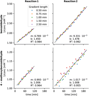
This set the stage to re-evaluate the chromatograms from kinetic experiments where the peaks of benzaldehyde derivatives overlap. For the kinetic plot of 3a, the obtained R² values (0.984 and 0.992) are significantly better compared to values using old MOCCA¹⁰ (0.965 and 0.960). We also managed to obtain kinetic plots for 3b, which were too noisy when using the old MOCCA version and thus were not reported previously (Fig. 12).¹⁰ Benzaldehyde derivative 3c essentially does not react throughout the measured reaction course.

Fig. 12 Pseudo-second order kinetic plots of 3a and 3b derived from competition experiments in the Knoevenagel condensation recorded with five different gradient length runs and analyzed with the new MOCCA version. Reaction 1 contains 3a and 3b and Reaction 2 contains 3a, 3b and 3c. The data are fitted with straight line y = mx + b.

Accuracy of deconvolution of diterpene esters

Further benchmarking was done on a published dataset with deterpene esters (Fig. 13),³⁷ and the accuracy of peak deconvolution was compared to that of a similar deconvolution method published by Erny.²⁵ The dataset consists of 16 chromatograms, each of which contains a mixture of kahweol oleate (KO, 6), kahweol palmitate (KP, 7), cafestol oleate (CO, 8) and cafestol palmitate (CP, 9) (Fig. 14) with known concentrations. Similar to Erny,²⁵ we deconvoluted the peaks, constructed linear calibration curves for the individual components (Fig. 14), and used the R² values to compare the integration accuracy (Table 3). The accuracy of the new MOCCA version using FlatFit baseline correction and the BEMG peak model is comparable to that obtained by Erny.²⁵ Using other models, such as arPLS for baseline correction or the Fraser-Suzuki peak model, decreases the integration accuracy. The peaks were deconvoluted without any standards of the pure components; this would have not been possible using the previous MOCCA version with PARAFAC.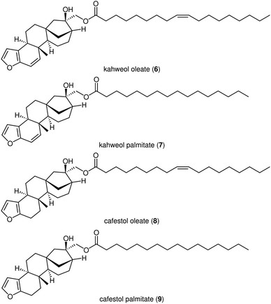

Fig. 13 Structures of diterpene esters in the dataset published by Erny.²⁵

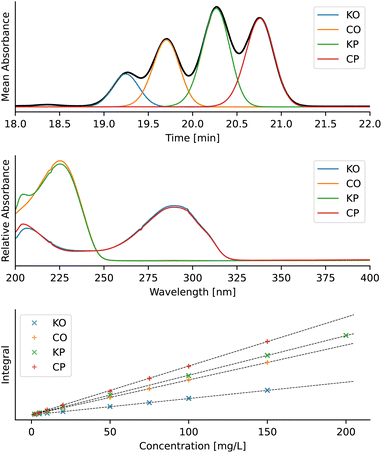Fig. 14 Deconvolution results of diterpene esters. From top: example of the deconvoluted chromatogram, recovered absorption spectra of individual diterpene esters, and linear calibration curves. The data in the figure are from calibration sample 16,³⁷ the baseline was corrected using FlatFit and the peaks were deconvoluted using the BEMG model. Chromatograms were analysed in the 18–22 minute interval over the entire provided UV-vis spectrum (200–400 nm).

Table 3 Integration accuracy of diterpene esters using different deconvolution methods. The entries represent R² values of linear calibration curves

Method	KO	CO	KP	CP
BEMG and FlatFit	0.99980	0.99991	0.99997	0.99976
BEMG and arPLS	0.99971	0.99983	0.99993	0.99975
Fraser-Suzuki and FlatFit	0.99807	0.99827	0.99971	0.99779
itMPF + fminsearch^25	0.99990	0.99991	0.99997	0.99980
itMPF + fminnunc^25	0.99979	0.99991	0.99996	0.99972

---

Conclusions

We present an improved MOCCA Python package with a newly developed web-based graphical user interface. Most algorithms in MOCCA, including baseline correction, peak picking, and deconvolution, have been optimized to improve accuracy and reliability across different HPLC and UHPLC systems. The benchmarks show that the accuracy is significantly better than that of the previous MOCCA version and comparable to that of other non-automatic approaches. Importantly, while many tools overlook the reliability of algorithms, which are often sensitive to artifacts and unusual chromatographic effects, MOCCA is specifically built and tested to robustly handle diverse chromatograms, ensuring accurate results out-of-the-box. The web-based GUI makes the program very accessible to chemists with limited programming experience. Its simplicity, reliability and accuracy make it a great tool for routine use in a synthetic lab, and over the past two months we have already successfully used it for more than 10 different reaction screening projects. The reliability and accuracy make MOCCA a great building block to be used for reaction automation and closed-loop approaches. Because MOCCA is open-source, the users can add new features or adapt the code exactly to their needs. For example, we plan to add mass spectrometry (MS) data for automatic identification of components, similar to PyParse.¹¹

We hope that the new GUI and improved algorithms are a leap forward in making peak purity checking and deconvolution a standard part of processing of chromatograms and that the open-source nature of MOCCA will allow the community to further improve it and easily integrate it into their own projects.

Data availability

The MOCCA package is available at https://github.com/Bayer-Group/mocca and can be installed from PyPI https://pypi.org/project/mocca2/. Documentation is published at https://bayer-group.github.io/MOCCA/. The implementation of the web application with the GUI is available at https://github.com/Bayer-Group/mocca-frontend. The previously published MOCCA version can be found here https://github.com/HaasCP/mocca.

Author contributions

Conceptualization: JH, JO, ML, CPH, RN, TG, KFJ, and GV; data curation: ML, JO, and CPH; formal analysis: JO; funding acquisition: JH and GV; investigation: JO and ML; methodology: JO and CPH; project administration: JH; resources: JH; software: JO, ML, and CPH; supervision: JH; validation: JO, ML, and JH; visualization: JO and JH; writing – original draft: JO and JH; writing – review and editing: JO, JH, CPH, ML, RH, TG, KFJ, and GV.³⁸

Conflicts of interest

JO, CPH, ML, RN, TG, GV and JH are employees of Bayer AG, a life-science company operating in the healthcare and agriculture sectors.

Acknowledgements

We would like to acknowledge Samuel Leweke and Daniel Moock for helpful discussions as well as Jonathan Fronhof for technical assistance. Furthermore, we want to thank Dr Aydanur Sentürk (formerly affiliated with Osthus GmbH), Dr Nikhil Damle, and Dr Ziba Zangenehpourzadeh (both Cencora PharmaLex) for their initial work on the GUI. We would like to thank Wiebke Holkenjans and Terence Hetzel for critical reviewing and proof-reading. Funding by the Life Science Collaboration Program of Bayer AG (“LSC MIC DROP” project) is gratefully acknowledged.

References

1. K. R. Campos, P. J. Coleman, J. C. Alvarez, S. D. Dreher, R. M. Garbaccio, N. K. Terrett, R. D. Tillyer, M. D. Truppo and E. R. Parmee, Science, 2019, 363, eaat0805.
2. D. C. Blakemore, L. C. M. Castro, I. Churcher, D. C. Rees, A. W. Thomas, D. M. Wilson and A. Wood, Nat. Chem., 2018, 10, 383–394.
3. C. W. Coley, N. S. Eyke and K. F. Jensen, Angew. Chem., Int. Ed., 2020, 59, 22858–22893.
4. C. W. Coley, N. S. Eyke and K. F. Jensen, Angew. Chem., Int. Ed., 2020, 59, 23414–23436.
5. H. J. Kulik and M. S. Sigman, Acc. Chem. Res., 2021, 54, 2335–2336.
6. Y. Shi, P. L. Prieto, T. Zepel, S. Grunert and J. E. Hein, Acc. Chem. Res., 2021, 54, 546–555.
7. S. M. Mennen, C. Alhambra, C. M. Van Allen, M. Barberis, S. Berritt, T. A. Brandt, A. D. Campbell, J. Castañón, A. H. Cherney, M. Christensen, D. B. Damon, J. E. De Diego, S. Garcia-Cerrada, P. Garcia-Losada, R. Haro, J. M. Janey, D. C. Leitch, L. Li, F. Liu, P. C. Lobben, D. W. C. MacMillan, J. Magano, E. McInturff, S. Monfette, R. J. Post, D. M. Schultz, B. Sitter, J. M. Stevens, I. I. Strambeanu, J. Twilton, K. Wang and M. Zajac, Org. Process Res. Dev., 2019, 23, 1213–1242.
8. D. C. Leitch, High-Throughput Synthetic Chemistry in Academia: Case Studies in Overcoming Barriers through Industrial Collaborations and Accessible Tools, 2022, pp. 35–57.
9. L. Wilbraham, S. H. M. Mehr and L. Cronin, Acc. Chem. Res., 2020, 54, 253–262.
10. C. P. Haas, M. Lübbesmeyer, E. H. Jin, M. A. McDonald, B. A. Koscher, N. Guimond, L. Rocco, H. Kayser, S. Leweke, S. Niedenführ, R. Nicholls, E. Greeves, D. M. Barber, J. Hillenbrand, G. Volpin and K. F. Jensen, ACS Cent. Sci., 2023, 9, 307–317.
11. J. S. Mason, H. Wilders, D. J. Fallon, R. P. Thomas, J. T. Bush, N. C. O. Tomkinson and F. Rianjongdee, Digital Discovery, 2023, 2, 1894–1899.
12. M. Christensen, L. P. E. Yunker, F. Adedeji, F. Häse, L. M. Roch, T. Gensch, G. Gomes, T. Zepel, M. S. Sigman, A. Aspuru-Guzik and J. E. Hein, Commun. Chem., 2021, 4, 112.
13. M. Christensen, L. P. E. Yunker, P. Shiri, T. Zepel, P. L. Prieto, S. Grunert, F. Bork and J. E. Hein, Chem. Sci., 2021, 12, 15473–15490.
14. M. Seifrid, R. Pollice, A. Aguilar-Gránda, Z. M. Chan, K. Hotta, C. T. Ser, J. Vestfrid, T. Wu and A. Aspuru-Guzik, Acc. Chem. Res., 2022, 55, 2454–2466.
15. Peaksel, https://elsci.io/peaksel/index.html, accessed 18th December 2023.
16. Virscidian Automated Compound QC, https://www.virscidian.com/workflows/medicinal-chemistry/automated-compound-qc/, accessed 18th December 2023.
17. Katalyst D2D, https://www.acdlabs.com/products/spectrus-platform/katalyst-d2d/, accessed 18th December 2023.
18. Progenesis QI, https://www.nonlinear.com/progenesis/qi/, accessed 18th December 2023.
19. Mnova MSChrom, https://mestrelab.com/software/mnova/mschrom/, accessed: 18.12.2023.
20. R. Grainger and S. Whibley, Org. Process Res. Dev., 2021, 25, 354–364.
21. D. Kalyani, M. R. Uehling and M. Wleklinski, The Power of High-Throughput Experimentation: Case Studies from Drug Discovery, Drug Development, and Catalyst Discovery, 2022, vol. 2, pp. 37–66.
22. C. Bueschl, M. Doppler, E. Varga, B. Seidl, M. Flasch, B. Warth and J. Zanghellini, Bioinformatics, 2022, 38, 3422–3428.
23. G. Isaacman-VanWertz, D. Sueper, K. C. Aikin, B. M. Lerner, J. B. Gilman, J. A. De Gouw, D. R. Worsnop and A. H. Goldstein, J. Chromatogr. A, 2017, 1529, 81–92.
24. B. C. Jansen, L. Hafkenscheid, A. Bondt, R. A. Gardner, J. L. Hendel, M. Wuhrer and D. I. R. Spencer, PLoS One, 2018, 13, e0200280.
25. G. L. Erny, M. Moeenfard and A. Alves, Separations, 2021, 8, 178.
26. R. Bovee, Entab, 2014, https://github.com/bovee/entab/.
27. H. Boelens, P. H. Eilers and T. Hankemeier, Anal. Chem., 2005, 77, 7998–8007.
28. J. Peng, S. Peng, A. Jiang, J. Wei, C. Li and J. Tan, Anal. Chim. Acta, 2010, 683, 63–68.
29. S.-J. Baek, A. Park, Y.-J. Ahn and J. Choo, Analyst, 2015, 140, 250–257.
30. S. Arase, K. Horie, T. Kato, A. Noda, Y. Mito, M. Takahashi and T. Yanagisawa, J. Chromatogr. A, 2016, 1469, 35–47.
31. Data Analysis and Signal Processing in Chromatography, ed. A. Felinger, Elsevier, 1998, vol. 21, pp. 97–124.
32. R. Bro, Chemom. Intell. Lab. Syst., 1997, 38, 149–171.
33. A. Hyvärinen and E. Oja, Neural Networks, 2000, 13, 411–430.
34. J. A. O'Hanlon, R. D. Chapman, F. Taylor and M. A. Denecke, J. Radioanal. Nucl. Chem., 2019, 322, 1915–1929.
35. M. L. Phillips and R. L. White, J. Chromatogr. Sci., 1997, 35, 75–81.
36. F. Pedregosa, G. Varoquaux, A. Gramfort, V. Michel, B. Thirion, O. Grisel, M. Blondel, P. Prettenhofer, R. Weiss, V. Dubourg, J. Vanderplas, A. Passos, D. Cournapeau, M. Brucher, M. Perrot and E. Duchesnay, J. Mach. Learn. Res., 2011, 12, 2825–2830.
37. G. Erny, M. Moeenfard and A. Alves, Separations, 2021, 8, 178.
38. C. CRediT, Contributor roles taxonomy, 2022.

---

Footnotes

† The relative height and relative area are calculated with respect to the tallest peak and the peak with the largest area in the chromatogram respectively.

‡ Eqn (1): general expression for linear decomposition of the 2D DAD chromatogram data. Symbols represent t time, λ wavelength, D(t, λ) raw DAD data, i ∈ {1, …, N} indices of pure compounds, c_i(t) concentration profiles, s_i(λ) absorption spectra, and ε(t, λ) unexplained residual error.

§ See section Purity checking and the min peak purity parameter in the GUI.

¶ Eqn (2): the trilinear decomposition problem solved by PARAFAC. The chromatogram data D(t, λ, k) at time t and wavelength λ from chromatogram k is decomposed into three independent components: concentration profiles c_i(t), absorption spectra s_i(λ) and compound concentrations in individual chromatograms n_i(k). The ε(t, λ, k) represents the residual error which PARAFAC minimizes. For a unique solution to exist, the number of chromatograms must be equal to or larger than the number of compounds, although this condition is not sufficient.

|| Eqn (3): definition of the bidirectional exponentially modified Gaussian peak (BEMG) model function.

** Depending on these factors, the minimum integral needed to detect an impurity is usually in the range of 0.1% to 30% of the integral of the major component.

†† See the min peak purity parameter in the GUI.

‡‡ See the parameter min spectrum correl in the GUI.

§§ The BEMG model cannot represent the peak shape exactly. After the spectra of individual components are estimated, it is possible to relax this constraint and fit the concentration profiles using non-negative least squares.

---