 Open Access Article
Creative Commons Attribution 3.0 Unported Licence
Combining Hammett σ constants for Δ-machine learning and catalyst discovery†
V. Diana
Rakotonirina
a,
Marco
Bragato
 b,
Stefan
Heinen
c and
O. Anatole
von Lilienfeld
*acdefgh
aDepartment of Materials Science and Engineering, University of Toronto, St. George Campus, Toronto, ON, Canada. E-mail: anatole.vonlilienfeld@utoronto.ca
bFaculty of Physics, University of Vienna, Kolingasse 1416, AT1090 Wien, Austria
cVector Institute for Artificial Intelligence, Toronto, ON M5S 1M1, Canada
dChemical Physics Theory Group, Department of Chemistry, University of Toronto, St. George Campus, Toronto, ON, Canada
eML Group, Technische Universität Berlin and Institute for the Foundations of Learning and Data, 10587 Berlin, Germany
fBerlin Institute for the Foundations of Learning and Data, 10587 Berlin, Germany
gDepartment of Physics, University of Toronto, St. George Campus, Toronto, ON, Canada
hAcceleration Consortium, University of Toronto, Toronto, ON, Canada
First published on 23rd October 2024
Abstract
We study the applicability of the Hammett-inspired product (HIP) Ansatz to model relative substrate binding within homogenous organometallic catalysis, assigning σ and ρ to ligands and metals, respectively. Implementing an additive combination (c) rule for obtaining σ constants for any ligand pair combination results in a cHIP model that enhances data efficiency in computational ligand tuning. We show its usefulness (i) as a baseline for Δ-machine learning (ML), and (ii) to identify novel catalyst candidates via volcano plots. After testing the combination rule on Hammett constants previously published in the literature, we have generated numerical evidence for the Suzuki–Miyaura (SM) C–C cross-coupling reaction using two synthetic datasets of metallic catalysts (including (10) and (11)-metals Ni, Pd, Pt, and Cu, Ag, Au as well as 96 ligands such as N-heterocyclic carbenes, phosphines, or pyridines). When used as a baseline, Δ-ML prediction errors of relative binding decrease systematically with training set size and reach chemical accuracy (∼1 kcal mol−1) for 20k training instances. Employing the individual ligand constants obtained from cHIP, we report relative substrate binding for a novel dataset consisting of 720 catalysts (not part of training data), of which 145 fall into the most promising range on the volcano plot accounting for oxidative addition, transmetalation, and reductive elimination steps. Multiple Ni-based catalysts, e.g. Aphos-Ni-P(t-Bu)3, are included among these promising candidates, potentially offering dramatic cost savings in experimental applications.
1. Introduction
A combinatorial approach is crucial for efficiently exploring the vast chemical compound space, facilitating the discovery of new catalysts,1,2 materials,3 and drugs4 through high-throughput technologies and systematic variation of components.5–7 Despite the existence of programs for fragment screening and combinatorial library design,8,9 these applications remain predominantly experimental, limiting the ability to freely sample the chemical space.On the computational front, traditional methods require separate calculations for each complete compound, which is inefficient for large-scale exploration. Efforts to reduce the cost of discovering new compounds led to the rapid growth of machine learning (ML),10,11 and the combination of experimental and computational techniques via self-driving labs12,13 are emerging. The rise of ML has revolutionized this field by significantly reducing the computational cost of predicting compound properties compared to ab initio methods such as density functional theory (DFT), and as pointed out in ref. 14 and 15. In homogeneous catalysis, ML techniques such as random forest and linear regression have been used to predict catalyst reactivity,16–19 while kernel ridge regression (KRR) and neural networks have successfully modeled binding energies for the Suzuki–Miyaura (SM) cross-coupling reaction,20,21 relevant in drug synthesis.22–24 Additionally, descriptors, or representations, capturing parameters essential in inferring a system's properties have been extensively investigated for different models.15,25–29 Despite the advances, these models often require extensive computations for each catalyst, highlighting the need for a combinatorial strategy that can efficiently explore the catalyst space by integrating the contributions of various building blocks, such as ligands and metals, to optimize performance.30,31
Linear free energy relationships, such as the Hammett equation,32,33 can be harnessed to build models able to partition systems into fragments, thus eliminating the combinatorial complexity. Introduced in 1935,32,33 it has been recognized as a simple but accurate tool for separating substituent and reaction effects on free energy changes. It was first proposed for benzoic acid derivatives and was subsequently shown to be generalizable. Applications to heterocyclic compounds,34 metal–ligand complexes,35 and structure–reactivity relationships in cross-coupling reactions36 have been reported. Improvements to better account for steric effects also exist, such as the Taft or the Charton equations.37–42 The use of these established parameters is however hindered by the unavailability of measurements under consistent conditions for a larger library of substituents. To overcome this, Sterimol parameters have been developed, which instead rely on geometric coordinates43 and have proved useful in asymmetric catalysis.44,45 In contrast, Bragato et al.46 introduced a Hammett-inspired product model (HIP) able to fit parameters to diverse chemistries and properties without the need for external references or geometries. By establishing an internal reference, it also allows for the inclusion of diverse environments for each substituent in the fitting process, resulting in more balanced constants. Some of its successful applications in catalysis include the prediction of adsorption energies of small carbon molecules.47
For further partitioning of substituent effects, we turn to combination rules. The Hammett equation, detailed in the following section, was developed for singly-substituted compounds. However, we deal with complexes containing multiple ligands in organometallic catalysis, so access to the effect of each ligand and ligand combination is essential. Early studies on disubstituted and trisubstituted benzene derivatives using the Hammett equation indicated additive substituent effects under minimal steric inhibition of resonance.48 Diverse combination rules have also been employed for estimating thermodynamic properties of mixtures.49–51 These include using the arithmetic mean for pure component properties to estimate collision diameters52 and the geometric mean for potential well depths53 in the Lennard-Jones potential. The harmonic mean is used for second virial coefficients,54 and the sixth-power mean for rare gas systems.55
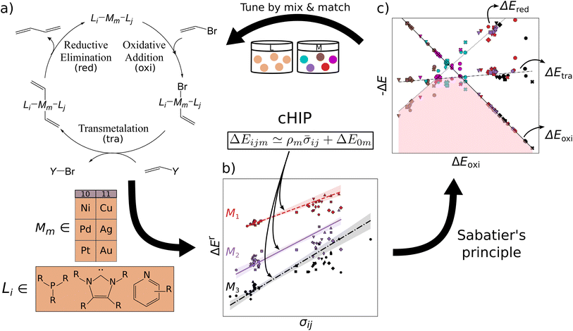
In this work, we introduce an approach that partitions the contributions of the metal and each ligand in organometallic catalysts using the SM reaction as a test case. This method facilitates computational ligand tuning through binding energy predictions and their implementation into volcano plots. We assess and propose methods for retrieving and combining individual ligand effects that ensure statistically stable calculations. The combining rule is integrated into a HIP model46,47 (Fig. 1b). Utilizing a dataset of 25k oxidative addition relative binding energies, we also investigate the performance of this combination rule-enhanced HIP model (cHIP) as a baseline for Δ-ML,56 which learns residuals and further mitigates excessive data needs. Subsequently, we show how the design flexibility afforded by cHIP can be used to expand a second, smaller catalyst dataset, DB2, into DB3 and conduct screening (Fig. 1c).
2. Methods and computational details
2.1 HIP model
In the context of homogeneous catalysis, assessing the binding free energies between catalysts and substrates at each step of the catalytic cycle aids in screening, as shown by Busch et al.57 and utilized later in this work. Herein, we multiply the Hammett equation32,33 by −RT, where R is the ideal gas constant and T is the temperature, to approximate changes in binding energy as a simple product, | (1) |
Although empirical σ values for common substituents in the ionization of benzoic acid derivatives can be found in the literature, such parameters are absent for many ligands pertinent to homogeneous catalysis. Furthermore, caution is warranted when assuming the transferability of these values for chemistries of different natures.58 Note that in eqn (1), the necessity of establishing a ligand as a reference is due to the ligand space being larger compared to metals. The HIP model, as introduced by Bragato et al.,46,47 enables the investigation of similar reactions by extracting linear scaling factors between them and eliminating reliance on external references. It comprises the following 3 steps:
| ΔElm ≃ ρmσl + ΔE0m | (2) |
Furthermore, the binding energy changes can be stored in a matrix M, where X is the number of metals and Y is the number of ligand groups,
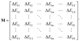 | (3) |
For each column, the internal reference ΔE0m is defined as its median.
 , or
, or| cmnρn − ρm = 0 | (4) |
c
mn
is computed as the slope of the line of best fit between all ΔElm and ΔEln for 1 ≤ l ≤ Y (see Fig. 2). The procedure adopts Theil–Sen regression,59,60 evaluating the median of  pairwise slopes (ΔElm – ΔEkm)/(ΔEln − ΔEkn) for 1 ≤ l < k ≤ Y. Ordering the slopes in a list S, we get
 | (5) |
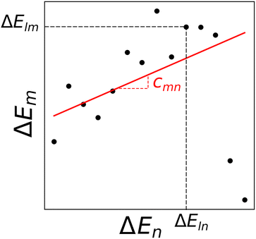 | ||
| Fig. 2 Binding energies for complexes with metals m and n. Each point represents a distinct ligand combination. The regression line, obtained through Theil–Sen regression,46,59,60 has a slope representing the median of all pairwise slopes. | ||
This method offers the advantage of being more robust towards outliers, but it scales quadratically with the number of data points.Accounting for all permutations of m and n, m ≠ n, eqn (4) yields an overdetermined system of linear equations Cρ = 0 which can be used to solve for ρs. A comprehensive description of this matrix is provided in the supplementary information† section (SI).
 | (6) |
2.2 Combination rule
In cases where the σs of individual substituents are known, one can assume that an additive combination rule can be used to retrieve the effects of any combination of them. This idea was generalized and confirmed already in 1953 by Jaffé who compiled overwhelming evidence in support of this effect.48 We note for this work that conversely individual ligand contributions can also be inferred as soon as sufficiently many σs for combinations of substituents (groups) are known. We have exploited the latter idea to first quantify σs for individual ligands via linear regression and to subsequently add them for estimating σs of novel ligand combinations.In order to reconfirm the validity of this approach we revisited the previously published data. In particular, the effect of a group of ligands l is approximated as
 | (7) |
![[small sigma, Greek, macron]](https://www.rsc.org/images/entities/i_char_e0d2.gif) i by solving the system of equations
i by solving the system of equationsD![[small sigma, Greek, macron]](https://www.rsc.org/images/entities/b_char_e0d2.gif) = σl = σl | (8) |
![[small sigma, Greek, macron]](https://www.rsc.org/images/entities/i_char_e0d2.gif) is the vector of single substituent effects that can be solved via the linear least squares method.
is the vector of single substituent effects that can be solved via the linear least squares method.
Results on display in Fig. 3 confirm our expectation that σs of combinations are additive in σs of single ligands. These experimental constants were obtained from studies on the hydrolysis of phosphonium salts,61 alcoholysis of isocyanates,62 and various reactions involving benzoic acids.48 The datasets encompassed di- and trisubstituted compounds featuring small substituents such as Cl, CH3, OCH3, NO2, etc., each with established Hammett parameters. Furthermore, note that the sums of parameters obtained through linear regression (Fig. 3b) are consistently closer to the experiments than the sums of Hammett parameters. This enhanced accuracy of the least squares method, presumably due to improved regularization and balancing, suggests its capability to robustly account for environment-specific synergistic effects, typically absent within the arbitrarily selected experiments resulting in the initial Hammett parameters. We also report the performance of other combination rules in the ESI,† which revealed less accuracy than the additive rule.
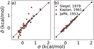 | ||
Fig. 3 Test of combination rule for experimentally obtained substituent parameters describing reactions of various chemistries (see text) published decades ago by Siegel,61 Kaplan,62 Jaffé.48 Substituent constants (![[small sigma, Greek, macron]](https://www.rsc.org/images/entities/i_char_e0d2.gif) ) were obtained by (a) summing published σ, and (b) after linear regression for each of the three published sets (this work). ) were obtained by (a) summing published σ, and (b) after linear regression for each of the three published sets (this work). | ||
For estimating relative binding energies to catalyst complexes in the SM coupling reaction we have first applied eqn (8) to ligand pairs using the σs obtained from HIP as σl. Then, cHIP predictions, ΔEc, can be obtained for any ligand pair ij and catalyst metal m via
ΔEijm ≃ ΔEcijm = ρm![[small sigma, Greek, macron]](https://www.rsc.org/images/entities/i_char_e0d2.gif) ij + ΔE0m = ρm(σi + σj) + ΔE0m ij + ΔE0m = ρm(σi + σj) + ΔE0m | (9) |
2.3 Δ-ML
To compare the above model to existing ML methods, we adopted an ML approach with Hammett to yield learning curves by fitting Hammett parameters to a growing training set and testing on fixed out-of-sample data. To obtain predictions for all data points, the data was divided into 5 folds, and each was used as a test set once while training on the 4 others. Due to varied training set sizes in the cHIP model, certain ligand combinations present in the test set might be absent from the training sets, especially with smaller training sets. Hence, a categorical regression using one-hot encoding was employed to estimate σ values for unknown ligands from known ones.46 Ligand constants from this step were used only in cases where they could not be estimated during training.The cHIP results served as a baseline for Δ-ML with KRR.56 KRR, a supervised ML technique initially introduced in chemistry for learning molecular atomization energies,63 maps data from the input space to a feature space and calculates the dot product of the transformed vectors. The mapped data in this case are the representations, which contain information derived from the molecular structure. For a given set of N training instances, the corrected predictions after Δ-ML are obtained using
 | (10) |
 | (11) |
 | (12) |
| α = (K + λI)−1y | (13) |
2.4 Datasets
Two datasets, both containing relative binding energies relative to the formation of 1,3-butadiene depicted in Fig. 1a, were used in this work, as summarized in Table 1.| Purpose | Catalyst structure | Metals | # of ligands | Reaction steps | # of data entries | Data origin | |
|---|---|---|---|---|---|---|---|
| DB1 | Test combination rule | L i − Mm − Lj | Ni, Pd, Pt, Cu, Ag, Au | 91, see ESI | Oxidative addition | 25![[thin space (1/6-em)]](https://www.rsc.org/images/entities/char_2009.gif) 116 116 |
7054 from DFT20 + 18![[thin space (1/6-em)]](https://www.rsc.org/images/entities/char_2009.gif) 062 from KRR using MBDF and Laplacian kernel (this work) 062 from KRR using MBDF and Laplacian kernel (this work) |
| DB2 | Catalyst discovery | L i − Mm − Li | Ni, Pd, Pt, Cu, Ag, Au | 16, see ESI | Oxidative addition, transmetalation, reductive elimination | 276 | 276 from DFT (92 per reaction step)64 |
| DB3 | Novel catalysts | L i − Mm − Lj | Ni, Pd, Pt, Cu, Ag, Au | 16, see ESI | Oxidative addition, transmetalation, reductive elimination | 720 | cHIP (this work) |
The first one, referred to as Database 1 (DB1) was obtained from ref. 20. It contains a total of 91 ligands of types phosphines (P), N-heterocyclic carbenes (NHC), pyridines (Py), and other common ligands (Other). Their chemical structures are provided in the SI. Those ligands were combined with six transition metals (Ni, Pd, Pt, Cu, Ag, and Au) to form catalysts having the structure Li − Mm − Lj, where Li and Lj are ligands and Mm is a metal, spanning a total set of 25![[thin space (1/6-em)]](https://www.rsc.org/images/entities/char_2009.gif) 116 compounds. It contained relative binding energies relative to the oxidative addition step in the SM C–C cross-coupling reaction depicted in Fig. 1a for 4186 Li – Lj combinations, each coupled with all 6 metals. The distributions of the energies by metal and by ligand type combinations, shown in Fig. S1 and S2† respectively, primarily show that the energies are more strongly correlated with metals than with ligands.A subset of 7054 geometries in DB1 was optimized using the AiiDA automated platform65 at the B3LYP-D3/3-21G66,67 level of theory for the Ni, Pd, Cu, and Ag complexes, and B3LYP-D3/def2-SVP68 for the Pt and Au complexes in Gaussian09.69 Subsequently, B3LYP-D3/def2-TZVP70 single-point calculations were performed. The remaining 18
116 compounds. It contained relative binding energies relative to the oxidative addition step in the SM C–C cross-coupling reaction depicted in Fig. 1a for 4186 Li – Lj combinations, each coupled with all 6 metals. The distributions of the energies by metal and by ligand type combinations, shown in Fig. S1 and S2† respectively, primarily show that the energies are more strongly correlated with metals than with ligands.A subset of 7054 geometries in DB1 was optimized using the AiiDA automated platform65 at the B3LYP-D3/3-21G66,67 level of theory for the Ni, Pd, Cu, and Ag complexes, and B3LYP-D3/def2-SVP68 for the Pt and Au complexes in Gaussian09.69 Subsequently, B3LYP-D3/def2-TZVP70 single-point calculations were performed. The remaining 18![[thin space (1/6-em)]](https://www.rsc.org/images/entities/char_2009.gif) 062 energies were predicted by us using a KRR model trained on the DFT energies using the Many-Body Distribution Functionals (MBDF)27 representation and a Laplacian kernel, providing full coverage of all ligand–metal combinations at a reduced computational cost. Three other representations and kernel combinations were built for comparison, namely Coulomb Matrix15 and Bag of Bonds (BoB)26 with a Laplacian kernel, and Spectrum of London and Axilrod–Teller–Muto potential (SLATM)25 with a Gaussian kernel, hence reproducing Meyer et al.'s work.20 As shown in Fig. 4, the comparison leads to the conclusion that MBDF, with the Laplacian kernel, yields the best result.
062 energies were predicted by us using a KRR model trained on the DFT energies using the Many-Body Distribution Functionals (MBDF)27 representation and a Laplacian kernel, providing full coverage of all ligand–metal combinations at a reduced computational cost. Three other representations and kernel combinations were built for comparison, namely Coulomb Matrix15 and Bag of Bonds (BoB)26 with a Laplacian kernel, and Spectrum of London and Axilrod–Teller–Muto potential (SLATM)25 with a Gaussian kernel, hence reproducing Meyer et al.'s work.20 As shown in Fig. 4, the comparison leads to the conclusion that MBDF, with the Laplacian kernel, yields the best result.
The second and smaller dataset (Database 2 or DB2) was obtained from ref. 64 and provides relative binding free energies for all 3 intermediate steps depicted in Fig. 1a. The values include unscaled enthalpies and vibrational entropy contributions. It contains symmetrical complexes, composed of the same 6 metals as in the first dataset and 16 ligands. 10 out of those 16 ligands were also present in the first one, and the energies of 4 Cu-based complexes were missing, yielding only 92 complexes per reaction step. The geometries of these complexes were optimized using M06/def2-SVP68,71,72 in Gaussian09 (ref. 69) while accounting for solvation in tetrahydrofuran using the implicit SMD model.73
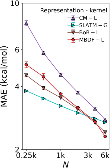 | ||
| Fig. 4 Test of ML model used to augment the DFT data in DB1 (Table 1). Learning curves (test error of relative binding energies vs. training set size) for oxidative addition for different ML methods. L: Laplacian kernel, G: Gaussian kernel. The augmentation was done using the MBDF-based model trained on all 7054 DFT training points published in ref. 20. | ||
3. Results and discussion
3.1 cHIP on oxidative addition (DB1)
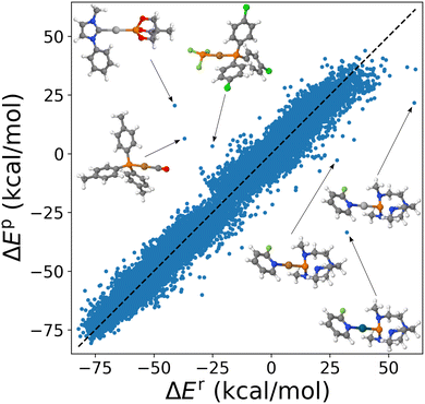
Application of the combination rule to 91 substituent specific σs within cHIP (eqn (9)) resulted in a mean absolute error (MAE) of ∼3.4 kcal mol−1 for DB1. We note that the naive HIP model (eqn (2)), which accounts for changes in binding using 912/2 = 4186 global σs, reached a MAE of ∼2.5 kcal mol−1. This increase of MAE from HIP to cHIP is expected due to the decrease in dimensionality from the additional layer of approximation introduced by estimating the combined ligand contributions as the sum of individual ones. Corresponding scatter plots of 25![[thin space (1/6-em)]](https://www.rsc.org/images/entities/char_2009.gif) 116 model predictions versus reference data numbers (used for fitting) are shown in Fig. 5 and S3† for cHIP and HIP, respectively. Such predictive power, only on the order of a few percentage points of the range of the property (see Fig. S1†) is promising. We note that it is on par with popular density functional approximations, as well as with previous HIP results obtained for estimating activation energies in SN2 reactions.46
116 model predictions versus reference data numbers (used for fitting) are shown in Fig. 5 and S3† for cHIP and HIP, respectively. Such predictive power, only on the order of a few percentage points of the range of the property (see Fig. S1†) is promising. We note that it is on par with popular density functional approximations, as well as with previous HIP results obtained for estimating activation energies in SN2 reactions.46
Note how in Fig. 5, no skewing is observed (see also the error distribution curve per metal in Fig. S5†). As displayed as insets, outliers correspond to varying metals. However, they all have in common that there is one P ligand. Furthermore, all underestimated outliers correspond to catalysts that share the same ligands, proazaphosphatrane, and 2-fluoropyridine.
Most outliers of the cHIP model (Fig. 5) were also outliers already for the HIP model (Fig. S3†). This suggests that, beyond the decrease in dimensionality caused by the combination rule, these shortcomings are likely to be caused by the Hammett equation's inadequacy in describing those specific ligands. This inadequacy can only be partly explained by steric hindrance since the dataset also comprised several bulky NHC ligands which were not outliers. We also note that since many systems used for fitting are sterically hindered, some steric effects could be included in the cHIP parameters.
Performing the regression on subsets according to the categories of each of its ligands further improved the prediction accuracy. In Fig. 8, all the cHIP models fitted on the subsets had lower errors than the full dataset model. These observations agree with the statement that a Hammett correlation occurs between closely related species.35 They are also in line with the fact that regression is more difficult the higher the dimensionality.74 As such, cHIP promises to be a useful model for combinatorially scaling spaces (the combinations of ligands in this case) with low-dimensional chemistry-specific properties, and where limited training instances are available.
The individual σs were retrieved by applying the combination rule on the HIP predictions to produce the Hammett plot in Fig. 6. Moreover, the distinct clustering of complexes by their central metal and the linear trends in Fig. 6 validate the adequacy of the partitioning of ρ and σ.
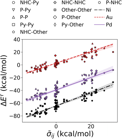 | ||
| Fig. 6 Demonstration of cHIP. Oxidative addition relative binding energies (DB1, see Table 1) are shown as a function of averaged σ obtained from cHIP. For the sake of simplicity, only 5 examples from each ligand type combination (given as legends) are plotted for each of the three metals. Lines correspond to cHIP predictions. | ||
A closer look at the calculation of the individual σs for DB1 in Fig. 7 revealed a MAE of 2.5 kcal mol−1 between the σs from HIP and cHIP. While an overestimation is usually observed with the additive rule when summing existing Hammett parameters,48,75 we have circumvented this by fitting those parameters with linear regression. The corresponding error distribution of cHIP σs (inset of Fig. 7) illustrates the welcome absence of any bias.
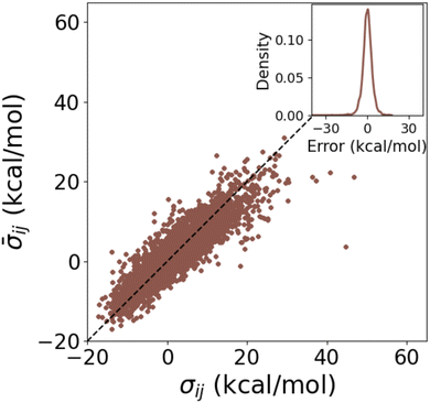 | ||
Fig. 7 Test of combination rule for individually obtained substituent parameters using DB1 (Table 1). Averaged ![[small sigma, Greek, macron]](https://www.rsc.org/images/entities/i_char_e0d2.gif) (cHIP on DB1) vs. reference σ (HIP on DB1) for combinations of ligands i and j. The inset shows the corresponding error distribution. (cHIP on DB1) vs. reference σ (HIP on DB1) for combinations of ligands i and j. The inset shows the corresponding error distribution. | ||
3.2 Δ-ML
When regressing cHIP onto the entire DB1 (DFT + ML augmented instances), the prediction error ceases to improve, leveling off at ∼4 kcal mol−1 (see Fig. 8). Note how the offset of the plateau is located at ∼1k training instances which roughly corresponds to the total number of parameters to fit in eqn (9). While several physics-based representations, such as CM,15 global MBDF,27 BoB,26 or SLATM,25 enable KRR models to systematically improve with training set size (see Fig. 4), DB1 does not contain sufficient DFT instances to allow for convergence lower than 2 kcal mol−1. Understanding catalytic yield relies on thermodynamic quantities for homogeneous catalysis,57 where equilibrium constants exhibit exponential scaling with free energy differences, underscoring the significance of predicting such changes with chemical accuracy (1 kcal mol−1). Encouragingly, when combining cHIP as a baseline with a machine-learned correction, Δ-ML, the resulting learning curve on DB1 continues to improve with training set size, reaching a MAE corresponding to chemical accuracy for ∼20k training instances. The systematically decreasing standard deviations of the prediction errors in the learning curves are equally promising, and can be attributed to an increasingly slimmer error distribution, similar to previously noted trends for ML models of formation energies of crystals.76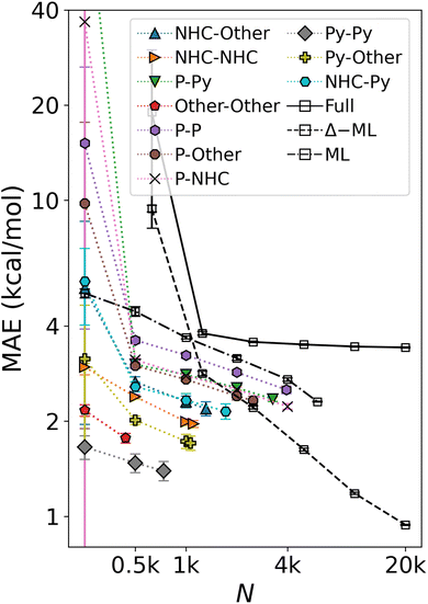 | ||
| Fig. 8 Mean absolute error of predicting relative binding energies in the oxidative addition step as a function of training set size. Errors of cHIP models on subsets (colored) and full DB1 (Table 1) plateau rapidly. ML corresponds to the KRR/MBDF line shown in Fig. 4. Δ-ML model trained on DB1 results with cHIP baseline results in lower offset and enables convergence to chemical accuracy. Error bars indicate standard deviations. | ||
3.3 Catalyst discovery (DB2)
We have studied the utility of cHIP in catalyst discovery through volcano plots. For homogeneous catalysis, such plots are built by establishing linear scaling relationships between all the intermediate steps against a reference step57 using a descriptor such as the catalyst–substrate binding free energy. This allows for identifying an ideal range of energies in which only certain catalysts fall, aligning with Sabatier's principle.77 This strategy provides a way of screening potential catalysts without kinetic data. DB2 was used in this phase as it contains relative binding free energies for all 3 steps.The fitting of HIP to the entire dataset, illustrated in Fig. 9a, resulted in MAEs consistently below 3.5 kcal mol−1 for all steps. Leveraging the effects of 16 single ligands, cHIP successfully predicted the ligand effects of 120 new ligand combinations. Pairing these with each of the 6 metals, we predicted relative binding free energy changes for an additional 720 catalysts, reported in DB3.
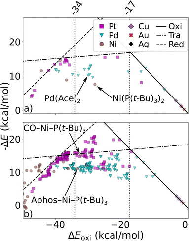 | ||
| Fig. 9 Volcano plot: negative relative binding free energies of each step are plotted as a function of that of the oxidative step (oxi). Ideal catalysts lie at the top of the volcano and vertical lines represent the ideal range as identified by Busch et al.64 (a) catalysts sourced from DB2 (Table 1). (b) novel catalysts predicted using cHIP, the 198 most interesting catalysts lie in between the two intersections of the transmetalation with either oxidative addition or reductive elimination. Two inexpensive (Ni-based) catalysts in the optimal regime are indicated by arrows. | ||
As depicted in Fig. 9b, 198 of the new catalysts lie at the top of the predicted volcano plot. Among these, 145 displayed oxidative addition relative binding free energies ranging from −34.0 to 17.0 kcal mol−1, previously identified as an optimal range by Busch et al.64 This combinatorial approach revealed several Ni-based catalysts approaching the top of the volcano after ligand tuning, despite the initially strong-binding nature of Ni. The discovery of these catalysts, derived from a metal that is more cost-effective and earth-abundant than the prominent Pd, is particularly attractive and has been actively explored in the field over the past decade.30,78 When considering the cost of the ligands, the most cost-effective catalyst identified by cHIP is Aphos-Ni-P(t-Bu)3, representing about 67% of the cost of the least expensive catalyst found in DB2, Pd(Ace)2, based on ligand and metal prices provided by Sigma-Aldrich.79 Similar phosphine ligands for Ni catalysts have been reported in literature such as ProPhos80 or P(Cy)3.81
Notably, the model was able to capture a reasonable trend across both datasets, despite DB1 lacking solvent effects and DB2 incorporating implicit solvation. This suggests that the cHIP model could potentially make equally reliable predictions when trained on datasets that include explicit solvation effects.
4. Conclusion
Our study demonstrates the efficacy of employing an additive combination rule with Hammett's equation for computational catalyst discovery. We have exemplified its applicability to the prediction and analysis of organometallic complexes relevant to the catalysis of the Suzuki–Miyaura (SM) cross-coupling reaction. We exploit fitted Hammett parameters obtained from linear least squares regression across all available ligand combinations, surpassing the prediction performance of published Hammett parameters. Due to its simplicity, this approach offers significant computational advantages, obviating the need for geometric coordinates or extensive computing resources, therefore serving as a quick yet useful screening tool. It also proves valuable when dealing with smaller chemical compound subspaces. Furthermore, our findings illustrate its utility as a baseline for Δ-ML, reaching predictive power with chemical accuracy. The ability to separate ligand pair effects into single ligand effects facilitates the exploration of larger catalyst spaces and ligand tuning. This was demonstrated for a dataset comprising symmetrical catalysts created through the combination of 16 ligands and 6 metals. Our model identified 145 new catalyst candidates for the SM reaction, including some based on Ni implying potentially substantial cost savings. For example, we identified the phosphine ligand-based Ni catalyst, Aphos-Ni-P(t-Bu)3, which seems to fall in line with other reported phosphine ligands. Future research directions will include further investigation of the effect of crowding and the specific environments on the ligand constants, aiming to elucidate the outliers in the model (phosphorus-containing ligands) and extend this approach to other catalysts and complexes with more than two ligands.Data availability
This study was carried out using publicly available data (structures and binding energies) from the Material Cloud at doi: https://doi.org/10.24435/materialscloud:2018.0014/v1 from ref. 20 and https://doi.org/10.24435/materialscloud:2019.0007/v3 from ref. 64. Supporting data are included in the article's ESI.† Scripts and additional data are available at https://github.com/dianarak/cHIP.git and doi: https://doi.org/10.5281/zenodo.13874311.Conflicts of interest
There are no conflicts to declare.Acknowledgements
We acknowledge the support of the Natural Sciences and Engineering Research Council of Canada (NSERC), RGPIN-2023-04853. O. A. v. L. has received funding from the European Research Council (ERC) under the European Union's Horizon 2020 research and innovation programme (grant agreement No. 772834). This research was undertaken thanks in part to funding provided to the University of Toronto's Acceleration Consortium from the Canada First Research Excellence Fund, grant number: CFREF-2022-00042. O. A. v.L. has received support as the Ed Clark Chair of Advanced Materials and as a Canada CIFAR AI Chair.References
- A. Pradal, S. Gladiali, V. Michelet and P. Y. Toullec, Chem.–Eur. J., 2014, 20, 7128 CrossRef CAS PubMed.
- M. T. Reetz, Angew. Chem., Int. Ed., 2008, 47, 2556 CrossRef CAS PubMed.
- E. Moulin, G. Cormos and N. Giuseppone, Chem. Soc. Rev., 2012, 41, 1031 RSC.
- R. Liu, X. Li and K. S. Lam, Curr. Opin. Chem. Biol., 2017, 38, 117 CrossRef CAS PubMed.
- K. D. Collins, T. Gensch and F. Glorius, Nat. Chem., 2014, 6, 859 CrossRef CAS PubMed.
- K. D. Shimizu, M. L. Snapper and A. H. Hoveyda, Chem.–Eur. J., 1998, 4, 1885 CrossRef CAS.
- E. S. Isbrandt, R. J. Sullivan and S. G. Newman, Angew. Chem., Int. Ed., 2019, 58, 7180 CrossRef CAS PubMed.
- C. A. Shepherd, A. L. Hopkins and I. Navratilova, Prog. Biophys. Mol. Biol., 2014, 116, 113 CrossRef CAS PubMed.
- S. Li, Y. Song, X. Liu and H. Li, Comb. Chem. High Throughput Screening, 2016, 19, 25 CrossRef CAS PubMed.
- A. Nandy, C. Duan, M. G. Taylor, F. Liu, A. H. Steeves and H. J. Kulik, Chem. Rev., 2021, 121, 9927 CrossRef CAS PubMed.
- J. R. Kitchin, Nat. Catal., 2018, 1, 230 CrossRef.
- B. Burger, P. M. Maffettone, V. V. Gusev, C. M. Aitchison, Y. Bai, X. Wang, X. Li, B. M. Alston, B. Li and R. Clowes, et al. , Nature, 2020, 583, 237 CrossRef CAS PubMed.
- B. Huang, G. F. von Rudorff and O. A. von Lilienfeld, Science, 2023, 381, 170 CrossRef CAS PubMed.
- F. Strieth-Kalthoff, F. Sandfort, M. H. Segler and F. Glorius, Chem. Soc. Rev., 2020, 49, 6154 RSC.
- M. Rupp, A. Tkatchenko, K.-R. Müller and O. A. von Lilienfeld, Phys. Rev. Lett., 2012, 108, 058301 CrossRef PubMed.
- D. T. Ahneman, J. G. Estrada, S. Lin, S. D. Dreher and A. G. Doyle, Science, 2018, 360, 186 CrossRef CAS PubMed.
- J. P. Reid and M. S. Sigman, Nature, 2019, 571, 343 CrossRef CAS PubMed.
- K. Jorner, A. Tomberg, C. Bauer, C. Sköld and P.-O. Norrby, Nat. Rev. Chem, 2021, 5, 240 CrossRef CAS PubMed.
- G. dos Passos Gomes, R. Pollice and A. Aspuru-Guzik, Trends Chem., 2021, 3, 96 CrossRef CAS.
- B. Meyer, B. Sawatlon, S. Heinen, O. A. von Lilienfeld and C. Corminboeuf, Chem. Sci., 2018, 9, 7069 RSC.
- O. Schilter, A. Vaucher, P. Schwaller and T. Laino, Digital Discovery, 2023, 2, 728 RSC.
- N. Miyaura, K. Yamada and A. Suzuki, Tetrahedron Lett., 1979, 20, 3437 CrossRef.
- N. Miyaura and A. Suzuki, Chem. Rev., 1995, 95, 2457 CrossRef CAS.
- A. Suzuki, Angew. Chem., Int. Ed., 2011, 50, 6722 CrossRef CAS PubMed.
- B. Huang and O. A. von Lilienfeld, Nat. Chem., 2020, 12, 945 CrossRef CAS PubMed.
- K. Hansen, F. Biegler, R. Ramakrishnan, W. Pronobis, O. A. von Lilienfeld, K.-R. Muller and A. Tkatchenko, J. Phys. Chem. Lett., 2015, 6, 2326 CrossRef CAS PubMed.
- D. Khan, S. Heinen and O. A. von Lilienfeld, J. Chem. Phys., 2023, 159, 034106 CrossRef CAS PubMed.
- J. Damewood, J. Karaguesian, J. R. Lunger, A. R. Tan, M. Xie, J. Peng and R. Gómez-Bombarelli, Annu. Rev. Mater. Res., 2023, 53, 399 CrossRef CAS.
- A. M. Chang, J. G. Freeze and V. S. Batista, Chem. Sci., 2019, 10, 6844 RSC.
- F.-S. Han, Chem. Soc. Rev., 2013, 42, 5270 RSC.
- R. Martin and S. L. Buchwald, Acc. Chem. Res., 2008, 41, 1461 CrossRef CAS PubMed.
- L. P. Hammett, Chem. Rev., 1935, 17, 125 CrossRef CAS.
- L. P. Hammett, J. Am. Chem. Soc., 1937, 59, 96 CrossRef CAS.
- H. H. Jaffé and H. L. Jones, in Advances in Heterocyclic Chemistry, Elsevier, 1964, vol. 3, pp. 209–261 Search PubMed.
- A. K. Chattopadhyay, A. Bhattacharyya and S. C. Lahiri, Z. fur Phys. Chem., 1976, 102, 151–158 CrossRef CAS.
- Z.-B. Dong, G. Manolikakes, L. Shi, P. Knochel and H. Mayr, Chem.–Eur. J., 2010, 16, 248 CrossRef CAS PubMed.
- R. W. Taft Jr, J. Am. Chem. Soc., 1953, 75, 4538 CrossRef.
- R. W. Taft Jr, J. Am. Chem. Soc., 1952, 74, 3120 CrossRef.
- R. W. Taft Jr, J. Am. Chem. Soc., 1952, 74, 2729 CrossRef.
- M. Charton, J. Am. Chem. Soc., 1975, 97, 1552 CrossRef CAS.
- M. Charton, J. Am. Chem. Soc., 1975, 97, 3691 CrossRef CAS.
- M. Charton, J. Org. Chem., 1976, 41, 2217 CrossRef CAS.
- A. Verloop, W. Hoogenstraaten and J. Tipker, Drug Des., 1976, 7, 165 Search PubMed.
- K. C. Harper, E. N. Bess and M. S. Sigman, Nat. Chem., 2012, 4, 366 CrossRef CAS PubMed.
- M. S. Sigman, K. C. Harper, E. N. Bess and A. Milo, Acc. Chem. Res., 2016, 49, 1292 CrossRef CAS PubMed.
- M. Bragato, G. F. von Rudorff and O. A. von Lilienfeld, Chem. Sci., 2020, 11, 11859 RSC.
- M. Bragato, G. F. von Rudorff, and O. A. von Lilienfeld, Occam's razor for ai: Coarse-graining Hammett inspired product ansatz in chemical space, arXiv, 2023, preprint, arXiv:2305.07010 [physics.chem-ph], DOI:10.48550/arXiv.2305.07010.
- H. H. Jaffé, Chem. Rev., 1953, 53, 191–261 CrossRef.
- A. K. Al-Matar and D. A. Rockstraw, J. Comput. Chem., 2004, 25, 660 CrossRef CAS PubMed.
- J. Delhommelle and P. Millié, Mol. Phys., 2001, 99, 619 CrossRef CAS.
- M. Fyta and R. R. Netz, J. Chem. Phys., 2012, 136, 124103 CrossRef PubMed.
- H. A. Lorentz, Ann. Phys., 1881, 248, 127–136 CrossRef.
- D. Berthelot, Compt. Rendus, 1898, 126, 15 Search PubMed.
- B. Fender and G. Halsey Jr, J. Chem. Phys., 1962, 36, 1881 CrossRef CAS.
- M. Waldman and A. T. Hagler, J. Comput. Chem., 1993, 14, 1077 CrossRef CAS.
- R. Ramakrishnan, P. O. Dral, M. Rupp and O. A. von Lilienfeld, J. Chem. Theory Comput., 2015, 11, 2087–2096 CrossRef CAS PubMed.
- M. Busch, M. D. Wodrich and C. Corminboeuf, Chem. Sci., 2015, 6, 6754 RSC.
- D. Pearson, J. Baxter and J. Martin, J. Org. Chem., 1952, 17, 1511 CrossRef CAS.
- H. Theil, Indag. Math., 1950, 12, 173 Search PubMed.
- P. K. Sen, J. Am. Stat. Assoc., 1968, 63, 1379 CrossRef.
- B. Siegel, J. Am. Chem. Soc., 1979, 101, 2265 CrossRef CAS.
- M. Kaplan, J. Chem. Eng. Data, 1961, 6, 272 CrossRef CAS.
- K. Hansen, G. Montavon, F. Biegler, S. Fazli, M. Rupp, M. Scheffler, O. A. von Lilienfeld, A. Tkatchenko and K.-R. Müller, J. Chem. Theory Comput., 2013, 9, 3404 CrossRef CAS PubMed.
- M. Busch, M. D. Wodrich and C. Corminboeuf, ACS Catal., 2017, 7, 5643 CrossRef CAS.
- G. Pizzi, A. Cepellotti, R. Sabatini, N. Marzari and B. Kozinsky, Comput. Mater. Sci., 2016, 111, 218 CrossRef.
- S. Grimme, J. Antony, S. Ehrlich and H. Krieg, J. Chem. Phys., 2010, 132, 154104 CrossRef PubMed.
- S. Grimme, S. Ehrlich and L. Goerigk, J. Comput. Chem., 2011, 32, 1456 CrossRef CAS PubMed.
- F. Weigend and R. Ahlrichs, Phys. Chem. Chem. Phys., 2005, 7, 3297 RSC.
- M. J. Frisch, G. W. Trucks, H. B. Schlegel, G. E. Scuseria, M. A. Robb, J. R. Cheeseman, G. Scalmani, V. Barone, G. A. Petersson, H. Nakatsuji, X. Li, M. Caricato, A. V. Marenich, J. Bloino, B. G. Janesko, R. Gomperts, B. Mennucci, H. P. Hratchian, J. V. Ortiz, A. F. Izmaylov, J. L. Sonnenberg, D. Williams-Young, F. Ding, F. Lipparini, F. Egidi, J. Goings, B. Peng, A. Petrone, T. Henderson, D. Ranasinghe, V. G. Zakrzewski, J. Gao, N. Rega, G. Zheng, W. Liang, M. Hada, M. Ehara, K. Toyota, R. Fukuda, J. Hasegawa, M. Ishida, T. Nakajima, Y. Honda, O. Kitao, H. Nakai, T. Vreven, K. Throssell, J. A. Montgomery Jr, J. E. Peralta, F. Ogliaro, M. J. Bearpark, J. J. Heyd, E. N. Brothers, K. N. Kudin, V. N. Staroverov, T. A. Keith, R. Kobayashi, J. Normand, K. Raghavachari, A. P. Rendell, J. C. Burant, S. S. Iyengar, J. Tomasi, M. Cossi, J. M. Millam, M. Klene, C. Adamo, R. Cammi, J. W. Ochterski, R. L. Martin, K. Morokuma, O. Farkas, J. B. Foresman, and D. J. Fox, Gaussiañ09 Revision D.01, Gaussian Inc., Wallingford CT., 2016 Search PubMed.
- F. Weigend and R. Ahlrichs, Phys. Chem. Chem. Phys., 2005, 7, 3297 RSC.
- Y. Zhao and D. G. Truhlar, Acc. Chem. Res., 2008, 41, 157 CrossRef CAS PubMed.
- Y. Zhao and D. G. Truhlar, Theor. Chem. Acc., 2008, 120, 215 Search PubMed.
- A. V. Marenich, C. J. Cramer and D. G. Truhlar, J. Phys. Chem. B, 2009, 113, 6378 CrossRef CAS PubMed.
- D. Lemm, G. F. von Rudorff and O. A. von Lilienfeld, Mach. Learn.: Sci. Technol., 2023, 4, 045043 Search PubMed.
- F. Bhasha Sayyed and C. H. Suresh, New J. Chem., 2009, 33, 2465–2471 RSC.
- F. A. Faber, A. Lindmaa, O. A. von Lilienfeld and R. Armiento, Phys. Rev. Lett., 2016, 117, 135502 CrossRef PubMed.
- P. Sabatier, La catalyse en chimie organique, librairie polytechnique, 1913.
- B. A. Baviskar, P. V. Ajmire, D. S. Chumbhale, M. S. Khan, V. G. Kuchake, M. Singupuram and P. R. Laddha, Sustainable Chem. Pharm., 2023, 32, 100953 CrossRef CAS.
- Millipore Sigma, https://www.sigmaaldrich.com/CA/en, accessed: 2024-03-08.
- J. Yang, M. C. Neary and T. Diao, J. Am. Chem. Soc., 2024, 146(9), 6360–6368 CrossRef CAS PubMed.
- H. Chen, Z. Huang, X. Hu, G. Tang, P. Xu, Y. Zhao and C.-H. Cheng, J. Org. Chem., 2011, 76, 2338 CrossRef CAS PubMed.
Footnote |
| † Electronic supplementary information (ESI) available. See DOI: https://doi.org/10.1039/d4dd00228h |
| This journal is © The Royal Society of Chemistry 2024 |

