Sensitivity analysis of planetary boundary layer parameterization on meteorological simulations in the Yangtze river delta region, China

Abstract

The planetary boundary layer (PBL) plays a crucial role in determining meteorological fields and the diffusion of atmospheric pollutants. Therefore, accurate PBL simulation is necessary for precise meteorological and air quality simulations, and the choice of PBL scheme significantly influences the accuracy of simulation results. In this study, we investigate the seasonal and diurnal variations of typical meteorological variables over the Yangtze River Delta (YRD) region by using the Weather Research and Forecasting (WRF) model using four different closure schemes. These closure schemes include two non-local closure schemes, i.e., Yonsei University (YSU) and Asymmetric Convective Model version 2 (ACM2), as well as two local closure schemes named Mellor–Yamada–Janjic (MYJ) and Mellor–Yamada Nakanishi and Niino (MYNN). By comparing observations and model inter-comparisons, we discuss the similarities and differences in simulated results among different PBL schemes. The results indicate that local closure schemes, i.e., MYJ and MYNN, generally produce more realistic simulations of meteorological parameters. MYNN performs best in summer with a mean bias (MB) of 0.41 °C for temperature and 0.44 m s⁻¹ for wind speed, while MYJ shows better results under stable conditions during winter with a MB of 0.64 °C for temperature and −5.76% for relative humidity. YSU is found to have less bias in PBL height during summer with the highest R up to 0.81, while MYJ outperforms the three other schemes with the least MB of 38 m (R = 0.65) in winter. Each PBL closure scheme, i.e., the MYJ and MYNN local closure schemes, may not accurately capture all physical processes, leading to performance variations, especially during transitional seasons and under specific diurnal conditions. Thus, it is important to note that each scheme has its strengths and weaknesses, and the selection of the most appropriate scheme should depend on the specific variables and scenarios under consideration.

---

Environmental significance

The planetary boundary layer (PBL) plays a crucial role in determining meteorological fields and the diffusion of atmospheric pollutants. It is of great significance to accurately predict the PBL height for precise meteorological and air quality simulations. However, different choices of PBL schemes may give quite different results of the PBL under various land surfaces and in different seasons. In this study, we comprehensively evaluated the seasonal and diurnal variations of typical meteorological variables over the Yangtze River Delta (YRD) region by using the Weather Research and Forecasting (WRF) model using four major closure schemes. The results will be helpful for the air quality modellers.

1 Introduction

The planetary boundary layer (PBL) is an important component in air quality simulations as it affects the transport and dispersion of atmospheric pollutants. Turbulent motions within the PBL are responsible for the exchange of heat, moisture, and momentum between the Earth's surface and the atmosphere.¹ This exchange is dependent on the thermodynamic state of the PBL, which needs to be accurately characterized for proper representation in meteorological models. The selection of a suitable PBL scheme is crucial as it can significantly impact the accuracy of the simulated meteorological parameters, including wind speed, humidity, and boundary layer height, which in turn affect the simulation of air pollutant concentrations.^2–5 The uncertainties in the configurations of PBL scheme parameterization have substantial influence on simulation errors and biases in mesoscale models.⁶ Therefore, a robust characterization of the PBL in meteorological models is essential for accurate air quality simulations.

The sensitivity of different PBL schemes is often closely related to meteorological and geographical environments.^7–12 Previous studies have investigated the effects of various PBL schemes on simulated meteorological fields and evaluated the suitability of specific schemes for different geographical regions.^13–18 For instance, by using the 5th generation mesoscale model (MM5), Zhang and Zheng¹⁹ showed that the Blackadar (BLK) scheme performed better in the prediction of the daily cycle of temperature and surface wind speed during a mid-summer simulation in the United States. Another study by Sanjay²⁰ indicated that though the Troen–Mahrt (TM) scheme coupled to the land surface scheme generally performed better than BLK coupled to a simple soil slab model, it still tended to underestimate the humidity in the boundary layer under clear air conditions in northwest India. Kwun et al.²¹ found that the wind speed obtained from Weather Research and Forecasting (WRF) coupled with the Yonsei University (YSU) and Mellor–Yamada–Janjic (MYJ) schemes during a typhoon was more consistent with observations. By quantifying the meteorological elements simulated by four PBL schemes in the WRF model, Xie et al.²² showed that the PBL height (PBLH) simulated by the MYJ and Bougeault and Lacarrère (BouLac) schemes was higher than that simulated by the YSU and ACM2 schemes. Arregocés et al.¹³ simulated key meteorological variables over northern Colombia during the dry season in 2016, highlighting the non-local YSU scheme's overall performance and the local MYNN scheme's accuracy in specific variables.

Although various studies have investigated the impact of different parameterization schemes on the accuracy of simulated meteorological fields, their analyses have generally been limited to short time periods or focused on specific weather events. For instance, previous studies indicate that the YSU (or ACM2) scheme is suitable for daytime calculations, while its efficacy might differ during nighttime periods or under different seasonal conditions.^23–25 Moreover, a single PBL scheme may not be appropriate for annual simulations due to the seasonal variations of different parameterization schemes.^3,26–28 Therefore, it is crucial to consider temporal variations when selecting an optimal PBL scheme.

The Yangtze River Delta (YRD) region, situated in the north marine monsoon subtropical climate zone of southeast China, is a rapidly developing urban cluster in the country. In recent years, the region has suffered from severe air pollution issues,^29,30 attributed to a combination of unfavorable meteorological conditions and high anthropogenic emissions. The topography of the YRD region is diverse, mainly comprising plains in the north and east with mountains in the west and south, and the eastern region is adjacent to the sea. The weather in the YRD is generally warm and humid during summer, while the winter is cool and dry. Synoptic circulation conditions, such as the western Pacific subtropical high and the tropical cyclone system, can significantly affect the monsoon circulation, typhoon tracks, and moisture transport in the region.^31,32 Hence, it is crucial to accurately predict meteorological conditions to enable reliable air quality simulations and better forecast air pollution changes. This study aims to examine the performance of WRF-simulated meteorological conditions associated with different turbulence parameterization schemes in the YRD region, with a focus on their seasonal variability, discrepancies, and effectiveness. Four commonly used PBL schemes, i.e., YSU, ACM2, MYJ, and MYNN, are evaluated for reproducing the observed meteorological variables, PBL thermodynamical structure, and turbulent flux. We further assess the applicability of these PBL schemes in different seasons. The findings of this study can significantly improve air quality simulations and facilitate air pollution research.

2 Methodology

2.1 WRF configurations

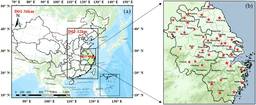
Weather Research and Forecasting (WRF) version 4.0 is utilized in this study. Three nested domains are configured with spatial resolutions of 36 km, 12 km, and 4 km, respectively (Fig. 1a and Table 1). The first domain (D01) covers most of East Asia and part of Southeast Asia, while the second domain (D02) covers eastern China. The third domain (D03) is focused on the entire Yangtze River Delta (YRD) region, which includes Shanghai metropolitan, Jiangsu province, Zhejiang province, and Anhui province, with a total of 41 cities. The spatial terrain elevation in D03 (Fig. 1b) ranges from about 25 m in the eastern, northern, and northeastern parts to about 1200 m in the western, southwestern, and southern parts of the domain, with a majority of the YRD showing an elevation below 50 m above sea level. The study uses 39 vertical levels with a model top set at 50 hPa. As listed in Table 1, the vertical resolution comprises 39 levels (η = 1.000, 0.9975, 0.995, 0.992, 0.989, 0.986, 0.983, 0.98, 0.976, 0.97, 0.961, 0.951, 0.94, 0.928, 0.916, 0.902, 0.889, 0.875, 0.85, 0.82, 0.78, 0.74, 0.7, 0.66, 0.62, 0.58, 0.54, 0.5, 0.45, 0.4, 0.35, 0.3, 0.25, 0.2, 0.15, 0.1, 0.06, 0.027, and 0) with 19 full η levels below 850 hPa. The corresponding geopotential height (GPH) of each level is calculated by using the following formula:

gmp = (PH + PHB)/9.81-HGT,

where the geopotential height (PH), base-state geopotential height (PHB) and terrain height (HGT) are the variables in the output of WRF. Thus, the 19 levels below 850 hPa are approximately 0, 21, 43, 69, 95, 121, 147, 173, 208, 261, 340, 430, 529, 638, 748, 869, 1000, 1132, and 1373 m. The height of the bottom level is very close to 0 m and always included in the planetary boundary layer. The minimum of the PBLH modelled with four schemes at Fuyang station is listed in the Table S2,† indicating that the percentage with the PBL height lower than the surface layer is small.

Fig. 1 Three nested modeling domains for the WRF model (a) and administrative divisions of 41 cities in the YRD region (b). (Blue triangle represents the radiosonde station at Fuyang; red stars represent locations of the surface meteorological observation sites).

Table 1 Configuration of the WRF model for the evaluation of PBL schemes in the YRD

Dynamics	Non-hydrostatic description
Study period	July and November in 2018
Resolution	D01: 36 × 36 km; D02: 12 × 12 km; D03: 4 × 4 km
Area cover	26.6°–35.1 °N, 114.9°–123.0 °E
Vertical resolution	39 vertical levels (η = 1.000, 0.9975, 0.995, 0.992, 0.989, 0.986, 0.983, 0.98, 0.976, 0.97, 0.961, 0.951, 0.94, 0.928, 0.916, 0.902, 0.889, 0.875, 0.85, 0.82, 0.78, 0.74, 0.7, 0.66, 0.62, 0.58, 0.54, 0.5, 0.45, 0.4, 0.35, 0.3, 0.25, 0.2, 0.15, 0.1, 0.06, 0.027, and 0 from bottom to top at 50 hPa)

---

The initial and lateral boundary conditions are based on the 6-hour Global Final Analysis data (1.0° × 1.0° resolution) provided by the National Center for Environmental Prediction (NCEP) and the National Center for Atmospheric Research (NCAR). The main physical parameterization schemes include the Lin microphysics scheme,³³ the NOAH land surface scheme,³⁴ the Kain–Fritsch (KF) cumulus parameterization (only used in D01 and D02),³⁵ the Rapid Radiative Transfer Model shortwave radiation scheme and the Rapid Radiative Transfer Model longwave radiation scheme.³⁶

To capture the diverse meteorological characteristics of the YRD region, we conducted simulations for both summer (July 2018) and winter (November 2018) periods. These months were specifically chosen for their typical representation of hot and humid summer conditions and cold and dry winter conditions, respectively. Notably, the WRF model is specifically configured as a regional climate model. This study has employed it to conduct continuous monthly simulations to investigate regional climate dynamics rather than deploying it in a conventional weather prediction mode with daily initializations. The WRF model in this study runs for 6 days at a time without the need for restarting or re-initializing during the simulation period. The FDDA feature is enabled, with the model performing data assimilation every 6 hours. This improves the simulation accuracy and allows us to capture the seasonal variation of the regional climate system, providing valuable insights into its behavior under different atmospheric conditions. As emphasized in the study of Ma et al.,¹⁰ enhanced representation of surface morphology and momentum transport coefficients is crucial for better simulations over complex terrains. The land use data of the YRD utilized in WRF were updated by interpreting from Landsat satellite imageries in 2018 and the replaced terrain covers were detailed in our previous study.³⁷ We verified that the meteorological conditions in 2018 were consistent with the average conditions from 2010–2020, with an average annual temperature, relative humidity, and precipitation of 17.5 °C (compared to a decade average of 17.3 °C), 74.3% (73.8% for the decade), and 1495.2 mm (1545.8 mm for the decade), respectively. These conditions confirm that 2018 was representative of the general meteorological patterns in the YRD region. Additionally, previous studies have indicated that July and November are suitable months to represent summer and winter seasons in the YRD region, further strengthening our choice.^{11,30,38–42} We excluded the initial 72 hours of each month for spin-up, and focused our analysis on the hourly outputs of the model.

2.2 PBL scheme

The original closed equation set fully describes the turbulent motion in the PBL. However, the addition of new variables representing the variance causes the equations to become unclosed. To address this, turbulence modelling is used to approximate the unknown quantity.⁴³ One major component of the turbulence processes is whether a local or non-local mixing approach is employed. Local closure schemes obtain the turbulent fluxes at each grid using the mean atmospheric variables at that model grid, while non-local closure schemes use the mean values from multiple vertical levels and profiles of the convective boundary layer to determine variables.⁴⁴ In this study, two local closure schemes (MYJ and MYNN) and two non-local closure schemes (YSU and ACM2) are considered in the Weather Research and Forecasting (WRF) model, as they represent the most commonly used schemes in various applications.^45–50

The YSU scheme is a first-order non-local closure scheme that has been revised from the Medium-Range Forecast (MRF) scheme. It has shown significant improvement through incorporating an explicit term to account for the entrainment process. Meanwhile, the ACM2 scheme is a hybrid first-order scheme that combines the ACM1 and local eddy diffusion by introducing the f_conv parameter.⁵¹ Thereinto, the f_conv parameter is adjusted by using the PBLH and Monin–Obukov length scale instead of using extreme values (f_conv = 1 or 0) for the ACM1 non-local scheme or local eddy diffusion. This scheme is particularly suitable for predicting humidity, winds, and trace chemical mixing ratios in the boundary layer scheme as it better represents the shape of the vertical profiles. Additionally, the ACM2 scheme tends to result in a deeper convective boundary layer due to its larger critical bulk Richardson number (R_i).⁵²

Local closure schemes, such as the MYJ scheme,⁵³ diagnose the vertical mixing process in the PBL and free atmosphere by forecasting the turbulent kinetic energy (TKE). Notably, in the MYJ scheme, the upper limit of the main length scale depends on the TKE and the shear stress of the buoyancy and driving flow. Compared to other schemes, the MYJ scheme produces a moister, cooler, and less mixed PBL.⁵⁴ Another local closure scheme, the MYNN scheme,⁵⁵ is also a one-and-a-half order scheme based on the Mellor–Yamada prognostic TKE scheme. To overcome the biases of both underestimated TKE and insufficient growth of the convective boundary layer, MYNN incorporates the effects of buoyancy in the diagnosis of the pressure covariance terms. It also uses closure constants in the stability functions and mixing length formulations based on large eddy simulation results rather than observational datasets.^56–58

We conducted WRF simulations using the aforementioned four PBL schemes while keeping other inputs and parameters consistent. This approach allowed us to reveal the impacts of different PBL schemes on meteorological simulations in a complex region such as the Yangtze River Delta (YRD) across various seasons.

2.3 Meteorological and radiosonde observation data

We compared the simulated 2 m surface temperature (T₂), 10 m wind speed (WS₁₀), and 2 m relative humidity (RH₂) with hourly observations from 41 meteorological stations in each city of the Yangtze River Delta (YRD) region. Hourly data were downloaded from the China National Meteorological Information Center. The locations of the 41 meteorological stations in the YRD region are indicated in Fig. 1, with the corresponding surface land use types detailed in Table S1.† We evaluated the meteorological variables based on the mean bias (MB), root mean square error (RMSE), normalized mean bias (NMB), normalized mean error (NME), and correlation coefficient (R):where M and O refer to the simulated and observed meteorological values, respectively. N represents the number of data pairs.

We conducted radiosonde measurements using an L-band radiosonde with a vertical resolution of 30 m at Fuyang (32.54 °N, 115.71 °E). The station provides fine-resolution (1s) instantaneous profiles of temperature, relative humidity, and wind speed twice a day at 08 and 20 LST (Local Standard Time). The station is located in an area with a flat and open terrain, mirroring the general underlying surface and terrain characteristics of the majority of cities in the YRD region. The predominant land cover in this area comprises agricultural fields and scrublands. We performed comparisons between the monthly average observations and simulations of vertical profiles for meteorological parameters. We estimated the PBLH using the bulk Ri method, which is suitable under both stable and convective PBL conditions.⁵⁹ This method of PBLH estimation has been applied in various areas, including China,⁶⁰ the United States,⁶¹ Europe,⁶² and worldwide.⁶³

3 Results and discussion

3.1 Surface meteorological variables

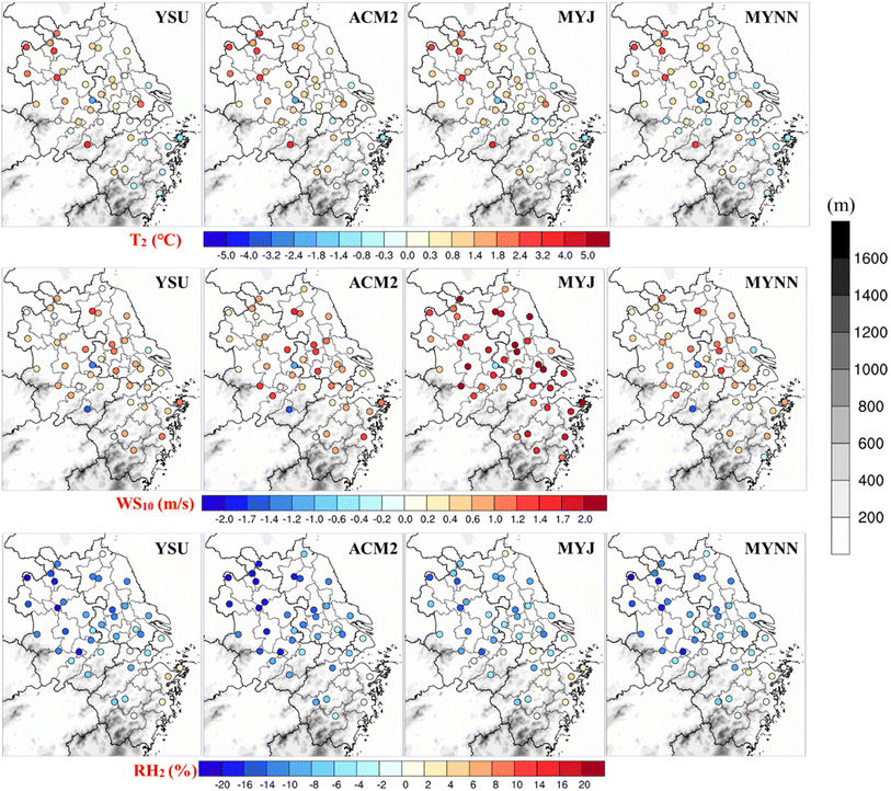
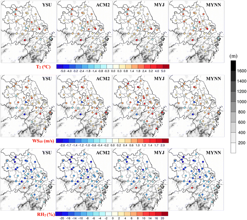
Table 2 summarizes the results of the statistical evaluation for the WRF-simulated meteorological variables, including T₂, WS₁₀, and RH₂, against the observations from 41 meteorological stations in the YRD region during July and November 2018. Furthermore, Fig. 2 provides a graphical representation of the comprehensive statistical evaluation metrics, i.e., MB, RMSE, NMB, NME and R, between the observed and simulated meteorological variables at the 41 stations. Additionally, time series plots of observed and simulated meteorological variables are presented in Fig. S1 and S2.†

Table 2 Statistics of model performance with different PBL schemes in July and November 2018

Indicators	July				November
	YSU	ACM2	MYJ	MYNN	YSU	ACM2	MYJ	MYNN
T 2 (°C)
MB (°C)	0.69	0.72	0.61	0.41	0.66	0.82	0.64	0.88
RMSE (°C)	2.71	2.62	2.63	2.50	2.28	2.31	2.26	2.34
NMB (%)	2.52	2.63	2.25	1.56	5.94	7.23	5.83	7.76
NME (%)	7.19	6.92	7.00	6.61	14.92	15.34	14.78	15.50
R	0.73	0.76	0.76	0.76	0.85	0.86	0.86	0.85
WS 10 (m s^− ^1 )
MB (m s^−1)	0.47	0.66	1.55	0.44	0.40	0.49	0.69	0.35
RMSE (m s^−1)	2.04	2.10	2.76	2.01	1.76	1.77	1.94	1.73
NMB (%)	17.83	24.26	52.29	17.18	20.23	24.41	32.34	18.15
NME (%)	50.71	53.56	70.87	51.17	56.52	57.67	62.57	55.79
R	0.47	0.47	0.46	0.46	0.47	0.48	0.51	0.46
RH 2 (%)
MB (%)	−8.57	−10.51	−5.81	−8.31	−9.34	−11.68	−5.76	−10.88
RMSE (%)	15.90	16.67	13.38	15.15	17.17	18.73	14.94	17.63
NMB (%)	−10.65	−13.07	−7.21	−10.30	−11.27	−14.11	−6.90	−13.13
NME (%)	15.50	16.43	13.11	14.80	16.24	18.02	13.99	17.02
R	0.62	0.64	0.68	0.65	0.64	0.62	0.66	0.66

---

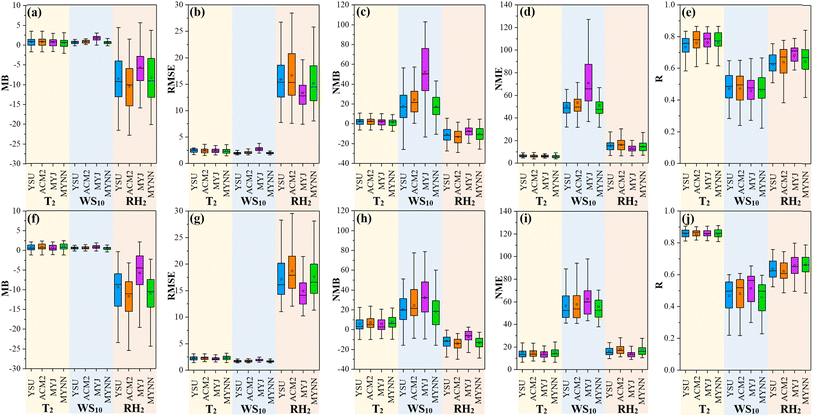Fig. 2 Statistical indicators for the evaluation in 41 cities of the YRD region in July (a–e) and November (f–j) 2018.

3.1.1 Temperature. Time series of the simulated T₂ for the 41 stations (mentioned previously) in July and November (Fig. S1a and S2a†) shows general consistency with observations, which is the common outcome from most temperature simulation studies.^64–69 As summarized in Table 2, all the four PBL schemes exhibit temperature overestimations in both summer and winter, among which MYNN and MYJ respectively show the least bias in summer and winter. In summer, MYNN performs the best with the lowest MB of 0.41 °C, a RMSE of 2.50 °C, a NMB of 1.56%, a NME of 6.61%, and a high value of R (0.76). In contrast, ACM2 shows the largest summer overestimation with an MB of 0.72 °C. For winter, MYJ stands out with the least values of MB (0.64 °C), NMB (5.83%), and NME (14.78%), and a strong value of R (0.86), while MYNN shows the largest overestimations with a MB of 0.88 °C. It is noteworthy that the limitations of utilizing NMB and NME for temperature modeling evaluation would exaggerate relative errors particularly in the winter with lower temperatures. Comparing the RMSE by using four schemes in two seasons, the temperature overestimations are more pronounced in summer relative to winter generally.

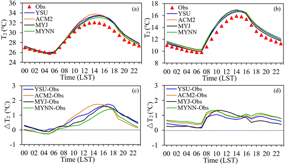
The average diurnal variations of T₂ simulated by using four PBL schemes are compared with the observations in Fig. 3, demonstrating the reasonable fluctuations throughout the day. Although daytime T₂ values in summer are generally higher, simulated values are slightly lower than observations early in the morning (Fig. 3c). In contrast, T₂ simulations consistently overestimate values during winter (Fig. 3d). Our findings align with those of Hariprasad et al.,⁴³ who found a warm bias in daytime temperature across most PBL schemes. Notably, significant discrepancies in T₂ simulation arise among the four schemes due to different treatments of physical processes within the boundary layer, even with similar land surface parameters.⁷⁰ ACM2 and YSU tend to yield higher temperature bias at noon in summer than in winter. Our analysis reveals that YSU and ACM2 produce higher temperature overestimations in daytime during summer, while MYNN produces the least deviation in temperature. This is likely attributed to enhanced vertical mixing in the lower PBL by MYNN, which will be analyzed further in Section 3.3. Furthermore, simulations of nighttime T₂ by the local closure MYJ scheme are better than those by the non-local closure schemes and another local closure MYNN during winter, suggesting that MYJ simulates stable stratification better in the night time. These variations in temperature simulations highlight the necessity for further investigation into the distinct physical processes simulated by each PBL scheme.

Fig. 3 Average diurnal variations of T₂ in summer (a) and winter (b); average diurnal differences (simulation minus observation) of T₂ in summer (c) and winter (d).

3.1.2 Wind speed. Table 2 shows that all four PBL schemes overestimate wind speed in the YRD region. This tendency toward overestimation has been also reported in other studies, such as those by Cheng and Steenburgh⁷¹ and Mölders.⁷² Among the four schemes, MYNN exhibits minimal overestimation of WS₁₀ in both summer and winter with the lowest MB of respectively 0.44 m s⁻¹ and 0.35 m s⁻¹. It is noteworthy that the R values for WS₁₀ by non-local closure schemes, i.e., YSU and ACM2, are slightly higher compared to those by local closure schemes in summer. However, MYJ produces the largest biases in terms of MB, RMSE, NMB, and NME in both summer and winter, although it shows the highest R of 0.51 in winter. Notably, another local closure scheme, MYNN, provides the lowest winter simulation bias of MB (0.35 m s⁻¹), RMSE (1.73), NMB (18.15%), and NME (55.79%). Moreover, the diurnal variations displayed in Fig. 4 indicate that YSU, ACM2, and MYNN schemes tend to overestimate WS₁₀ at nighttime, but their simulations during the daytime are almost in agreement with the observations. In contrast, MYJ exhibits the largest overestimations throughout the day, especially with the largest discrepancies identified during summer in the daytime, even up to 2 m s⁻¹. This overestimation might be explained by the lower shear stress simulated by MYJ due to its lower daytime friction velocity (shown in Section 3.4). Again, these findings underline the importance of exploring how various PBL schemes capture the physical processes influencing wind speed.

Fig. 4 Average diurnal variations of WS₁₀ in summer (a) and winter (b); average diurnal differences of WS₁₀ in summer (c) and winter (d).

3.1.3 Relative humidity. All four PBL schemes show an underestimation of RH₂, consistent with the findings of Misenis and Zhang,⁷³ who reported similar underestimations by the MYJ and YSU schemes in air quality simulations over coastal Mississippi. Coincidentally, Gunwani and Mohan⁷⁴ also reported a significant dry bias predicted by all PBL schemes in the temperate zone, compared to other climate zones. Note that the air capacity to hold water vapor increases exponentially as temperature increases, at a rate of about 6–7% per degree Celsius.⁷⁵ Thus, the atmosphere can hold more moisture at higher temperatures. It is necessary to consider the temperature bias for the evaluations of RH simulations. All the schemes show a dry bias in RH₂, which may be attributed to the overestimations of T₂. As shown in Table 2, the model overpredicts T₂ by a range of 0.41–0.88 °C, while underpredicting RH₂ by a range of −5.81–10.88%. This discrepancy possibly includes a dry bias of around −3.5% due to the overestimation of temperature. As depicted in Table 2 and Fig. 5, the MYJ scheme presents superior accuracy in predicting surface RH₂ in both summer and winter, exhibiting the lowest RMSE, MB, and NMB values and the highest R in both summer and winter. These are the closest diurnal differences to zero between the simulations of MYJ and observations. Besides, the ACM2 scheme produces the most significant dry bias in both seasons among the four schemes.

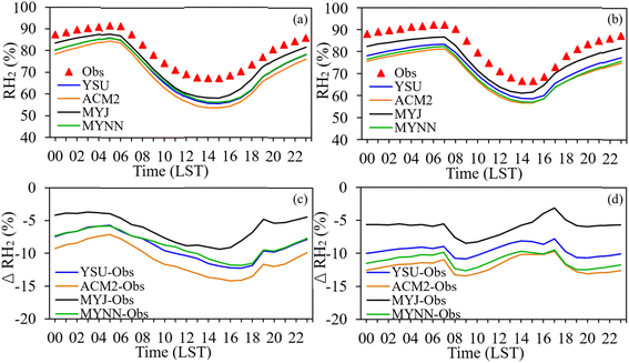Fig. 5 Average diurnal variations of RH₂ in summer (a) and winter (b); average diurnal differences of RH₂ in summer (c) and winter (d).

Fig. 5 reveals that all PBL schemes show significant underestimations of RH₂ during the daytime, with a notable reduction in the dry bias at night in summer. However, the dry bias at night becomes more evident during the winter compared to summer. The non-local closure schemes, YSU and ACM2, simulate a boundary layer with stronger mixing processes, resulting in tendencies to produce higher temperatures and lower relative humidity. On the other hand, the milder mixing of the MYJ scheme causes relatively higher simulated relative humidity compared to the other three PBL schemes, which will be further discussed in Section 3.3.

3.1.4 Spatial distribution of model biases. Fig. 6 and 7 show the spatial distributions of the MB of T₂, WS₁₀, and RH₂ in 41 cities within the YRD region in July and November, respectively. During summer, all PBL schemes exhibit an overestimation of T₂ over most of the northern plain areas in the YRD region, particularly in the northwestern areas, with the highest MB approaching 5.8 °C. However, T₂ in the southeast coastal areas is generally underestimated with the MB ranging between −0.6 °C and −0.2 °C. A similar result of slight underestimation can also be obtained in several northwestern cities in the YRD during winter. Thereinto, the MB of T₂ overestimation by ACM2 is statistically higher than that of the other three schemes, indicating that ACM2 tends to produce the highest simulated temperature among all schemes. In contrast to the temperature biases, RH₂ is predominantly underestimated over the YRD region, particularly in its northwestern regions. The simulated RH₂ in the southern and southeastern areas is closer to the observations than those in other areas in the YRD region. Among the four schemes, MYJ produces the lowest RH₂ bias in both summer and winter. Due to the relatively higher overestimation of temperature, ACM2 performs the most noticeable underestimation of RH₂. With respect to wind speed, MYJ produces the highest overestimation in most of the northern and middle plain areas of the YRD in both summer and winter, which demonstrates a more pronounced bias in the summer. In contrast, MYNN, followed by YSU and ACM2 schemes, exhibits the least bias for WS₁₀ in most of the areas of the YRD during both seasons, indicating its comparative reliability in wind speed simulations.

Fig. 6 Model bias (MB) of T₂, WS₁₀, and RH₂ in 41 cities of the YRD region in July 2018.

Fig. 7 Model bias of T₂, WS₁₀, and RH₂ in 41 cities of the YRD region in November 2018.

3.2 PBL height (PBLH)

One primary source of bias in mesoscale weather simulations is the choice of distinct simulation schemes to diagnose the PBLH. Different methods and parameters used in PBL formulations can lead to variable PBLHs. For instance, the YSU and ACM2 schemes determine PBLH when the bulk R_i exceeds a critical R_i of 0.25. Considering that a critical R_i of 0.25 is utilized in this study, the PBLH calculation relies on both the virtual potential temperature (θ_v) and wind shear.⁹ This could lead to more significant inaccuracies in the simulated wind speed, which corresponds with the observed overestimation of WS₁₀ for the YSU scheme. However, the MYJ and MYNN schemes diagnose PBLH based on a threshold TKE, identifying the PBLH when the first prognostic TKE reaches a sufficiently low value of around 0.005 m² s⁻².²⁵ To ensure consistency, this study applies the R_i-based method to determine the PBLH.

The results show that during summer, the mixing height is relatively deeper than in winter (Fig. 8). Similar findings were also reported by Kompalli et al.⁷⁶ over Nagpur. ACM2 produces deeper boundary layers in summer, followed by MYNN and YSU, with ACM2 showing the highest overestimation with a MB of 394 m and a maximum PBLH up to 2541 m. According to the statistics in Table 3, YSU reproduces more realistic diurnal variations of radiosonde data during summer, exhibiting the lowest bias and highest R followed by MYNN. Note that MYNN tends to produce a deeper mixing layer compared to YSU, ACM2, and MYJ in the morning in both summer and winter.

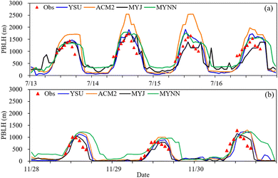Fig. 8 Diurnal variation of the PBL height simulated by different PBL schemes along with observations by using a radiosonde in summer (a) and winter (b).

Table 3 Comparison of the PBL height and model performance simulated by different PBL schemes

PBL scheme/season	PBL height (m)				Indicators
	Early morning (8LST)	Early afternoon (14LST)	Max	Min	MB (m)	R
Summer
YSU	437	1545	1911	101	102	0.81
ACM2	578	1952	2541	145	394	0.76
MYJ	550	1269	1690	147	−566	0.66
MYNN	605	1510	1795	111	172	0.79
Winter
YSU	116	920	1278	17	46	0.58
ACM2	140	1006	1301	30	75	0.60
MYJ	108	994	1142	20	38	0.65
MYNN	286	997	1236	47	48	0.49

---

Regarding winter simulations, the development of the boundary layer was slower than in summer, and all four schemes exhibited overestimations in the afternoon. MYJ demonstrates the most accurate performance for the PBLH in winter, exhibiting the least bias with an MB of 38 m and the highest correlation (R = 0.65). ACM2 and YSU produced relatively deeper boundary layers. The simulated PBL by ACM2 achieves maximum and minimum depths of 1301 m and 30 m, respectively. Subsequently, YSU simulated the PBLH ranging from 17 m to 1278 m. Such deep mixed layers calculated by ACM2 and YSU are consistent with those reported by Shin and Hong²⁵ for mid-latitudes and by Madala et al.²⁸ for Ranchi, respectively.

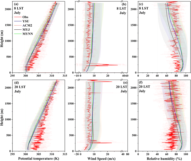
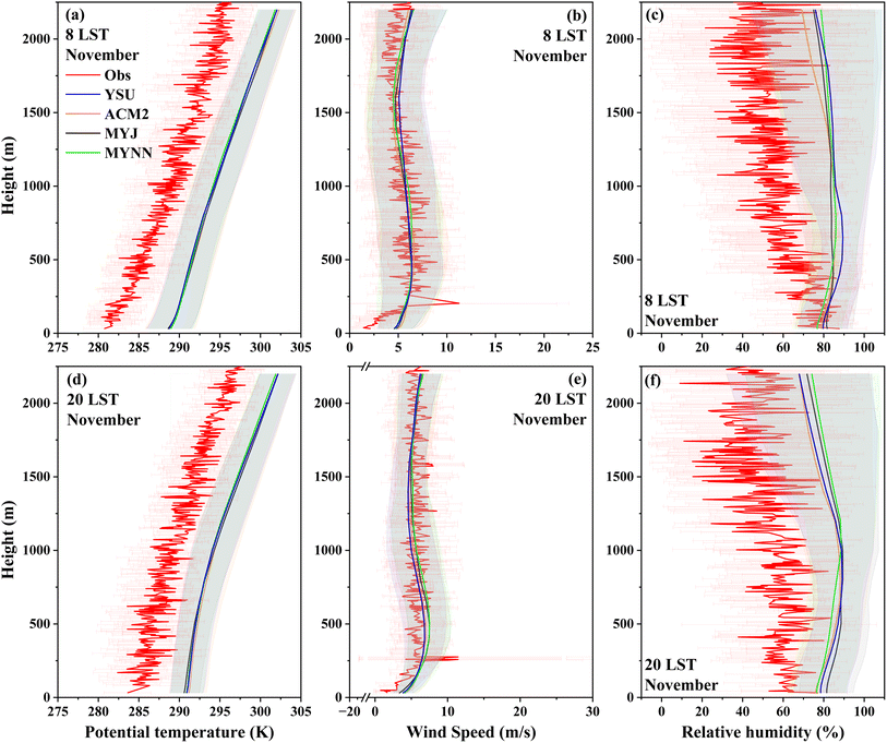
3.3 Thermodynamical structure of the atmosphere

The vertical distribution of meteorological parameters is a crucial indicator of the thermal and dynamic structure of the boundary layer. Fig. 9 and 10 illustrate the monthly average vertical profiles of potential temperature, wind speed, and relative humidity observed by using an L-band radiosonde at Fuyang (marked with a blue triangle in Fig. 1b) respectively at 08LST and 20LST in two seasons, as well as the corresponding simulated meteorological parameters. In summer, the observed and simulated potential temperature appears to have a consistent gradient with the simulated profiles generally following the observed trend within a close range both at 8 LST and 20 LST. However, simulated potential temperatures are relatively higher than the observations in winter. The simulations by four schemes generally tend to overestimate the wind speeds in summer but show some differences particularly at around 200 m. The simulated profiles attempt to capture the overall variations of wind speed in winter, while some discrepancies exist at lower altitudes in the morning. The simulations for the four schemes generally tend to overestimate the relative humidity in two seasons, while the simulations in summer at higher altitudes show lower relative humidity than the observations.

Fig. 9 Comparisons between simulated and observed monthly average vertical profiles of potential temperature (a and d), wind speed (b and e) and relative humidity (c and f) at 08LST and 20LST respectively in July.

Fig. 10 Comparisons of model simulated and observed monthly average vertical profiles of potential temperature (a and d), wind speed (b and e) and relative humidity (c and f) at 08LST and 20LST respectively in November.

Across all parameters, the observed data display more variability and smaller-scale fluctuations, while simulations offer smoothed representations capturing general trends. The simulated profiles generally follow the observed trends, and discrepancies are noted, particularly in capturing the finer details and variability of the observed data.

3.4 Turbulent fluxes and friction velocity

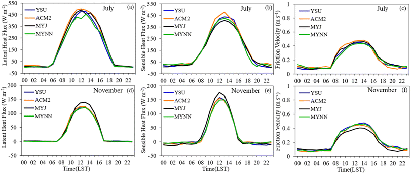
Surface fluxes such as sensible and latent heat flux play a crucial role in determining the characteristics of the boundary layer, as they serve as the forcing field at the lower boundary of the atmosphere.^77,78 In this study, we present the average diurnal variation of sensible heat, latent heat fluxes, and friction velocity simulated with different PBL schemes for July (Fig. 11a–c) and November (Fig. 11d–f). As the same land surface scheme is used in all simulations, the results obtained from different boundary layer schemes are similar.

Fig. 11 Time series of average simulated latent heat flux (a and d); sensible heat flux (b and e); and friction velocity (c and f). The panels above (a–c) are for July 2018 and panels below (d–f) are for November 2018.

Although the four PBL schemes exhibit similar diurnal variations of the surface heat fluxes, discrepancies exist in both latent and sensible heat flux during the daytime. Specifically, ACM2 produces a relatively larger simulation in two heat fluxes compared to other schemes in the summer daytime, while MYJ simulates a rather higher heat flux in the winter daytime. Overall, all simulations show higher latent and sensible heat fluxes during summer (∼450 W m⁻²) compared to that in winter (∼150 W m⁻²), consistent with previous findings by Hariprasad et al.⁴³

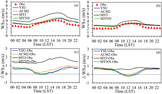
The simulation of friction velocity is critical for depicting the intensity of mechanical turbulence, which is helpful to clarify simulated surface-level winds. Additionally, different friction velocities simulated by each scheme can affect mixing lengths, resulting in discrepancies in wind speed simulations.^74,79,80 Comparing the diurnal variation of friction velocity, ACM2 produces higher daytime friction velocity than the other three schemes for summer, leading to a higher prediction of shear stress. This simulation has a significant impact on the strong mixing in the boundary layer during the daytime. Conversely, MYJ tends to simulate a lower daytime friction velocity rather than the other schemes. This lower friction velocity suggests a reduced momentum exchange between the surface and the atmosphere, potentially leading to an overestimation of near-surface wind speeds. This mechanism can help explain the highest wind bias modeled with the MYJ scheme, as detailed in Section 3.1, where we reported the largest overestimations during the summer daytime, reaching up to 2 m s⁻¹. By improving the understanding of this interaction, we can better address and refine the model to reduce such biases.

3.5 Limitations and uncertainties

While our study provides valuable insights into the proper selection of different PBL schemes for various meteorological modeling studies, it has several limitations. First, PBL closure schemes, such as MYJ and MYNN local closure schemes, may not accurately capture all physical processes, leading to performance variations, especially during transitional seasons and under specific diurnal conditions. Furthermore, the utilization of the critical Richardson number (R_i) should be carefully considered in future studies. Lastly, the observational data might be insufficient to capture long-term patterns and anomalies necessary for a more comprehensive evaluation of the PBL schemes.

In this work, we selected the year 2018 to represent an average meteorological year and focused on two seasons, summer and winter. However, these results may not be applicable to extreme weather conditions and transitional seasons like spring and autumn. Additionally, the rapid urbanization in the Yangtze River Delta (YRD) region has led to significant discrepancies in building distribution. Due to a lack of detailed data, we did not account for this factor, resulting in a certain high bias in the prediction of wind speed, as shown in Table 2.

4 Conclusions

This study assesses the impact of four commonly used PBL schemes (YSU, ACM2, MYJ, and MYNN) on simulated meteorological variables for air pollution modelling studies over the YRD region using the WRF mesoscale model, including the seasonal sensitivity analysis in summer and winter. The results demonstrate that despite certain consistencies in the simulated parameters among four PBL schemes, individual differences non-negligibly exist. A warm bias during the daytime period in summer is noted, as the MYNN scheme provides the best performance in estimating temperature in summer; in turn the MYJ scheme performs better in winter. Moreover, the MYNN scheme results in the least bias of wind speed during both summer and winter. For relative humidity, the MYJ scheme performs reasonably well in both seasons. Overall, the local closure MYNN and MYJ schemes outperform the non-local closure YSU and ACM2 schemes in simulating surface meteorological factors over the YRD region.

Based on our results, no single concrete PBL scheme can be identified universally for predicting the PBLH. However, some schemes perform notably better in specific seasons. When considering vertical profiles, ACM2 shows stronger turbulent mixing and entrainment compared to MYJ and MYNN. The profiles of ACM2 and YSU exhibit higher temperatures and mixed layers in summer, whereas MYJ produces shallower mixed layers over the YRD region and aligns closely with radiosonde observations during winter. Furthermore, modeling results show varying magnitudes of flows, mixed layer height, and surface heat fluxes. These drastic variations in the simulations can be attributed to the use of distinct formulations for simulating the relative roles of buoyancy and shear in controlling the entrainment flux by distinct PBL schemes. Overall, our analysis highlights the sensitivity of the simulations to the PBL scheme chosen in the model.

In conclusion, our study reveals significant differences among different PBL schemes, particularly in seasonal changes, which is critical for precise weather prediction. Moreover, detailed sensitivity analysis compares the performance of the PBL schemes in regional climate models, emphasizing that no single scheme universally excels in predicting the PBL height. Local closure schemes such as MYJ and MYNN generally produce more realistic simulations of meteorological parameters, with MYNN performing best in summer and MYJ showing better results under stable conditions during winter. YSU is found to have less bias in the PBLH during summer. However, it is important to note that each scheme has its strengths and weaknesses, and the selection of the most appropriate scheme should depend on the specific variables and scenarios being evaluated. Our study stands out by providing comprehensive performance metrics (including R and RMSE) for different PBL schemes in simulating meteorological conditions such as temperature, humidity, and wind speed. This work is particularly useful for users of the WRF model, as it offers clear guidance on selecting the most appropriate boundary layer scheme based on their specific research objectives and targets. For instance, users seeking more stable and continuous PBL simulations can opt for PBL schemes with higher R values, while those aiming for optimal simulation accuracy can choose schemes with superior RMSE results. This tailored approach ensures that researchers can achieve the best possible outcomes for their specific meteorological modeling needs.

Data availability

The model code and script are available at https://ruc.noaa.gov/wrf/wrf-chem/. Data are available upon request to the corresponding author.

Conflicts of interest

There are no conflicts to declare.

Acknowledgements

This study was financially supported by the National Natural Science Foundation of China (No. 42075144, 42375102, and 41875161), and the Shanghai International Science and Technology Cooperation Fund (No. 19230742500). We thank Prof. Xuhui Cai at Peking University for sharing the radio sounding data at Fuyang station.

References

1. W. Jia and X. Zhang, The role of the planetary boundary layer parameterization schemes on the meteorological and aerosol pollution simulations: A review, Atmos. Res., 2020, 239, 104890.
2. C. Draxl, A. N. Hahmann, A. Peña and G. Giebel, Evaluating winds and vertical wind shear from Weather Research and Forecasting model forecasts using seven planetary boundary layer schemes, Wind Energy, 2014, 17, 39–55.
3. M. García-Díez, J. Fernández, L. Fita and C. Yagüe, Seasonal dependence of WRF model biases and sensitivity to PBL schemes over Europe, Q. J. R. Meteorol. Soc., 2013, 139, 501–514.
4. X.-M. Hu, D. C. Doughty, K. J. Sanchez, E. Joseph and J. D. Fuentes, Ozone variability in the atmospheric boundary layer in Maryland and its implications for vertical transport model, Atmos. Environ., 2012, 46, 354–364.
5. G. Steeneveld, T. Mauritsen, E. De Bruijn, J. Vilà-Guerau de Arellano, G. Svensson and A. Holtslag, Evaluation of limited-area models for the representation of the diurnal cycle and contrasting nights in CASES-99, J. Appl. Meteorol. Climatol., 2008, 47, 869–887.
6. Z. Wang, A. Duan and G. Wu, Impacts of boundary layer parameterization schemes and air-sea coupling on WRF simulation of the East Asian summer monsoon, Sci. China: Earth Sci., 2014, 57, 1480–1493.
7. R. F. Banks and J. M. Baldasano, Impact of WRF model PBL schemes on air quality simulations over Catalonia, Spain, Sci. Total Environ., 2016, 572, 98–113.
8. F.-Y. Cheng, S.-C. Chin and T.-H. Liu, The role of boundary layer schemes in meteorological and air quality simulations of the Taiwan area, Atmos. Environ., 2012, 54, 714–727.
9. Y. Li, J. He, J. Li, H.-L. Ren, H. Wang, W. Luo, S. Gong, H. Che and X. Zhang, Sensitivity analysis of the WRF simulated planetary boundary layer height to synoptic conditions over eastern China, Atmos. Res., 2024, 303, 107330.
10. Y.-F. Ma, Y. Wang, T. Xian, G. Tian, C. Lu, X. Mao and L.-P. Wang, Impact of PBL schemes on multiscale WRF modeling over complex terrain, Part I: Mesoscale simulations, Atmos. Res., 2024, 297, 107117.
11. L. Shi, A. Zhu, L. Huang, E. Yaluk, Y. Gu, Y. Wang, S. Wang, A. Chan and L. Li, Impact of the planetary boundary layer on air quality simulations over the Yangtze River Delta region, China, Atmos. Environ., 2021, 263, 118685.
12. C. Wu, K. Luo, Q. Wang and J. Fan, Simulated potential wind power sensitivity to the planetary boundary layer parameterizations combined with various topography datasets in the weather research and forecasting model, Energy, 2022, 239, 122047.
13. H. A. Arregocés, R. Rojano and G. Restrepo, Sensitivity analysis of planetary boundary layer schemes using the WRF model in Northern Colombia during 2016 dry season, Dyn. Atmos. Oceans, 2021, 96, 101261.
14. M. C. Coniglio, J. Correia Jr, P. T. Marsh and F. Kong, Verification of convection-allowing WRF model forecasts of the planetary boundary layer using sounding observations, Weather Forecast., 2013, 28, 842–862.
15. S. G. Gopalakrishnan, F. Marks Jr, J. A. Zhang, X. Zhang, J.-W. Bao and V. Tallapragada, A study of the impacts of vertical diffusion on the structure and intensity of the tropical cyclones using the high-resolution HWRF system, J. Atmos. Sci., 2013, 70, 524–541.
16. M. Mohan and S. Bhati, Analysis of WRF model performance over subtropical region of Delhi, India, Adv. Meteorol., 2011, 621235.
17. R. K. Smith and G. L. Thomsen, Dependence of tropical-cyclone intensification on the boundary-layer representation in a numerical model, Q. J. R. Meteorol. Soc., 2010, 136, 1671–1685.
18. C. Yver, H. Graven, D. D. Lucas, P. Cameron-Smith, R. Keeling and R. Weiss, Evaluating transport in the WRF model along the California coast, Atmos. Chem. Phys., 2013, 13, 1837–1852.
19. D.-L. Zhang and W.-Z. Zheng, Diurnal cycles of surface winds and temperatures as simulated by five boundary layer parameterizations, J. Appl. Meteorol. Climatol., 2004, 43, 157–169.
20. J. Sanjay, Assessment of atmospheric boundary-layer processes represented in the numerical model MM5 for a clear sky day using LASPEX observations, Bound. Lay. Meteorol., 2008, 129, 159–177.
21. J. H. Kwun, Y.-K. Kim, J.-W. Seo, J. H. Jeong and S. H. You, Sensitivity of MM5 and WRF mesoscale model predictions of surface winds in a typhoon to planetary boundary layer parameterizations, Nat. Hazards, 2009, 51, 63–77.
22. B. Xie, J. C. Fung, A. Chan and A. Lau, Evaluation of nonlocal and local planetary boundary layer schemes in the WRF model, J. Geophys. Res.: Atmos., 2012, 117, D12103.
23. R. Kretschmer, C. Gerbig, U. Karstens and F.-T. Koch, Error characterization of CO₂ vertical mixing in the atmospheric transport model WRF-VPRM, Atmos. Chem. Phys., 2012, 12, 2441–2458.
24. L.-J. Que, W.-L. Que and J.-M. Feng, Intercomparison of different physics schemes in the WRF model over the Asian summer monsoon region, Atmos. Oceanic Sci. Lett., 2016, 9, 169–177.
25. H. H. Shin and S. Y. Hong, Intercomparison of planetary boundary-layer parametrizations in the WRF model for a single day from CASES-99, Bound. Lay. Meteorol., 2011, 139, 261–281.
26. Y. Chu, J. Li, C. Li, W. Tan, T. Su and J. Li, Seasonal and diurnal variability of planetary boundary layer height in Beijing: Intercomparison between MPL and WRF results, Atmos. Res., 2019, 227, 1–13.
27. J. Kala, J. Andrys, T. J. Lyons, I. J. Foster and B. J. Evans, Sensitivity of WRF to driving data and physics options on a seasonal time-scale for the southwest of Western Australia, Clim. Dynam., 2015, 44, 633–659.
28. S. Madala, A. Satyanarayana, C. Srinivas and M. Kumar, Mesoscale atmospheric flow-field simulations for air quality modeling over complex terrain region of Ranchi in eastern India using WRF, Atmos. Environ., 2015, 107, 315–328.
29. L. Li, J. An, L. Huang, R. Yan, C. Huang and G. Yarwood, Ozone source apportionment over the Yangtze River Delta region, China: Investigation of regional transport, sectoral contributions and seasonal differences, Atmos. Environ., 2019, 202, 269–280.
30. L. Li, J. An, M. Zhou, L. Qiao, S. Zhu, R. Yan, C. G. Ooi, H. Wang, C. Huang and L. Huang, An integrated source apportionment methodology and its application over the Yangtze River Delta region, China, Environ. Sci. Technol., 2018, 52, 14216–14227.
31. W. Choi and K. Y. Kim, Summertime variability of the western North Pacific subtropical high and its synoptic influences on the East Asian weather, Sci. Rep., 2019, 9, 7865.
32. Y. Huang, B. Wang, X. Li and H. Wang, Changes in the influence of the western Pacific subtropical high on Asian summer monsoon rainfall in the late 1990s, Clim. Dynam., 2018, 51, 443–455.
33. Y.-L. Lin, R. D. Farley and H. D. Orville, Bulk parameterization of the snow field in a cloud model, J. Appl. Meteorol. Climatol., 1983, 22, 1065–1092.
34. F. Chen and J. Dudhia, Coupling an advanced land surface–hydrology model with the Penn State–NCAR MM5 modeling system. Part I: Model implementation and sensitivity, Mon. Weather Rev., 2001, 129, 569–585.
35. J. S. Kain and J. M. Fritsch, Convective parameterization for mesoscale models: The Kain-Fritsch scheme, In The representation of cumulus convection in numerical models, ed. K. A. Emanuel and D. J. Raymond, Springer, 1993, pp. 165–170.
36. E. J. Mlawer, S. J. Taubman, P. D. Brown, M. J. Iacono and S. A. Clough, Radiative transfer for inhomogeneous atmospheres: RRTM, a validated correlated-k model for the longwave, J. Geophys. Res.: Atmos., 1997, 102, 16663–16682.
37. L. Li, A. Zhu, L. Huang, Q. Wang, Y. Chen, M. C. G. Ooi, M. Wang, Y. Wang and A. Chan, Modeling the impacts of land use/land cover change on meteorology and air quality during 2000-2018 in the Yangtze River Delta region, China, Sci. Total Environ., 2022, 829, 154669.
38. J. Ma and R. Zhang, Opposite interdecadal variations of wintertime haze occurrence over North China Plain and Yangtze River Delta regions in 1980–2013, Sci. Total Environ., 2020, 732, 139240.
39. S. Niu, R. Chen, Y. Zou, L. Dong, R. Hai and Y. Huang, Spatial distribution and profile of atmospheric short-chain chlorinated paraffins in the Yangtze River Delta, Environ. Pollut., 2020, 259, 113958.
40. L. Ming, L. Jin, J. Li, P. Fu, W. Yang, D. Liu, G. Zhang, Z. Wang and X. Li, PM_2.5 in the Yangtze River Delta, China: Chemical compositions, seasonal variations, and regional pollution events, Environ. Pollut., 2017, 223, 200–212.
41. Y. Yang, M. Zhang, Q. Li, B. Chen, Z. Gao, G. Ning, C. Liu, Y. Li and M. Luo, Modulations of surface thermal environment and agricultural activity on intraseasonal variations of summer diurnal temperature range in the Yangtze River Delta of China, Sci. Total Environ., 2020, 736, 139445.
42. J. Hu, Y. Li, T. Zhao, J. Liu, X.-M. Hu, D. Liu, Y. Jiang, J. Xu and L. Chang, An important mechanism of regional O₃ transport for summer smog over the Yangtze River Delta in eastern China, Atmos. Chem. Phys., 2018, 18, 16239–16251.
43. K. Hariprasad, C. V. Srinivas, A. B. Singh, S. V. B. Rao, R. Baskaran and B. Venkatraman, Numerical simulation and intercomparison of boundary layer structure with different PBL schemes in WRF using experimental observations at a tropical site, Atmos. Res., 2014, 145, 27–44.
44. A. E. Cohen, S. M. Cavallo, M. C. Coniglio and H. E. Brooks, A review of planetary boundary layer parameterization schemes and their sensitivity in simulating southeastern US cold season severe weather environments, Weather forecast., 2015, 30, 591–612.
45. A. J. Clark, M. C. Coniglio, B. E. Coffer, G. Thompson, M. Xue and F. Kong, Sensitivity of 24-h forecast dryline position and structure to boundary layer parameterizations in convection-allowing WRF Model simulations, Weather Forecast., 2015, 30, 613–638.
46. A. J. Deppe, W. A. Gallus Jr and E. S. Takle, A WRF ensemble for improved wind speed forecasts at turbine height, Weather Forecast., 2013, 28, 212–228.
47. J. C. F. Lo, Z. L. Yang and R. A. Pielke Sr, Assessment of three dynamical climate downscaling methods using the Weather Research and Forecasting (WRF) model, J. Geophys. Res.: Atmos., 2008, 113, D09112.
48. C. Steele, S. Dorling, R. Von Glasow and J. Bacon, Idealized WRF model sensitivity simulations of sea breeze types and their effects on offshore windfields, Atmos. Chem. Phys., 2013, 13, 443.
49. L. Su and J. C. Fung, Sensitivities of WRF-Chem to dust emission schemes and land surface properties in simulating dust cycles during springtime over East Asia, J. Geophys. Res.: Atmos., 2015, 120, 11215–11230.
50. A. Yerramilli, V. S. Challa, V. B. Rao Dodla, H. P. Dasari, J. H. Young, C. Patrick, J. M. Baham, R. L. Hughes, M. G. Hardy and S. J. Swanier, Simulation of surface ozone pollution in the central gulf coast region using WRF/Chem Model: Sensitivity to PBL and Land Surface Physics, Adv. Meteorol., 2010, 319138.
51. J. Pleim, A combined local and nonlocal closure model for the atmospheric boundary layer. Part I: Model description and testing, J. Appl. Meteorol. Climatol., 2007, 46, 1383–1395.
52. M. Huang, Z. Gao, S. Miao and F. Chen, Sensitivity of urban boundary layer simulation to urban canopy models and PBL schemes in Beijing, Meteorol. Atmos. Phys., 2019, 131, 1235–1248.
53. Z. I. Janjić, The step-mountain coordinate: Physical package, Mon. Weather Rev., 1990, 118, 1429–1443.
54. X.-M. Hu, J. W. Nielsen-Gammon and F. Zhang, Evaluation of three planetary boundary layer schemes in the WRF model, J. Appl. Meteorol. Climatol., 2010, 49, 1831–1844.
55. M. Nakanishi and H. Niino, An improved Mellor–Yamada level-3 model: Its numerical stability and application to a regional prediction of advection fog, Bound. Lay. Meteorol., 2006, 119, 397–407.
56. N. Chaouch, M. Temimi, M. Weston and H. Ghedira, Sensitivity of the meteorological model WRF-ARW to planetary boundary layer schemes during fog conditions in a coastal arid region, Atmos. Res., 2017, 187, 106–127.
57. P. Li, G. Fu, C. Lu, D. Fu and S. Wang, The formation mechanism of a spring sea fog event over the Yellow Sea associated with a low-level jet, Weather Forecast., 2012, 27, 1538–1553.
58. C. Román-Cascón, C. Yagüe, M. Sastre, G. Maqueda, F. Salamanca and S. Viana, Observations and WRF simulations of fog events at the Spanish Northern Plateau, Adv. Sci. Res., 2012, 8, 11–18.
59. D. J. Seidel, Y. Zhang, A. Beljaars, J. C. Golaz, A. R. Jacobson and B. Medeiros, Climatology of the planetary boundary layer over the continental United States and Europe, J. Geophys. Res.: Atmos., 2012, 117, D17106.
60. S. Zhang, Z. Ren, J. Liu, Y. Yang and X. Wang, Variations in the lower level of the PBL associated with the Yellow Sea fog-new observations by L-band radar, J. Ocean Univ. China, 2008, 7, 353–361.
61. E. McGrath-Spangler and A. Molod, Comparison of GEOS-5 AGCM planetary boundary layer depths computed with various definitions, Atmos. Chem. Phys., 2014, 14, 6717–6727.
62. Y. Zhang, D. J. Seidel and S. Zhang, Trends in planetary boundary layer height over Europe, J. Clim., 2013, 26, 10071–10076.
63. R. Davy, The climatology of the atmospheric boundary layer in contemporary global climate models, J. Clim., 2018, 31, 9151–9173.
64. T. M. Giannaros, D. Melas, I. A. Daglis, I. Keramitsoglou and K. Kourtidis, Numerical study of the urban heat island over Athens (Greece) with the WRF model, Atmos. Environ., 2013, 73, 103–111.
65. C. Hogrefe, G. Pouliot, D. Wong, A. Torian, S. Roselle, J. Pleim and R. Mathur, Annual application and evaluation of the online coupled WRF–CMAQ system over North America under AQMEII phase 2, Atmos. Environ., 2015, 115, 683–694.
66. T. Li, H. Wang, T. Zhao, M. Xue, Y. Wang, H. Che and C. Jiang, The impacts of different PBL schemes on the simulation of PM_2.5 during severe haze episodes in the Jing-Jin-Ji region and its surroundings in China, Adv. Meteorol., 2016, 6295878.
67. M. S. Mallard, C. G. Nolte, O. R. Bullock, T. L. Spero and J. Gula, Using a coupled lake model with WRF for dynamical downscaling, J. Geophys. Res.: Atmos., 2014, 119, 7193–7208.
68. M. O. Mughal, X. X. Li, T. Yin, A. Martilli, O. Brousse, M. A. Dissegna and L. K. Norford, High-Resolution, Multilayer Modeling of Singapore's Urban Climate Incorporating Local Climate Zones, J. Geophys. Res.: Atmos., 2019, 124, 7764–7785.
69. Y. Wang, S. Di Sabatino, A. Martilli, Y. Li, M. Wong, E. Gutiérrez and P. Chan, Impact of land surface heterogeneity on urban heat island circulation and sea-land breeze circulation in Hong Kong, J. Geophys. Res.: Atmos., 2017, 122, 4332–4352.
70. S.-M. Lee, W. Giori, M. Princevac and H. Fernando, Implementation of a stable PBL turbulence parameterization for the mesoscale model MM5: nocturnal flow in complex terrain, Bound. Lay. Meteorol., 2006, 119, 109–134.
71. W. Y. Cheng and W. J. Steenburgh, Evaluation of surface sensible weather forecasts by the WRF and the Eta models over the western United States, Weather Forecast., 2005, 20, 812–821.
72. N. Mölders, Suitability of the Weather Research and Forecasting (WRF) model to predict the June 2005 fire weather for Interior Alaska, Weather Forecast., 2008, 23, 953–973.
73. C. Misenis and Y. Zhang, An examination of sensitivity of WRF/Chem predictions to physical parameterizations, horizontal grid spacing, and nesting options, Atmos. Res., 2010, 97, 315–334.
74. P. Gunwani and M. Mohan, Sensitivity of WRF model estimates to various PBL parameterizations in different climatic zones over India, Atmos. Res., 2017, 194, 43–65.
75. X. Gao, Q. Zhu, Z. Yang, J. Liu, H. Wang, W. Shao and G. Huang, Temperature Dependence of Hourly, Daily, and Event-based Precipitation Extremes Over China, Sci. Rep., 2018, 8, 17564.
76. S. K. Kompalli, S. S. Babu, K. K. Moorthy, M. Manoj, N. K. Kumar, K. H. B. Shaeb and A. K. Joshi, Aerosol black carbon characteristics over Central India: Temporal variation and its dependence on mixed layer height, Atmos. Res., 2014, 147, 27–37.
77. J. Panda and M. Sharan, Influence of land-surface and turbulent parameterization schemes on regional-scale boundary layer characteristics over northern India, Atmos. Res., 2012, 112, 89–111.
78. J. Rajeswari, C. Srinivas, T. N. Rao and B. Venkatraman, Impact of land surface physics on the simulation of boundary layer characteristics at a tropical coastal station, Atmos. Res., 2020, 238, 104888.
79. M. A. Kleczek, G.-J. Steeneveld and A. A. Holtslag, Evaluation of the weather research and forecasting mesoscale model for GABLS3: impact of boundary-layer schemes, boundary conditions and spin-up, Bound. Lay. Meteorol., 2014, 152, 213–243.
80. C. Onwukwe and P. L. Jackson, Meteorological downscaling with WRF model, version 4.0, and comparative evaluation of planetary boundary layer schemes over a complex coastal airshed, J. Appl. Meteorol. Climatol., 2020, 59, 1295–1319.

---

Footnotes

† Electronic supplementary information (ESI) available. See DOI: https://doi.org/10.1039/d4ea00038b

‡ These authors contributed equally to this work.

---