Simultaneous ionic cobalt sensing and toxic Congo red dye removal: a circular economic approach involving silver-enhanced fluorescence

Abstract

A highly fluorescent quinone-capped silver hydrosol (AgOSA) was obtained using salicylaldehyde and an ionic silver solution. Such metal-enhanced fluorescence was efficiently quenched with Congo red dye (CR), producing CRAgOSA, due to the strong silver–sulfur interaction, replacing the capping of quinone (oxidized salicylaldehyde). The introduction of cobalt ions restored the fluorescence by engaging CR (CoCRAgOSA). Cobalt-induced fluorescence enhancement was 8.3 times higher than that of AgOSA due to the freeing of CR and the release of self-quenching of excess quinone molecules in CoCRAgOSA. The mammoth and selective fluorescence enhancement with ionic cobalt assisted in designing a turn-on ionic cobalt sensor with a limit of detection (LOD) of 9.4 × 10⁻¹¹ M and a linear detection range (5 × 10⁻⁵ to 10⁻⁹ M). Moreover, toxic CR dye was eliminated by quinone-capped silver nanoparticles and Co²⁺ due to chemisorption. Not only the fluorimetric sensing of ionic cobalt but also the colorimetric sensing of Hg²⁺ was designed due to the simultaneous aggregation of AgNPs and complexation with CR induced by Hg²⁺ (LOD 1.36 × 10⁻⁵ M and linear detection range from 1.00 × 10⁻⁴ to 5 × 10⁻⁷ M). We applied our sensing method to estimate ionic cobalt and mercury in natural samples. The experiment was a unique case of circular economy, where a toxic dye was used for making a nanosensor.

---

1. Introduction

Several structures utilizing metals from the macroscopic down to the nanoscopic surface have been designed to change fluorescence signals (enhancement, quenching) to near-optical fields. Proximal fluorophores—those with lengths between 5 and 90 nm—interact favorably with a metallic surface, producing advantageous optical properties, including increased photostability, reduced lifetime, and increased quantum yield. This phenomenon, known as metal-enhanced fluorescence or MEF, has found extensive use in medicinal science.^1–3

The coinage metals in group 11, specifically copper (Cu), silver (Ag), and gold (Au), have greatly attracted the attention of scientists investigating the extensive group of transition metals.⁴ Silver nanostructures have garnered significant interest due to their exceptional plasmonic properties. The dielectric function of silver exhibits a minimal imaginary component across a wide range of wavelengths, and its real component is notably more negative compared to gold. The attributes of silver nanostructures (AgNPs) make them very suitable for sensing applications that rely on the localized surface plasmon resonance (LSPR) phenomena.⁵

Human health suffers when water is contaminated with various substances, such as harmful heavy metals and dyes.⁶ The elements that make up the heavy metal group are heterogeneous, with differences in their chemical makeup and roles. The transition element in the periodic table is mostly where heavy metals are found. Elements with a specific weight greater than 5 g cm⁻³ are classified as heavy metals. Moreover, those that have a density of at least five times that of water are classified as heavy metals.^7–11

Cobalt has positive effects on human health (in some metabolic and biological processes), but when the levels of cobalt reach permissible limits, it can have negative effects on the body. This emphasizes how crucial it is to create rapid detection methods with detection time of a few seconds, sufficient precision (low limit of detection) and ability to process small sample volumes for cobalt detection.^5,12,13

Long-term exposure to even low quantities of mercury may seriously harm a variety of organs since it is a very poisonous element. The maximum contamination limit for mercury, as determined by the US Environmental Protection Agency (EPA), is just 10 ng.¹⁴ The WHO has classified mercury as one of the top 10 substances or groups of compounds of serious public health concern. Mercury is known to have an accumulative nature and is extensively dispersed in the air, water, and soil. Because of its high water solubility, the solvated divalent mercuric ion (Hg²⁺), the most stable form of inorganic mercury, is mostly found in aquatic habitats. People of all ages may suffer harm to their brain, heart, kidneys, lungs, and immune systems from high concentrations of Hg²⁺ exposure.^15,16

A major family of synthetic colorants, azo dyes like Congo Red (CR), is utilized in textile manufacturing because of their energy-saving qualities, resistance to decolorization, and wide shade range.¹⁷ The azo dyes may contain aromatic rings and one or more chromophoric groups. Because of their resonance and π-conjugated azo bond properties, azo dyes are highly robust in light and harsh conditions. For this reason, they are suggested for use in the chemical, paper, cosmetic, and pharmaceutical sectors, among other industries.^6,18,19

Up to 108 tonnes of various dyes are generated each year around the world; azo dyes account for 60–70% of the total. The widespread use of azo dyes results in a high concentration of azo dye contaminants in wastewater. Because the diazo dye, also known as Congo Red, has an aromatic amine in its composition, it is known to be carcinogenic. The resistance of azo dyes to natural degradation is attributed to their aromatic nature. Long-term environmental exposure to dyes has detrimental impacts on both plant and animal life.²⁰

As a result, treating water contaminated with CR dyes is essential. A variety of techniques, including adsorption, coagulation–flocculation, ultrasonic irradiation, ion exchange, mineralization, and photocatalysis, have been proposed to remove CR from contaminated water. Among them, adsorption has a long history²¹ and is likely to remain popular because of its many benefits, including low cost, plenty of readily accessible adsorbents, high adsorption capacity, simple regeneration potential, and low energy consumption. The adsorption process is influenced by the kind and characteristics of the adsorbent. More investigation into the application of different adsorbents for the removal of CR dye from wastewater has been realized.⁶

This research revealed a silver hydrosol (AgOSA) with significant MEF. AgOSA was utilized mainly for fluorometric cobalt ion detection when CR was adsorbed on the AgOSA + Co²⁺ system. Furthermore, Hg²⁺ was also detected by the naked eye and colorimetrically due to the remarkable color change of CRAgOSA (CR + AgOSA) from red to blue.

For the first time, MEF was used to remove the toxic Congo red dye and to sense Co²⁺ and Hg²⁺ in one pot. The elimination of a toxic dye was associated with chemosensing, implying a circular economical approach. Previously, we reported silver-enhanced fluorescence for sensing applications.²² However, in the present study, the presence of a toxic dye caused the quenching of MEF, which originated from Ag⁰ and OSA. Co²⁺ turned on the fluorescence selectively and sensitively. Hg²⁺ remarkably changed the color of the dye-treated silver hydrosol. This is a unique research study on simultaneous environmental remediation and nanosensing.

2. Experimental section

All of the compounds used in the research were of analytical grade without the need for further purification. Triple-distilled water was used for the whole undertaking. After preparing the new aqua regia, soapy water and large amounts of distilled water were used to clean all the glassware. The glassware were completely dried before use. Silver nitrate was purchased from Sigma-Aldrich. Fisher Scientific and Qualigens supplied the NaOH. Loba Chemicals was the supplier of salicylaldehyde (SA) and all of the metal salts. A digital spectrophotometer was used to record the UV/Vis absorption spectra (Shimadzu UV-2600). At room temperature, the fluorescence was examined using a Horiba FluoroMax-4 spectrophotometer. Particle morphology was examined using a JEOL JSM-7610FPlus FESEM instrument, a high-resolution (1 kV 1.0 nm, 15 kV 0.8 nm) scanning electron microscope with a broad variety of probes. Samples were vacuum-dried for twenty-four hours before the FESEM experiment. The aqueous suspension was dried on carbon tape for microscopic inspection. Using an X-ray diffractometer (model: SMARTLAB), X-ray diffraction (XRD) patterns were recorded.

A VG Scientific ESCALAB MK II spectrometer (UK) fitted with a five-channeltron detection system and a Mg Kα excitation source (1253.6 eV) was used for obtaining the X-ray photoelectron spectra (XPS).

2.1 Synthesis of AgOSA

SA (0.015 M) in NaOH (10⁻² M) and AgNO₃ (10⁻³ M) were added to produce the yellowish-green fluorescent hydrosol AgOSA after ∼2 h of aging under sunlight.

3. Results and discussion

3.1 AgOSA: quinone-capped emissive silver hydrosol

A highly emissive silver hydrosol (AgOSA) was synthesized by aging alkaline SA with silver nitrate solution for 2 h under sunlight. SA remained in the phenolate form in an alkaline solution. SA reduced Ag⁺ to Ag⁰, while SA was oxidized to quinone form (OSA). OSA stabilized the Ag⁰ nanoparticles in AgOSA. We monitored the fluorescence of AgOSA at each 24 h interval for one week, keeping the hydrosol at room temperature on the bench. No significant change in the fluorescence intensity and wavelength was observed after a week of aging. Fig. 1 shows the emission (λ_em = 419 nm), absorption (λ_max = 232 nm, 296 nm, and 396 nm), and excitation spectra (λ_ex = 320 nm) of AgOSA. We varied various excitation energies to record the fluorescence and 320 nm was found to be the optimum excitation energy to obtain the highest fluorescence intensity (Fig. S1, ESI†). A lattice fringe of 0.237 nm corroborated to Ag⁰ particles for the (111) crystal plane.²³ The binding energies of 368.9 and 374.9 eV, obtained from the XPS spectra, corresponded to the 3d_5/2 and 3d_3/2 states for zero-valent silver, respectively.²⁴ Silver and other elements were also assigned in the XPS full spectrum (Fig. S2, ESI†). The binding energy of 367.6 eV corresponds to the 3d_5/2 state for Ag⁺. We did not find evidence of the presence of Ag⁺ in AgOSA from the XPS analysis (Fig. 2).²⁵

Fig. 1 (a) Emission; (b) absorption and (c) excitation spectra of AgOSA.

Fig. 2 (a) HRTEM image and (b) XPS spectra of AgOSA.

From the XRD pattern, it is evident that silver was in the zero oxidation state (2θ values of 38°, 44°, 64°, and 77° represent (111), (200), (220), and (311), respectively).²⁶ DLS analysis indicated the hydrodynamic radius of the particles in AgOSA to be 97.36 nm. The hydrosol was highly stable for greater than a week without any significant change in the fluorescence intensity. The capping agent OSA exerted a negative charge on the particle surface with a zeta potential of −36 ± 1.6 mV, the driving force of the stability. The SEM image indicated aggregated particles of AgNPs, thus leading to MEF. The radiating plasmon model, illustrated by Lakowicz,²⁷ showed larger fluorescence enhancements with particle aggregates displaying longer wavelength extinction (Fig. 3). A higher rate of excitation of the fluorophore in the presence of a metalized silver surface (lightening rod effect) was attributed to MEF.^28,29

Fig. 3 (a) XRD pattern, (b) DLS spectra, (c) zeta potential, and (d) SEM image of AgOSA.

3.2 Fluorimetric sensing of Co²⁺

Thus, the Ag⁰ nanoparticles increased the fluorescence intensity of weakly fluorescent OSA due to a higher rate of excitation in the presence of a metal surface. The strong fluorescence of AgOSA was quenched drastically in the presence of CR (CRAgOSA). CR is a sulfur-containing dye with a fused aromatic ring.³⁰ The sulfur group has a strong affinity towards silver.³¹ Thus, Ag–S interaction caused trapped surface plasmons and converted radiative energy to non-radiative energy, resulting in fluorescence quenching. In CRAgOSA, different metal ions (Cu⁺, Al³⁺, Zn²⁺, Ca²⁺, Co²⁺, Mg²⁺, Cr³⁺, Fe³⁺, Hg²⁺, Ni²⁺, Na⁺, K⁺ and Pb²⁺) were added. Surprisingly, Co²⁺ enhanced the fluorescence selectively (CoCRAgOSA). No other metal ion could enhance the fluorescence of CRAgOSA. With the increase in [Co²⁺], the fluorescence of CRAgOSA was gradually increased. Thus, a Co²⁺ sensor was designed with a limit of detection of 9.4 × 10⁻¹¹ M and a linear detection range from 5 × 10⁻⁵ to 10⁻⁹ M (Fig. 4).

Fig. 4 (a) Fluorescence spectra of CRAgOSA in the presence of various metal ions; (b) bar diagram of I/I₀ for different metal ions; (c) fluorescence spectra of CRAgOSA with different [Co²⁺]; (d) plot of I/I₀vs. [Co²⁺] and linear detection range of Co²⁺ detection.

In the highly fluorescent CoCRAgOSA, other interfering metal ions (Ca²⁺, Ba²⁺, Cr³⁺, Al³⁺, Mg²⁺, Hg²⁺, Fe³⁺, Cu²⁺, Na⁺, K⁺, Zn²⁺, and Pb²⁺) were added to gauge the effect of coexisting metal ions. However, no drastic change was observed in the fluorescence intensity of CoCRAgOSA except for Fe³⁺ (Fig. S3, ESI†). Fe³⁺ makes a complex with SA, hindering the capping of AgNPs. Reddish-orange complexes were created by Jain and Kumar³² using iron(III) and salicylaldehyde hydrazone in an alkaline pH range of pH 10–11. A stable ferrous complex was finally formed from the unstable Fe(III)-salicylaldehyde combination. There are only a few reports available for cobalt-ion sensing. Our proposed method not only enriched the fundamental understanding but also showed better LOD, detection range, and ease of use (Table 1).

Table 1 Detection of Co²⁺ with AgNPs by different research groups

AgNPs	Method of detection	LOD of Co^2+	Range of detection
Tyrosine capped AgNPs^12	Fluorescent sensor	48 ppb	0.1–9 μM
Dopamine dithiocarbamate^13	Colorimetric sensor	14 μM	1.0–15 mM
Povidone-capped AgNPs^33	Colorimetric sensor	0.1 μM	0.1–10 μM
L-Cysteine-functionalized Ag–Ag nanotriangles^5	Based on surface plasmon resonance	3.5 nM	10–100 nM
3-Mercapto-1-propanesulfonic acid sodium salt-capped AgNPs^34	Plasmonic sensor	500 ppb	0.5–2.0 ppm
Triazole-carboxyl AgNPs^35	Colorimetric sensor	7.0 × 10^−6 M	5.0 × 10^−6 to 1.0 × 10^−4 M
Homocysteine and rhodamine 6G derivatives-functionalized AgNPs^36	Fluorescent sensor	0.037 μM	0.10–25 μM
Our present method	Fluorescent sensor	9.4 × 10^− ^11 M	10^− ^5 –10^− ^9 M

---

3.3 Estimation of Co²⁺ in the natural sample

Co²⁺ was estimated using our mentioned fluorometric protocol not only in distilled water (used in the laboratory) but also in natural water samples [Ganga water (Haridwar) rainwater (Jaipur), drinking water (Jaipur), tap water (Jaipur), and water from melted ice (Shimla)]. We added varying quantities of Co²⁺ to the real water samples. The closeness to the actual spiking concentrations was achieved via the obtained fluorometric data (Table 2).

Table 2 Estimation of Co²⁺ in various natural water samples

Sample name	Added [Co^2+] (M)	[Co^2+] detected (M)	Recovery (%)	Relative error (%)	RSD (%) (n = 3)
Ganga water (Haridwar)	5.00 × 10^−5	5.20 × 10^−5	104	4	1.4
	5.00 × 10^−4	4.94 × 10^−4	98.8	1.2	2.1
	5.00 × 10^−3	5.20 × 10^−3	104	4	0.3
Rainwater (Jaipur)	5.00 × 10^−5	4.84 × 10^−5	98.8	1.2	0.3
	5.00 × 10^−4	5.10 × 10^−4	102	2	2.2
	5.00 × 10^−3	5.11 × 10^−3	102.2	2.2	2.1
Drinking water (Jaipur)	5.00 × 10^−5	4.89 × 10^−5	97.8	2.2	0.8
	5.00 × 10^−4	4.99 × 10^−4	99.8	0.2	2.6
	5.00 × 10^−3	4.89 × 10^−3	97.8	2.2	1.0
Tap water (Jaipur)	5.00 × 10^−5	5.12 × 10^−5	102.2	2.2	1.1
	5.00 × 10^−4	5.18 × 10^−4	103.6	3.6	0.5
	5.00 × 10^−3	4.94 × 10^−3	98.8	1.2	0.5
Water from melted ice (Shimla)	5.00 × 10^−5	4.95 × 10^−5	99	1	2.7
	5.00 × 10^−4	5.08 × 10^−4	101.6	1.6	3.0
	5.00 × 10^−3	5.08 × 10^−3	101.6	1.6	1.4

---

3.4 Mechanism of Co²⁺ sensing

The fluorescence enhancement of CoCRAgOSA was not just due to the restoration of fluorescence of AgOSA. The fluorescence enhancement was 8.3 times higher than that of AgOSA. Co²⁺ removed CR from the proximity of AgNPs, rendering the silver surface free to MEF. The CR dye underwent metal functionalization with cobalt, resulting in CR as a ligand. The metal–ligand interaction between CR and cobalt complexes can produce new functional materials, as illustrated by Setyawati et al.³⁷

Furthermore, Co²⁺ removed the self-quenching of the fluorophore, bestowing more MEF than that of AgOSA. Increasing the number of fluorophores using high-density labeling is an easy way to raise the signal-to-noise ratio and, thus, the detection limit. Higher concentrations of the fluorophore solution decreased the intensity of fluorescence emission, causing self-quenching. Numerous processes, including collisions between excited fluorophores, formation of non-fluorescent dimers, and energy transfer to the non-fluorescent dimers, can lead to self-quenching.³⁸ There is no report of direct complex formation available in the literature regarding SA and cobalt. However, the strong affinity of SA with cobalt was illustrated by Xu et al.³⁹ They synthesized a Schiff base-derived from SA (salicylaldehyde 2-phenylquinoline-4-carboylhydrazone) with strong complexation with Co²⁺. Nishikawa and Yamada prepared planar quadri-co-ordinate complexes of cobalt(II) with Schiff Bases (derived from SA).⁴⁰ Co²⁺ removed excess (uncapped) SA/OSA from the hydrosol-forming CoSA complex in the present case, releasing the self-quenching (Scheme 1).

Scheme 1 Mechanistic representation of cobalt-induced restoration of fluorescence.

The precipitate obtained from CoCRAgOSA hydrosol was washed thoroughly and the XRD pattern was recorded. Fig. 5 indicates the presence of only zero-valent silver at 2θ values of 38°, 44°, 64°, and 77°, representing the planes (111), (200), (220), and (311), respectively, when silver is in the zero oxidation state.²⁶ No peak of cobalt was observed in the XRD pattern. Thus, we inferred that cobalt was in Co²⁺ form in CoCRAgOSA. Thus, Co²⁺ exhibited the restoration of fluorescence and release of self-quenching, as discussed above. As no change in oxidation state happened for Co²⁺, the reaction was very fast, and an instantaneous enhancement of fluorescence was observed after introducing Co²⁺ in CRAgOSA. Thus, Co²⁺ was removed through washing.

Fig. 5 XRD plot of CoCRAgOSA.

The particles in CoCRAgOSA (same sample as that used in XRD, mentioned above) were spherical with ∼70 nm diameter (SEM image, Fig. 6). The EDAX spectra also reflected a minute amount of cobalt (4.30%) in comparison to silver (91.10%), although we added Co²⁺ and Ag⁺ in equal molar ratio. Thus, the presence of ionic Co²⁺ in CoCRAgOSA was responsible for the restoration of MEF. The HRTEM image (of the same sample) also indicated the lattice fringes of zero-valent silver only. No lattice fringe was found for cobalt. The lattice fringe of 0.237 nm corroborated to Ag⁰ particles for the (111) crystal plane.²³

Fig. 6 (a) Low and (b) high-resolution FESEM images of CoCRAgOSA; (c) EDAX spectra from the FESEM of CoCRAgOSA; (d) HRTEM and SAED image of CoCRAgOSA.

To understand the electronic state of Ag and Co in CoCRAgOSA, we dried CoCRAgOSA hydrosol under a vacuum, and the XPS spectrum was recorded from the obtained solid. The binding energies of 372.5 and 378.3 eV corresponded to the 3d_5/2 and 3d_3/2 states for zero-valent silver. The increase in the binding energies of ∼4 eV was due to the loss of surface plasmon, as illustrated by Bartel et al.⁴¹ The intense peaks at binding energies of 785.4 eV and 802.1 eV corresponded to the Co²⁺ 2p_3/2 and 2p_1/2 states, respectively (satellite peak) (Fig. 7).^42–44

Fig. 7 XPS analysis of CoCRAgOSA for (a) a wide range, (b) silver, and (c) cobalt.

3.5 Temperature-dependent fluorescence analysis of AgOSA, CRAgOSA, and CoCRAgOSA

We studied the temperature-dependent fluorescence of AgOSA, CRAgOSA, and CoCRAgOSA with the variation in temperature in the fluorescence chamber. With the increase in temperature, the fluorescence was decreased for the three hydrosols due to increased Brownian motion.⁴⁵ However, the decrease in fluorescence was quite low for CoCRAgOSA with an increase in temperature. Such an observation supported that the fluorescence of AgOSA and CRAgOSA were not alike. For CoCRAgOSA, along with the fluorescence restoration, the release of self-quenching was also observed. Such a release of self-quenching was not significantly dependent on the temperature in the temperature domain of 15–55 °C (Fig. 8 and S4†).

Fig. 8 Temperature-dependent fluorescence intensity for AgOSA, CRAgOSA, and CoCRAgOSA in relation to room temperature.

3.6 CR dye adsorption

DLS analysis indicated the hydrodynamic radius of the particles in CRAgOSA to be 455.0 nm. The capping agent endowed a negative charge on the particle surface with a zeta potential of −36.1 mV. DLS analysis indicated the hydrodynamic radius of the particles in CoCRAgOSA to be 4235 nm with a zeta potential of −17.9 mV. The less negative zeta potential explains the precipitate formation of CoCRAgOSA (Fig. S5, ESI†). CoCRAgOSA was settled down after 5 min of aging, and thus CR could be separated from the aqueous solution. The adsorption was chemisorption. Thus, we did not attempt to obtain adsorption isotherms for the process of dye absorption. Keeping this idea in mind, we added CR in the AgOSA + Co²⁺ system (a bluish-black precipitate) and observed that CR was efficiently adsorbed in such a solid. The diffuse reflectance spectra (DRS) indicated the efficient adsorption of CR on the AgOSA + Co²⁺ system (Fig. S6, ESI†).

3.7 Effect of [CR] on the removal process

To further understand the removal of CR, we employed CR of various concentrations in AgOSA (2 mL) and Co²⁺ (2.5 × 10⁻³ M). The removal efficiency was increased with the decreased concentration of CR. The removal efficiencies (%) were 31, 62, 89, 99, 99, and 100 for [CR] 0.2 M, 0.1 M, 0.01 M, 0.001 M, 0.0001 M, and 0.00001 M, respectively. A plot of removal% vs. [CR] was a straight line with R² = 0.9865 (Fig. 9).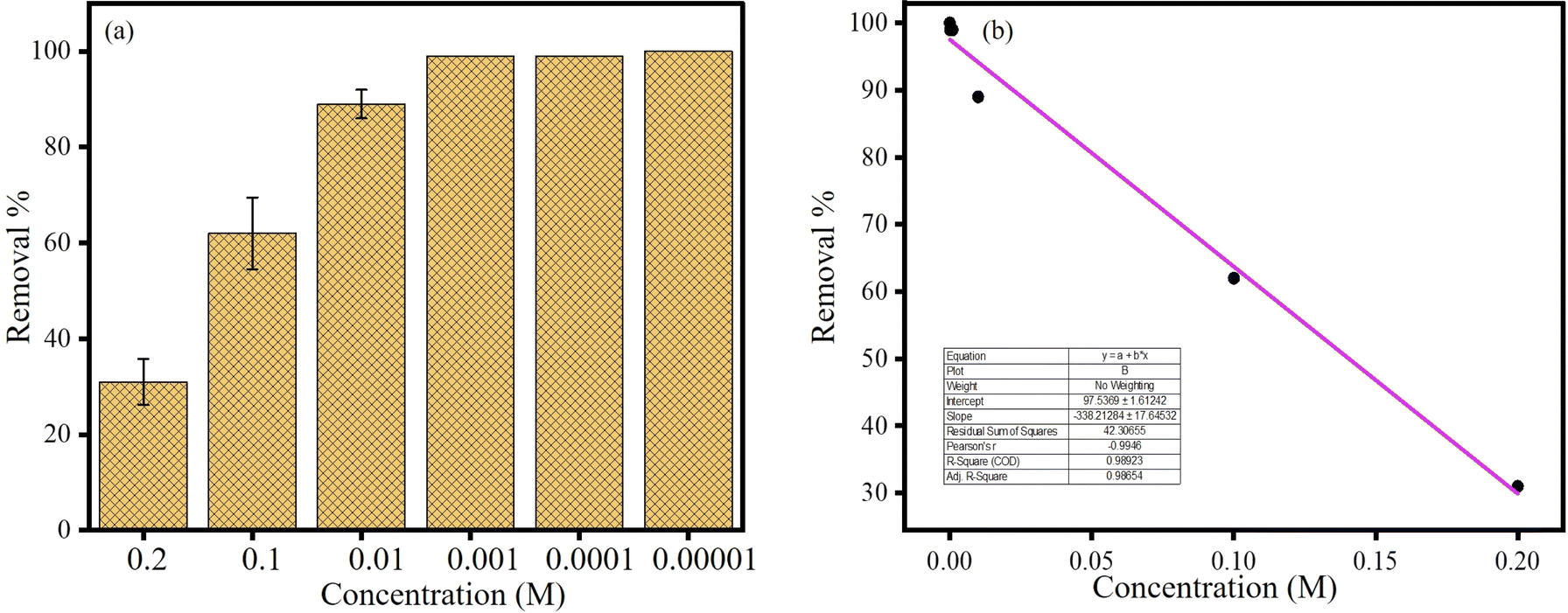

Fig. 9 (a) Bar diagram and (b) linear fit of % removal vs. [CR].

3.8 Colorimetric sensing of Hg²⁺

Not only fluorimetric sensing but also colorimetric sensing was performed employing CRAgOSA. Various metal ions (Pb²⁺, Ba²⁺, Na⁺, K⁺, Hg²⁺, K⁺, Zn²⁺, Cu²⁺, Al³⁺, Fe³⁺, Ni²⁺, Co²⁺, Ca²⁺, Mg²⁺, control) were employed in the CRAgOSA. No metal ion was able to change the color of the red-colored CRAgOSA solution except for Hg²⁺. Hg²⁺ selectively made the solution deep blue due to the simultaneous aggregation of AgNPs and complexation with CR induced by Hg²⁺. Such an observation helped us to design a colorimetric sensing platform for Hg²⁺ (LOD 1.36 × 10⁻⁵ and linear detection range from 1.00 × 10⁻⁴ to 5 × 10⁻⁷ M) (Fig. 10). FESEM images indicated that HgCRAgOSA (Hg²⁺ + CRAgOSA) had a flower shape, and the high-resolution FESEM identified the nanopetals of the flower (Fig. 11).

Fig. 10 (a) Digital image of the colorimetric sensing of Hg²⁺; (b) absorbance spectra of AgOSA + CR hydrosol with different metal ions. (c) Bar diagram of A/A₀ with different metal ions. (d) Plot of A/A₀vs. [Hg²⁺] and linear detection range of Hg²⁺ detection [A = absorbance of CRAgOSA with metal ions; A₀ = absorbance of CRAgOSA without metal ions].

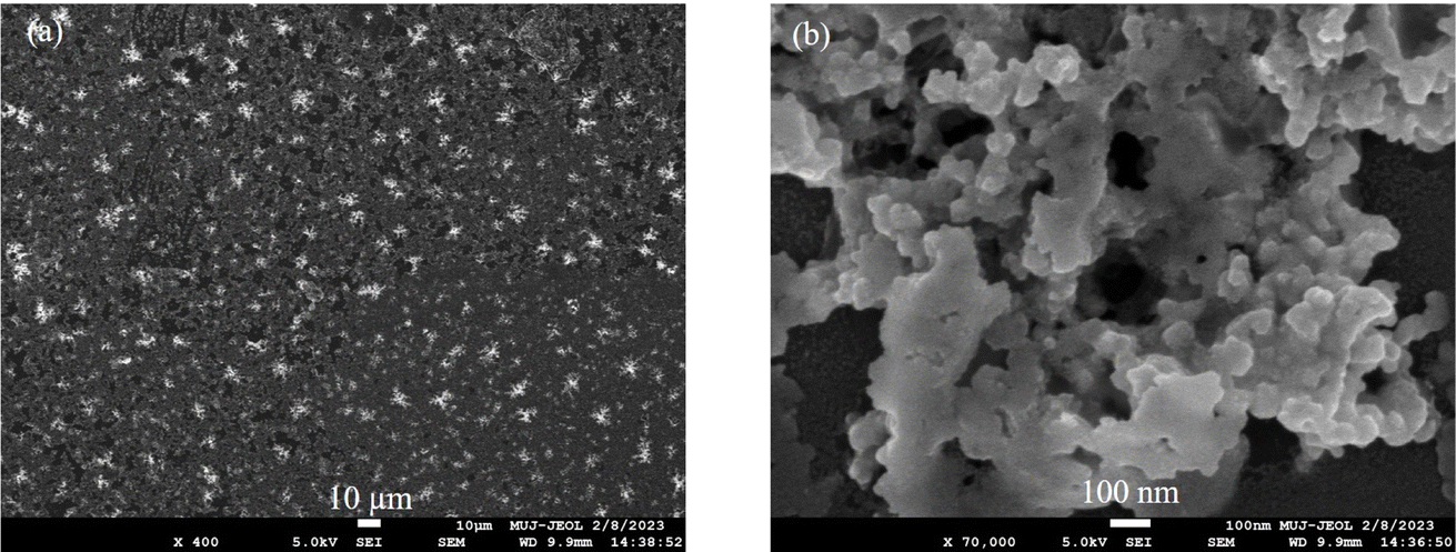Fig. 11 FESEM images of the precipitate after adding Hg²⁺ in CRAgOSA; (a) low resolution and (b) high resolution.

3.9 Estimation of Hg²⁺ in the natural sample

Hg²⁺ was estimated using our mentioned colorimetric protocol not only in distilled water (used in the laboratory) but also in natural water samples [Ganga water (Haridwar) rainwater (Jaipur), drinking water (Jaipur), tap water (Jaipur), and water from melted ice (Shimla)]. We added varying quantities of Hg²⁺ to the real water samples. The closeness to the actual spiking concentrations was achieved via the obtained colorimetric data (Table 3).

Table 3 Estimation of Hg²⁺ in various natural water samples

Sample name	Added [Hg^2+] (M)	[Hg^2+] detected (M)	Recovery (%)	Relative error (%)	RSD (%) (n = 3)
Ganga water (Haridwar)	5.00 × 10^−5	5.20 × 10^−5	104	4	0.4
	5.00 × 10^−4	4.84 × 10^−4	96.8	3.2	3.2
	5.00 × 10^−3	4.81 × 10^−3	96.2	3.8	3.1
Rainwater (Jaipur)	5.00 × 10^−5	4.84 × 10^−5	96.8	3.2	0.5
	5.00 × 10^−4	4.90 × 10^−4	98	2	0.9
	5.00 × 10^−3	5.21 × 10^−3	104.2	4.2	0.7
Drinking water (Jaipur)	5.00 × 10^−5	4.89 × 10^−5	97.8	2.2	2.3
	5.00 × 10^−4	5.03 × 10^−4	100.6	0.6	0.6
	5.00 × 10^−3	4.83 × 10^−3	96.6	3.4	1.2
Tap water (Jaipur)	5.00 × 10^−5	5.20 × 10^−5	104	4	1.2
	5.00 × 10^−4	5.08 × 10^−4	101.6	1.6	0.4
	5.00 × 10^−3	5.11 × 10^−3	102.2	2.2	0.9
Water from melted ice (Shimla)	5.00 × 10^−5	4.95 × 10^−5	99	1	0.9
	5.00 × 10^−4	5.05 × 10^−4	101	1	2.2
	5.00 × 10^−3	4.98 × 10^−3	99.6	0.4	1.4

---

3.10 Circular economy

Circular economy means adding value to waste materials and repurposing them to create expensive goods.⁴⁶ These wastes include scrap iron, algal biomass, and agro-industrial waste, which align with the circular economy's production tenets of removal (adsorption/degradation) and regeneration.

The denim industry is also investigating circular economy concepts to improve the sustainability of dyes. Reducing waste creation and resource consumption may be achieved by designing dyes and dyeing processes to make recycling and reuse simpler. Circular economy concepts are aligned with the implementation of closed-loop systems that collect, cure, and reuse dyes. The circular economy, decarbonization plans, and sustainable dyeing methods all help to make the denim industry's future more sustainable.⁴⁷

The toxic dye Congo red was eliminated employing Co²⁺ in quinone-capped silver hydrosol. As a corollary of dye adsorption, Co²⁺ sensing was made possible fluorometrically in one pot. Moreover, Hg²⁺ sensing was also made possible due to its unique interaction with CR. The protocol was cost-effective, fast, and energetically favorable (no external energy was employed). Thus, a model toxic dye was used for the recognition of poisonous metals along with the elimination of the toxic dye.

4. Conclusions

A highly luminescent silver hydrosol, obtained from salicylaldehyde, was used to eliminate Congo red and detect Co²⁺ and Hg²⁺. Fluorescence is a highly sensitive technique for the detection of an analyte. AgOSA was strongly fluorescent due to MEF. The strong affinity of CR and Ag, based on Ag–S interaction, resulted in the quenched fluorescence of AgOSA. Co²⁺ removed CR from the surface of Ag⁰ and accelerated MEF. Co²⁺ also released self-quenching. For AgOSA, the MEF was due to metallic silver. On the other hand, CoCRAgOSA exhibited MEF due to silver and cobalt with stronger fluorescence than AgOSA. Thus, Co²⁺ sensing was highly sensitive and selective. No other metal ions could show such type of turn-on fluorescence.

The use of the dye for the detection of harmful metals included the simultaneous use of metal-enhanced fluorescence and colorimetric route, marking the first instance of such a combination regarding circular economy. The process of environmental restoration and sensing was conducted in a single container, making it both cost-effective and efficient for practical prototype applications. Sulfur's affinity for Co²⁺ and the release of self-quenching were responsible for the restoration of fluorescence, while the complexation of CR with Hg²⁺ was the driving force behind colorimetric sensing. This type of work will hopefully be an asset for young scientists working on circular economy.

Data availability

All the data are included in the ESI.†

Author contributions

Mamta Sahu: writing – original draft, Mainak Ganguly: writing – review & editing, conceptualization, Priyanka Sharma: visualization, Ankita Doi: visualization.

Conflicts of interest

The authors declare that they have no known competing financial interests or personal relationships that could have appeared to influence the work reported in this paper.

Acknowledgements

The authors are thankful to Central Analytical Facilities (MUJ) and Sophisticated Analytical Instrument Facility (MUJ) for instrumental facilities.

References

1. Y. Jeong, Y. M. Kook, K. Lee and W. G. Koh, Biosens. Bioelectron., 2018, 111, 102–116.
2. M. Ganguly, J. Pal, C. Mondal, A. Pal and T. Pal, Dalton Trans., 2015, 44, 4370–4379.
3. M. T. Yaraki and Y. N. Tan, Chem.–Asian J., 2020, 15, 3180–3208.
4. S. Y. Tee and E. Ye, Mater. Adv., 2021, 2, 1507–1529.
5. N. Namazi Koochak, E. Rahbarimehr, A. Amirjani and D. Fatmehsari Haghshenas, Plasmonics, 2021, 16, 315–322.
6. M. Harja, G. Buema and D. Bucur, Sci. Rep., 2022, 12, 1–18.
7. Kiran, R. Bharti and R. Sharma, Mater. Today: Proc., 2021, 51, 880–885.
8. R. N. S. Bibi and R. L. Khan, World Appl. Sci. J., 2016, 34, 15–19.
9. J. H. Duffus, Pure Appl. Chem., 2002, 74, 793–807.
10. J. Briffa, E. Sinagra and R. Blundell, Heliyon, 2020, 6, e04691.
11. M. Sahu, M. Ganguly and P. Sharma, NanoWorld J., 2023, 9, 496–504.
12. A. Contino, G. Maccarrone, M. Zimbone, R. Riccardo, P. Musumeci, L. Calcagno and I. Oliveri, J. Colloid Interface Sci., 2016, 462, 216–222.
13. V. N. Mehta, A. K. Mungara and S. K. Kailasa, Anal. Methods, 2013, 5, 1818–1822.
14. J. L. MacLean, K. Morishita and J. Liu, Biosens. Bioelectron., 2013, 48, 82–86.
15. J. Huang, X. Mo, H. Fu, Y. Sun, Q. Gao, X. Chen, J. Zou, Y. Yuan, J. Nie and Y. Zhang, Sens. Actuators, B, 2021, 344, 130218.
16. M. Liu, Q. Zhang, T. Maavara, S. Liu, X. Wang and P. A. Raymond, Nat. Geosci., 2021, 14, 672–677.
17. H. Lade, S. Govindwar and D. Paul, Int. J. Environ. Res. Public Health, 2015, 12, 6894–6918.
18. F. Zarlaida and M. Adlim, Microchim. Acta, 2017, 184, 45–58.
19. K. Mohajershojaei, N. M. Mahmoodi and A. Khosravi, Biotechnol. Bioprocess Eng., 2015, 20, 109–116.
20. N. M. Mahmoodi, Water, Air, Soil Pollut., 2013, 224, 1612.
21. M. Ganguly and P. A. Ariya, ACS Omega, 2019, 4, 12107–12120.
22. M. Sahu, M. Ganguly and P. Sharma, Nanoscale Adv., 2024, 6, 4545–4566.
23. T. Liu, D. Li, D. Yang and M. Jiang, Langmuir, 2011, 27, 6211–6217.
24. M. H. Azarian, S. Nijpanich, N. Chanlek and W. Sutapun, RSC Adv., 2024, 14, 14624–14639.
25. A. Zielinska-jurek, E. Kowalska and J. W. Sobczak, Sep. Purif. Technol., 2010, 72, 309–318.
26. M. Sahu, M. Ganguly and A. Doi, ChemistrySelect, 2023, 8, e202301017.
27. J. R. Lakowicz, Plasmonics, 2006, 1, 5–33.
28. M. Ganguly, C. Mondal, J. Chowdhury, J. Pal, A. Pal and T. Pal, Dalton Trans., 2014, 43, 1032–1047.
29. J. R. Lakowicz, C. D. Geddes, I. Gryczynski, J. Malicka, Z. Gryczynski, K. Aslan, J. Lukomska, E. Matveeva, J. Zhang, R. Badugu and J. Huang, J. Fluoresc., 2004, 14, 425–441.
30. P. Prentø, Biotech. Histochem., 2009, 84, 139–158.
31. M. Yu, D. P. Woodruff, C. J. Satterley, R. G. Jones and V. R. Dhanak, J. Phys. Chem. C, 2007, 111, 3152–3162.
32. M. P. Jain and S. Kumar, Talanta, 1982, 29, 52–53.
33. K. Rajar, E. Alveroglu, M. Caglar and Y. Caglar, Mater. Chem. Phys., 2021, 273, 125082.
34. F. Mochi, L. Burratti, I. Fratoddi, I. Venditti, C. Battocchio, L. Carlini, G. Iucci, M. Casalboni, F. De Matteis, S. Casciardi, S. Nappini, I. Pis and P. Prosposito, Nanomaterials, 2018, 8, 1–14.
35. Y. Yao, D. Tian and H. Li, ACS Appl. Mater. Interfaces, 2010, 2, 684–690.
36. Y. Zhang, H. Wang, M. Lu, G. Li, M. Bai, W. Yang, W. Tan and G. Li, Chemosphere, 2024, 362, 142790.
37. H. Setyawati, H. Darmokoesoemo, I. K. Murwani, A. J. Permana and F. Rochman, Open Chem., 2020, 18, 287–294.
38. M. Ganguly, A. Pal and T. Pal, J. Phys. Chem. C, 2011, 115, 22138–22147.
39. Z. H. Xu, F. J. Chen, P. X. Xi, X. H. Liu and Z. Z. Zeng, J. Photochem. Photobiol., A, 2008, 196, 77–83.
40. H. Nishikawa and S. Yamada, Bull. Chem. Soc. Jpn., 1964, 37, 8–12.
41. M. Bartel, K. Markowska, M. Strawski, K. Wolska and M. Mazur, Beilstein J. Nanotechnol., 2020, 11, 620–630.
42. S. C. Petitto and M. A. Langell, J. Vac. Sci. Technol., A, 2004, 22, 1690–1696.
43. D.-H. Wu, M. U. Haq, L. Zhang, J.-J. Feng, F. Yang and A.-J. Wang, J. Colloid Interface Sci., 2024, 662, 149–159.
44. L.-L. Liu, D.-H. Wu, L. Zhang, J.-J. Feng and A.-J. Wang, J. Colloid Interface Sci., 2023, 639, 424–433.
45. C. D. Geddes, Phys. Chem. Chem. Phys., 2013, 15, 19537.
46. A. Doi, M. Ganguly and M. Sahu, Adsorption, 2024, 30, 425–441.
47. M. A. Yousaf and R. Aqsa, Global NEST J., 2023, 25, 39–51.

---

Footnote

† Electronic supplementary information (ESI) available: Fluorescence spectra, XPS, DRS, DLS, zeta, and bar diagram. See DOI: https://doi.org/10.1039/d4na00588k

---