
 Open Access Article
 This Open Access Article is licensed under a Creative Commons Attribution-Non Commercial 3.0 Unported Licence
nanoFeatures: a cross-platform application to characterize nanoparticles from super-resolution microscopy images†
Cristina
Izquierdo-Lozano
 ,
Niels
van Noort
,
Stijn
van Veen
,
Marrit M. E.
Tholen
,
Francesca
Grisoni
* and
Lorenzo
Albertazzi
*
,
Niels
van Noort
,
Stijn
van Veen
,
Marrit M. E.
Tholen
,
Francesca
Grisoni
* and
Lorenzo
Albertazzi
*
Department of Biomedical Engineering, Institute for Complex Molecular Systems (ICMS), Eindhoven University of Technology, 5612AZ Eindhoven, The Netherlands. E-mail: f.grisoni@tue.nl; l.albertazzi@tue.nl
First published on 16th October 2024
Abstract
Super-resolution microscopy and Single-Molecule Localization Microscopy (SMLM) are powerful tools to characterize synthetic nanomaterials used for many applications such as drug delivery. In the last decade, imaging techniques like STORM, PALM, and PAINT have been used to study nanoparticle size, structure, and composition. While imaging has progressed significantly, image analysis has often not advanced accordingly and many studies remain limited to qualitative and semi-quantitative analyses. Therefore, it is imperative to have a robust and accurate method to analyze SMLM images of nanoparticles and extract quantitative features from them. Here, we introduce nanoFeatures, a cross-platform Matlab-based app for the automatic and quantitative analysis of super-resolution images. nanoFeatures makes use of clustering algorithms to identify nanoparticles from the raw data (localization list) and extract quantitative information about size, shape, and molecular abundance at the single-particle and single-molecule levels. Moreover, it applies a series of quality controls, increasing data quality and avoiding artifacts. nanoFeatures, thanks to its intuitive interface, is also accessible to non-experts and will facilitate analysis of super-resolution microscopy for materials scientists and nanotechnologies. This easy accessibility to expansive feature characterization at the single particle level will bring us one step closer to understanding the relationship between nanostructure features and their efficiency (https://github.com/n4nlab/nanoFeatures).
1 Introduction
Nanoparticles have emerged as a promising tool in nanomedicine, owing to their remarkable physical and chemical properties.1,2 These physicochemical properties (e.g., size, shape, and the presence and quantity of surface ligands) are the key to selective delivery, via both passive,3 and active targeting.4 These approaches hold the potential to mitigate side effects and reduce the required drug dosage.1Despite these advantages, there has been limited success in translating nanoparticles to clinical applications. Since 1995, when Doxil became the first FDA-approved liposome-based nano-drug for cancer treatment,5 only 31 formulations have been clinically approved, including the emergency approval for the COVID-19 vaccine.6 The limited amount of approved nanoformulations shows that many open challenges still remain when translating the promising results of nanocarriers in vitro to a clinical application.7,8 Considering the vast number of nanoparticle formulations reported in the literature, this evidence highlights the urgent need for promoting the clinical approval of nanocarriers.
A current challenge is the lack of standardization in characterization methods, which results in a low degree of reliability and reproducibility in the nanomedicine literature.9 Properly characterizing nanoparticles is a fundamental step in their potential application, as their physical and chemical properties can differ vastly at the nanoscale. Morphological features, like size or shape, heavily influence the nanoparticle properties, leading to unforeseen behavior or even toxicity in the case of incorrect characterization.2,10 Currently available characterization techniques typically can only assess one property at a time, requiring the integration of multiple techniques for comprehensive characterization.2,11 Moreover, bulk measurement methods tend to average values and correspondingly mask the inherent heterogeneity of nanoparticles, which determines the effective distribution of nanoparticles to their site of action, and even their potential toxicity in biological media.10
Recently, super-resolution microscopy12 and, in particular, Single-Molecule Localization Microscopy (SMLM)13 have emerged as powerful techniques to improve nanoparticle characterization at the single-particle level. SMLM breaks the diffraction limit by computationally localizing individual fluorescent events separated in time and reconstructing super-resolved images based on these high-precision localizations. Therefore, SMLM images are created by stacking all the computed localization coordinates found in each frame of the acquisition movie, which allows researchers to visualize and analyze nanoparticles at the single-particle and single-molecule level with nanometer precision.13 This technique has already shown its versatility in various research fields from cell biology14,15 to material characterization,16,17 making it a powerful tool to address the challenges described above. For example, SMLM has been used to study and quantify protein corona formation on nanoparticles,18,19 which revealed their heterogeneous nature. Furthermore, by combining SMLM with Transmission Electron Microscopy (TEM), multidimensional information to describe this heterogeneity could be obtained.20 Moreover, SMLM has also allowed for the study of cell–nanoparticle interactions.21,22 Currently, research interest is shifting towards multiplexed images to correlate different modalities, which generate bigger datasets and complex data structures.23–27
A crucial side of SMLM is represented by data analysis, as it is the key to go from qualitative images to quantitative data. SMLM data analysis is based on: (1) processing the acquisition movie to obtain localizations, through the fitting of the point-spread function (PSF),28 (2) processing the localizations, for example, aligning or merging localizations,29 and finally (3) obtaining interpretable data30 that we can use to measure size and morphology, thanks to the high spatial resolution of SMLM (20–50 nm).13 Modular platforms like the Super-resolution Microscopy Analysis Platform (SMAP) allow the user to integrate many of the SMLM image analysis steps into single software.31 However, most of the available software resources are dedicated to biological imaging while materials and nanostructures lack tailored dedicated tools. A brief overview of multiple SMLM data analysis software can be found in ESI Table 3.† However most of these are meant for general image analysis, rather than a specialized characterization tool that runs on already processed localization data in batches. Therefore, these software solutions could complement the application presented in this work.
Here, we introduce nanoFeatures, an automated standalone MATLAB-based application dedicated to analyzing nanoparticles from SMLM datasets. The nanoFeatures app can process SMLM images, locate the nanoparticles, and automatically compute and display their features (Fig. 1). After simply uploading the raw datasets and setting the right parameters, the user will receive a list of the key features for each individual nanoparticle that can later be used in further analysis. By characterizing nanoparticles in a systematic and reproducible way, we aim to open the door for data-driven research, such as machine learning for property prediction or data mining. In what follows, we showcase an example application, whereby we analyse two different nanoparticle datasets: (1) dual color nanoparticles imaged with DNA-PAINT32 and (2) triple color nanoparticles imaged with exchange PAINT.23
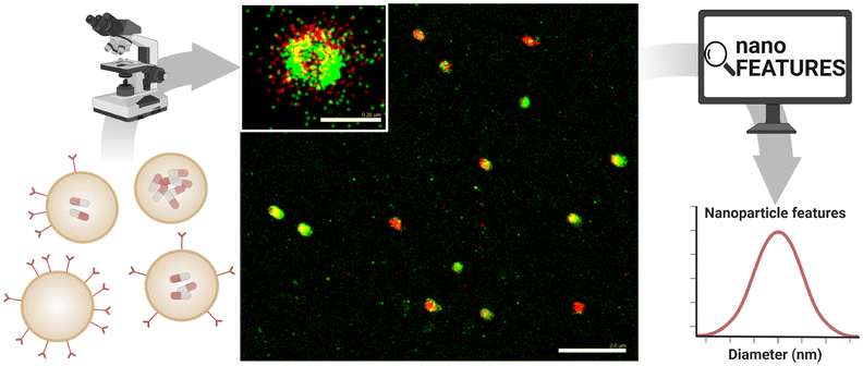 | ||
| Fig. 1 General nanoparticle analysis workflow. First, the nanoparticles are imaged in super-resolution microscopy. Then, the image data are sent to nanoFeatures to obtain nanoparticle features, such as size, shape, and number of binding sites. Scale bar 2 μm. | ||
2 Results and discussion
2.1 General procedure
A raw SMLM image is a list of coordinates for each of the fluorophore localizations found after fitting a Gaussian on the bright spots across the numerous frames in the acquisition movie (ESI Fig. 1†). An overview of the nanoFeatures algorithm is shown in Fig. 2a.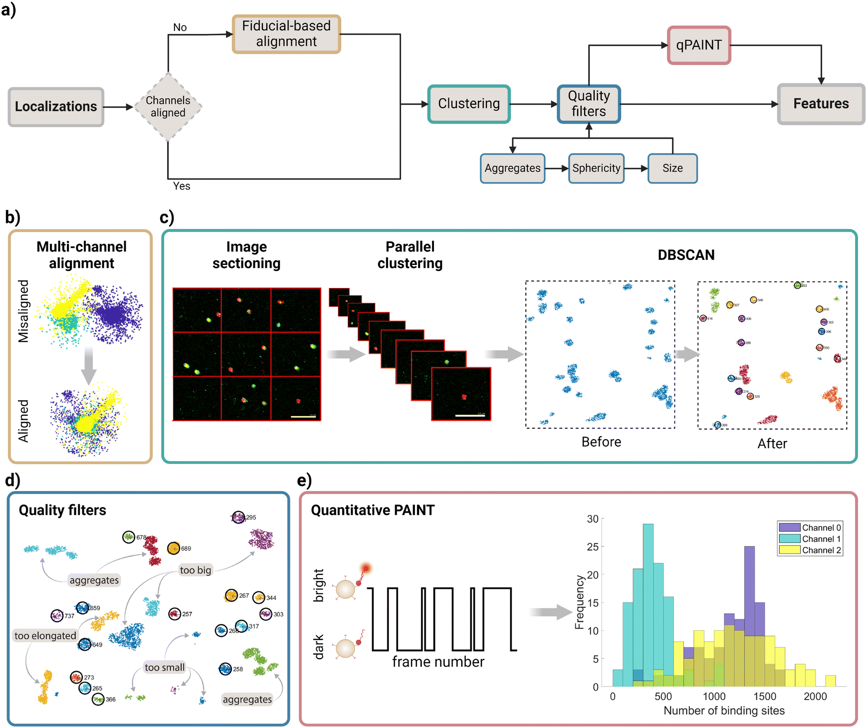 | ||
| Fig. 2 nanoFeatures algorithm. (a) General workflow from the raw dataset to the calculation of the nanoparticle's features. (b) Example of the channel alignment results, in this case aligning fiducials from three different channels. (c) Description of the image sectioning to send the different sections to parallel computing threads. MATLAB's DBSCAN is used to identify clusters in the sections, an example of how this algorithm works is also shown. Scale bar 2 μm. (d) Quality filters applied to the identified clusters by DBSCAN. Aggregated, non-spherical, or off-size nanoparticles are filtered in this step. Selected clusters are circled in black and given an ID number. (e) qPAINT scheme, the frames in which single fluorophores are on or off are counted, obtaining the dark and bright times, and are used to infer the total number of binding sites. | ||
The nanoFeatures general workflow is as follows (Fig. 2a):
(1) User input: several inputs are required from the user, which will determine the following steps of the analysis. The steps are as follows:
(a) File input. The user inputs the file, as specified in the User input subsection, containing the list of localization coordinates (ESI Fig. 1†). Multiple color channels can be input as a single file or as multiple files, corresponding to either simultaneous multi-color imaging (e.g. 2- or 3-color STORM) or sequential multiplexing (e.g. exchange-PAINT). To increase the throughput, users can select multiple files to be processed under the same settings in batch analysis.
(b) Input type selection. After inputting the file, the user must select the input type (ONI, NIKON, or ThunderSTORM), based on the microscope or software used to obtain the images.
(c) Workflow and parameter specification. Within the Graphical User Interface (GUI), users can specify the desired workflow for data processing. For example, when analyzing samples acquired sequentially, the user should activate the channel alignment option. Furthermore, users can define the parameters for filtering and feature extraction, and have the option to include the quantitative PAINT (qPAINT) analysis.33
(2) Read and pre-process file(s): once the input, workflow, and parameters have been defined, the data are pre-processed into a single list of localizations, containing all color channels.
(3) Channel alignment (optional) (Fig. 2b): if specified, the drift between different color channels is corrected before clustering.
(4) Clustering (Fig. 2c). The processed localizations are then used as the input of a clustering algorithm, which will identify potential nanoparticles, using the vicinity information.
(5) Quality filters (Fig. 2d): a series of quality filters are applied to exclude clusters of localizations not identified as single nanoparticles.
(6) qPAINT (optional) (Fig. 2e): quantifies the target ligands count based on the spatiotemporal response within each cluster.
(7) Generate output: finally, nanoFeatures will generate an output CSV file containing the features corresponding to each detected nanoparticle in the original SMLM image. This file, together with the plots prompted during the execution, will be saved in a “results” folder in the user's Matlab path.
In addition, SMLM images often have high background noise, leading to prolonged computing time for clustering analysis and complicating the automated identification of nanoparticles. For this reason, we advise pre-processing the image before using nanoFeatures, for example, by applying a density filter, as seen in ESI Fig. 2.† In this specific case study, we used the thunderSTORM plug-in for ImageJ,34 with the settings outlined in the Density filter subsection in Materials and methods. Moreover, a description of the datasets used for this case study can be found in the Datasets subsection in Materials and methods.
The following sections provide a detailed description of each of these steps.
2.2 User input
nanoFeatures accepts three distinct data structures, corresponding to outputs from various commercial microscopes or open-source image pre-processing software. The app extracts the pixel localizations (X, Y), the frame of detection, and the associated color channel. The three supported input file types are:(1) NIKON:35 TXT file format. The app reads the file as a table, identifying headers named “Channel_Name”, “X”, “Y” and “Frame”.
(2) ONI:36 comma-separated values (CSV) file format. The app reads the file as a matrix, considering the 1st column as the channel name, 2nd column as the frame number, and the 3rd and 4th columns as X and Y coordinates, respectively.
(3) ThunderSTORM:34 CSV file format. The app reads the file as a table, identifying headers named “Channel”, “Frame”, “x [nm]” and “y [nm]”.
Extension to further formats is envisioned in the future to follow the evolution of the different formats used in the community.
As an example, we showcase the workflow and parameter specification for the analysis of the file “210714_COOH_200_loc2_merge.csv”, which can be found in our online repository under the files “Datasets/dualColor/COOH_200nm_100dist_50neighbors”. The workflow and parameter selection can be seen in Fig. 3a–c and the results preview given by nanoFeatures within the GUI is seen in Fig. 3d.
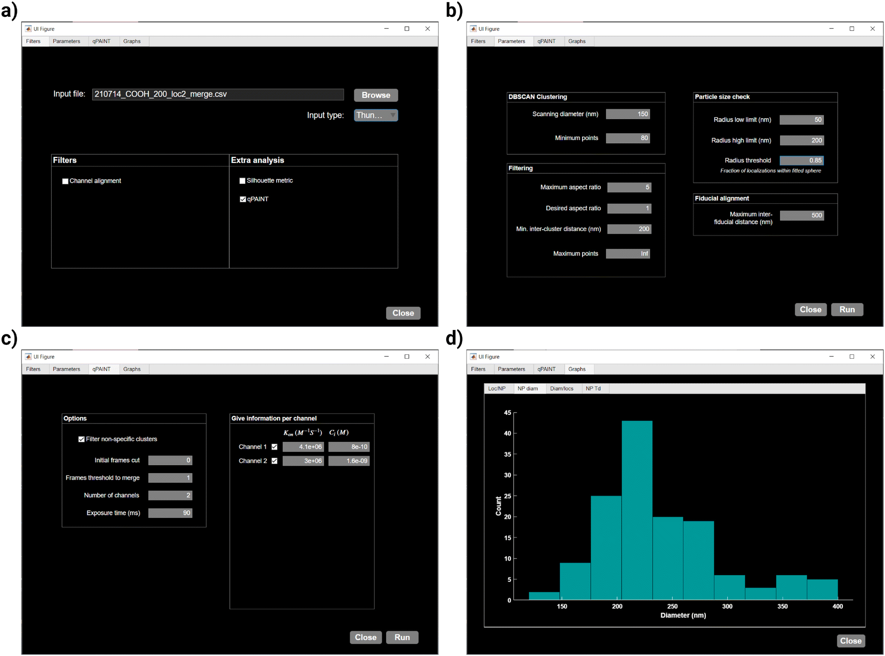 | ||
| Fig. 3 Case study using the nanoFeatures Graphical User Interface (GUI). (a) Filters tab to input the file(s) and select the desired filters, (b) parameters tab to input the specific parameters used to analyze the files, (c) qPAINT tab to input the parameters for the qPAINT analysis, if the checkbox is selected, and (d) graphs tab to show a preview of the results. | ||
2.3 Channel alignment
SMLM images are often acquired sequentially, one color at a time, such as through exchange-PAINT.23 The resulting data are stored in multiple localization files, one for each color. Since the image acquisition is done at different time points, there is a drift between the coordinates of different channels that we need to correct, as shown in Fig. 2b. To achieve this, we use fiducial markers—objects consistently visible in all color channels that serve as reference points. In this study, we use gold nanorods as fiducial markers.For this reason, upon clicking the “Run” button and only if the “channel alignment” checkbox is selected, nanoFeatures prompts the user to input files containing the fiducial localizations for each respective color channel.
To correct the temporal drift, first, the fiducial localizations are clustered to obtain their centroid. Then, nanoFeatures finds the n-channels nearest neighbors within a limited distance, to avoid fiducial mismatching. Finally, the average drift distances for each fiducial match between sequential files are calculated, after which the coordinates are corrected and the files are merged.
2.4 Clustering
After aligning all localizations from the different color channels and concatenating the files into a single matrix, the localizations are ready for clustering. This is a crucial step needed to identify individual nanoparticles and assign all the detected molecules to a specific nanoparticle or discard them as background.To speed up computational time, the image is divided into nine sections according to their coordinates. Then these sections are processed simultaneously in nCores − 1 ≤ 9 parallel computing threads, running the DBSCAN algorithm,37 as described in Fig. 2c. This parallelization step significantly reduces the execution time, while preventing the app from potential collapse due to the generation of massive data structures required to link all localizations within a background-dense image (ESI Fig. 3†). Note that at least one core remains available for other computer processes.
DBSCAN requires two parameters: (1) the radius in which adjacent localizations are considered as neighbors, and (2) the minimum number of points in this neighborhood required to form a cluster. These are introduced by the user, and they require optimization for each experiment and sample. To do this, the user can select the Silhouette checkbox in nanoFeatures to plot the Silhouette coefficient38 for each cluster, as in ESI Fig. 4f.† However, this analysis is computationally expensive, hence it is not recommended to use with large files or during batch analysis.
Then, nanoFeatures plots the reconstructed complete image (all nine sections), with the identified clusters by DBSCAN, which are depicted by different colors as shown in Fig. 4a.
 | ||
| Fig. 4 Selection of different figures obtained from nanoFeatures. (a) DBSCAN identified clusters and nanoparticles selected by the quality filters. (b) Selected nanoparticles colored based on the channel that each of the localizations was identified in. (c–f) Histograms showing the distribution for a few of the different features obtained from nanoFeatures. Graphs generated in MATLAB (a and b) and OriginLab (c–f), based on a 200 nm spherical nanoparticles sample. | ||
2.5 Quality filters
Although DBSCAN can identify clusters in images, and discard some localizations based on user-defined parameters, some quality filters are necessary to discard unwanted signals. For example, large aggregates or debris need to be discarded. Moreover, a strong background signal may be detected by DBSCAN as a particle. Therefore, to ensure that the identified clusters are indeed nanoparticles, the data undergo the following quality filters: (1) the sphericity filter removes clusters that are too elongated, or not elongated enough, depending on the sample. (2) The size filter removes clusters that are too big or too small. And (3) the aggregate filter removes clusters that are too close to each other (Fig. 2d).To do this, each filter (1) fits an ellipse on the clusters to obtain the aspect ratio, then (2) sets a random starting radius and adjusts it until a user-defined percentage of the cluster localizations fits in it, and finally, (3) ensures that the distance between each cluster centroid is at least the user-defined distance.
As a result of the quality filters, some clusters identified by DBSCAN are discarded, and only potential nanoparticles remain, marked by a black circle and an ID number in Fig. 4a. Additionally, nanoFeatures plots the selected nanoparticles from all nine sections, color-coded based on the localization channel. This way, users can identify co-localizing ligand populations on a nanoparticle (Fig. 4b).
At this point, within the GUI “Graphs” tab, nanoFeatures generates histograms providing an overview of nanoparticles’ characterization (Fig. 3d). For a more comprehensive analysis, users can plot the features from the generated CSV file, as showcased in Fig. 4c–f. For instance, these plots show features from a sample of 200 nm spherical nanoparticles.
Fig. 4c shows a wide distribution of nanoparticle diameters, peaking around 200 nm. Similarly, Fig. 4d shows the aspect ratio for the same sample, with its distribution mostly encompassed between 1 and 1.5, where 1 is a perfect sphere. These results align with the heterogeneous nature of nanoparticles, as described in the literature.10
2.6 qPAINT
Finally, if the sample was obtained following a DNA-PAINT protocol, users have the option to perform a quantitative PAINT (qPAINT) analysis33 (Fig. 2e). qPAINT allows researchers to determine the molecular abundance of the target in question. We used a previously published dataset17 to exemplify nanoFeatures’ usage. The sample is extensively described in section 4.1. Briefly, this consists of antibody-functionalized silica nanoparticles where the antibodies are targeted with DNA strands, enabling the counting and identification of antibodies on the nanoparticles’ surface. However, this method is not limited to DNA-based probes. For example, Riera et al. demonstrated the use of glycans as probes in a PAINT setup.39 By using super-resolution microscopy,40 and specifically PAINT, nanoparticles can be accurately characterized at the single-molecule level with a variety of probes,41–43 whereas other techniques like Scanning Electron Microscopy (SEM) provide excellent surface morphology imaging but lack the ability to quantify the presence of antibodies or other molecular components.First, the qPAINT filter generates a binary time trace for each identified cluster: bright (1), for each frame in which the fluorophores are active, or dark (0) when they are inactive.
Next, the user introduces the minimum number of frames that a cluster needs to be on (not dark), for the localizations to be merged into a single event. This number, the “frames threshold to merge”, needs to be optimized per sample, and it prevents false dark times.44 The duration of each dark time is then calculated by taking the derivative of the nanoparticle time traces and finding the difference between consecutive negative and positive changes. Clusters formed by non-specific localizations can be filtered by checking the corresponding checkbox within the GUI. Clusters will then be removed if their bright times do not comprise at least 50% of the total imaging time between their first and last binding events.
Furthermore, nanoFeatures constructs a cumulative distribution function (CDF) of the dark times for each remaining cluster, which is fitted with eqn (1), to obtain its mean dark time (τd*), where P represents the probability of a binding event at time t after a previous binding event (ESI Fig. 5†). Moreover, clusters are filtered on their CDF shape. When 90% of dark times are smaller than 10% of the longest dark time, the cluster is discarded.
| P(t) = 1 − e−t/τd* | (1) |
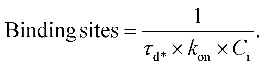 | (2) |
Then, τd*, in milliseconds, is used in eqn (2) to determine the number of binding sites per cluster (Fig. 4f). The association constant (kon) for each docking-imager pair and the imager concentration (Ci) are experiment-dependent.
Lastly, nanoFeatures will create a folder named “results” on the user's current Matlab path. This folder contains, for each file analyzed, most of the figures plotted by Matlab (ESI Fig. 4†) and a CSV file containing the number of binding sites, statistics of the bright and dark times, and R-squared for the exponential fit. A detailed list of all the features exported by nanoFeatures can be found in ESI, Table 2.†
3 Conclusion
nanoFeatures aims to fill the gap in standardizing nanoparticle characterization, particularly by analyzing super-resolution microscopy images. nanoFeatures achieves this by integrating multiple SMLM techniques, commercial microscopes and hardware set-ups, and diverse file formats. These can all be analyzed within the same algorithm, generating features organized in a unified data structure.In addition, nanoFeatures is an open-source platform, meaning that users can download and edit the source code of the app to add personalized functions and filters and even contribute to the public GitHub repository. Moreover, nanoFeatures is an app used daily within the research group; therefore, it is constantly updated (i.e., big fixing, new metrics, more plots, improved execution…), and will add more functionalities as they come.
Finally, despite being a Matlab-based application, the standalone version can be installed via MATLAB Runtime (without the need for a license), on multiple platforms like Linux, macOS, and Windows.
In this way, the many files generated from diverse experiments can be directly used in further analyses, minimizing or eliminating the need for extensive data pre-processing. For instance, employing machine learning to analyze various nanoparticle samples could provide valuable insights into the interrelationships of these features, thus aiding in the future design of nanoparticle formulations.
4 Materials and methods
4.1 Datasets
The results were obtained by analyzing two different datasets. The main dataset used depicts the different orientations of antibodies, fragment crystallizable (Fc) and antibody-binding fragment (Fab), on both carboxylic acid-activated silica (COOH) nanoparticle surface, and amino-functionalized silica (NH2) nanoparticle surface. Cetuximab (Ctx), an antibody targeting growth factor receptor, was conjugated to the COOH nanoparticles, resulting in a random orientation of the antibodies. On the other hand, to control the orientation of the antibodies in the NH2 nanoparticles, Fc-binding protein G and Fab-binding protein M were added to the nanoparticle's surface in different ratios, and then Ctx was immobilized on them in the selected orientation. Both Fab and Fc antibody orientations were imaged simultaneously with two different fluorophores (two color channels). The structure of this dataset consists of a list of localizations with information on their specific coordinates, frame number, and photon intensity. For more information on the synthesis and imaging of these nanoparticles, please refer to the article published by Marrit M. E. Tholen et al. (2023).17 To test the channel alignment filter, a DNA PAINT dataset consisting of both 300 nm polystyrene nanoparticles with conjugated ssDNA and 40 nm gold nanorod fiducials was used. The sample was measured at three different time points in multiple fields of view. These datasets, together with the nanoFeatures results, can be found in our online repository in Zenodo.Fig. 2b and e are based on the exchange PAINT files in the “tripleColor” folder. Fig. 4a and b are based on the file “210714_COOH_200_loc2_merge.csv” from Marrit Tholen's dataset and Fig. 4c–f are based on the combination of all files from sample “COOH_200nm”. These files can be found in the “dualColor” folder.
4.2 Drift correction
Fiducial markers can be used for drift correction due to the fact that they are stationary and permanently in an ‘on’ state. This was done in thunderSTORM, using a ‘minimum marker visibility ratio’ of 0.5, which means they should be on for at least half of the total frames to be considered as a fiducial marker. The ‘max distance [units of x, y]’, or the lateral tolerance for identification as a marker is usually set to 60.0 nm. The ‘trajectory smoothing factor’ is set to 0.5. When no fiducial markers are used, a cross-correlation function can be used.4.3 Fiducial localization files
Similarly, fiducials can also be identified by making use of the fact that they are permanently in an ‘on’ state. By applying an extreme density filter of 9000 minimum neighbors in a 50 nm radius, all nanoparticle clusters are filtered out and only the fiducials remain. This way, we can obtain the fiducial coordinates to be used within the channel alignment option.4.4 Density filter
Prior to analyzing the images in nanoFeatures, we used the thunderSTORM plug-in for ImageJ34 to remove the background noise. The settings are 100 nm radius and 60 minimum neighbors for sample COOH_100, 100 nm radius and 50 minimum neighbors for sample COOH_200, 100 nm radius and 100 minimum neighbors for sample COOH_300, and 100 nm radius and 50 minimum neighbors for sample NH2_200. Table 1 shows the files that were filtered with different settings.| File name | Radius (nm) | Minimum neighbors |
|---|---|---|
| 210714_COOH_200_loc1_merge | 100 | 80 |
| 210616_COOH_300_loc1_merge | 25 | 10 |
| 210616_COOH_300_loc2_merge | 50 | 10 |
| 210616_COOH_300_loc3_merge | 50 | 5 |
| 210616_COOH_300_loc3_merge | 50 | 10 |
| 210616_COOH_300_loc4_merge | 50 | 5 |
| 210616_COOH_300_loc5_merge | 50 | 5 |
| 210630_COOH_300_loc1_merge | 100 | 50 |
| 220103_COOH_300_pG_loc2_merge | 100 | 150 |
| 220103_COOH_300_pG_loc4_merge | 100 | 150 |
| 220103_COOH_300_pG_loc5_merge | 100 | 150 |
| 210812_NH2_75pG25pM_loc1_merge | 75 | 80 |
| 210812_NH2_75pG25pM_loc2_merge | 75 | 80 |
4.5 Hardware and software
In this work, nanoFeatures was run on MATLAB v. 2022b,45 on an AMD Ryzen 9 5900X 12-Core Processor 3.70 GHz with 32 GB RAM and a 64-bit Windows 10 Enterprise machine (Version 10.0.19045 Build 19045).Author contributions
Conceptualization: CIL, LA, and FG. Data curation: MMET, SvV, NvN, and CIL. Formal analysis: CIL, MMET, SvV, and NvN. Methodology: CIL, FG, and LA. Software: CIL, and NvN. Visualization: CIL. Writing – original draft: CIL. Writing – review and editing: all authors. All authors have approved the final version of the manuscript.Data availability
The code can be found on GitHub https://github.com/n4nlab/nanoFeatures, and the datasets used in Zenodo https://zenodo.org/records/10610875.Conflicts of interest
Biorender was used to design the figures in this work. The authors used ChatGPT as a tool to improve the readability and clarity of the manuscript, reviewed and edited the content as needed and take full responsibility for the content of the publication.Acknowledgements
The authors would like to thank Pietro del Canale and Roger Riera Brillas for the original scripts that nanoFeatures is based on and for engaging in algorithm discussions.Notes and references
- D. Peer, J. M. Karp, S. Hong, O. C. Farokhzad, R. Margalit and R. Langer, Nat. Nanotechnol., 2007, 2, 751–760 CrossRef CAS PubMed.
- N. Joudeh and D. Linke, J. Nanobiotechnol., 2022, 20, 262 CrossRef PubMed.
- A. K. Iyer, G. Khaled, J. Fang and H. Maeda, Drug Discovery Today, 2006, 11, 812–818 CrossRef CAS PubMed.
- R. Bazak, M. Houri, S. El Achy, S. Kamel and T. Refaat, J. Cancer Res. Clin. Oncol., 2015, 141, 769–784 CrossRef CAS PubMed.
- Y. C. Barenholz, J. Controlled Release, 2012, 160, 117–134 CrossRef CAS PubMed.
- A. C. Anselmo and S. Mitragotri, Bioeng. Transl. Med., 2021, 6, e10246 CrossRef CAS PubMed.
- J. M. Metselaar and T. Lammers, Drug Delivery Transl. Res., 2020, 10, 721–725 CrossRef PubMed.
- C. Zhang, L. Yan, X. Wang, S. Zhu, C. Chen, Z. Gu and Y. Zhao, Nano Today, 2020, 35, 101008 CrossRef CAS.
- S. Sharifi, N. N. Mahmoud, E. Voke, M. P. Landry and M. Mahmoudi, Nano-Micro Lett., 2022, 14, 172 CrossRef CAS PubMed.
- J.-M. Rabanel, V. Adibnia, S. F. Tehrani, S. Sanche, P. Hildgen, X. Banquy and C. Ramassamy, Nanoscale, 2019, 11, 383–406 RSC.
- D. Titus, E. James Jebaseelan Samuel and S. M. Roopan, Green Synthesis, Characterization and Applications of Nanoparticles, Elsevier, 2019, pp. 303–319 Search PubMed.
- C. G. Galbraith and J. A. Galbraith, J. Cell Sci., 2011, 124, 1607–1611 CrossRef CAS PubMed.
- M. Lelek, M. T. Gyparaki, G. Beliu, F. Schueder, J. Griffié, S. Manley, R. Jungmann, M. Sauer, M. Lakadamyali and C. Zimmer, Nat. Rev. Methods Primers, 2021, 1, 1–27 CrossRef.
- S. Liu, P. Hoess and J. Ries, Annu. Rev. Biophys., 2022, 51, 301–326 CrossRef CAS PubMed.
- L. Woythe, M. M. E. Tholen, B. J. H. M. Rosier and L. Albertazzi, ACS Appl. Bio Mater., 2023, 6, 171–181 CrossRef CAS PubMed.
- S. Pujals, N. Feiner-Gracia, P. Delcanale, I. Voets and L. Albertazzi, Nat. Rev. Chem., 2019, 3, 68–84 CrossRef.
- M. M. E. Tholen, B. J. H. M. Rosier, R. T. Vermathen, C. A. N. Sewnath, C. Storm, L. Woythe, C. Izquierdo-Lozano, R. Riera, M. van Egmond, M. Merkx and L. Albertazzi, ACS Nano, 2023, 17, 11665–11678 CrossRef CAS PubMed.
- N. Feiner-Gracia, M. Beck, S. Pujals, S. Tosi, T. Mandal, C. Buske, M. Linden and L. Albertazzi, Small, 2017, 13, 1701631 CrossRef PubMed.
- Y. Wang, P. E. D. Soto Rodriguez, L. Woythe, S. Sánchez, J. Samitier, P. Zijlstra and L. Albertazzi, ACS Appl. Mater. Interfaces, 2022, 14, 37345–37355 CrossRef CAS PubMed.
- T. Andrian, P. Delcanale, S. Pujals and L. Albertazzi, Nano Lett., 2021, 21, 5360–5368 CrossRef CAS PubMed.
- D. van der Zwaag, N. Vanparijs, S. Wijnands, R. De Rycke, B. G. De Geest and L. Albertazzi, ACS Appl. Mater. Interfaces, 2016, 8, 6391–6399 CrossRef CAS PubMed.
- S. Chen, J. Wang, B. Xin, Y. Yang, Y. Ma, Y. Zhou, L. Yuan, Z. Huang and Q. Yuan, Anal. Chem., 2019, 91, 5747–5752 CrossRef CAS PubMed.
- R. Jungmann, M. S. Avendaño, J. B. Woehrstein, M. Dai, W. M. Shih and P. Yin, Nat. Methods, 2014, 11, 313–318 CrossRef CAS PubMed.
- T. Ku, J. Swaney, J.-Y. Park, A. Albanese, E. Murray, J. H. Cho, Y.-G. Park, V. Mangena, J. Chen and K. Chung, Nat. Biotechnol., 2016, 34, 973–981 CrossRef CAS PubMed.
- M. Klevanski, F. Herrmannsdoerfer, S. Sass, V. Venkataramani, M. Heilemann and T. Kuner, Nat. Commun., 2020, 11, 1552 CrossRef CAS PubMed.
- F. Civitci, J. Shangguan, T. Zheng, K. Tao, M. Rames, J. Kenison, Y. Zhang, L. Wu, C. Phelps, S. Esener and X. Nan, Nat. Commun., 2020, 11, 4339 CrossRef CAS PubMed.
- E. M. Unterauer, S. S. Boushehri, K. Jevdokimenko, L. A. Masullo, M. Ganji, S. Sograte-Idrissi, R. Kowalewski, S. Strauss, S. C. M. Reinhardt, A. Perovic, C. Marr, F. Opazo, E. F. Fornasiero and R. Jungmann, Cell, 2024, 187-7, 1785–1800 CrossRef PubMed.
- A. Small and S. Stahlheber, Nat. Methods, 2014, 11, 267–279 CrossRef CAS PubMed.
- A. Balinovic, D. Albrecht and U. Endesfelder, J. Phys. D: Appl. Phys., 2019, 52, 204002 CrossRef CAS.
- K. J. A. Martens, B. Turkowyd and U. Endesfelder, Front. Bioinform., 2022, 1, 817254 CrossRef PubMed.
- J. Ries, Nat. Methods, 2020, 17, 870–872 CrossRef CAS PubMed.
- J. Schnitzbauer, M. T. Strauss, T. Schlichthaerle, F. Schueder and R. Jungmann, Nat. Protoc., 2017, 12, 1198–1228 CrossRef CAS PubMed.
- R. Jungmann, M. S. Avendaño, M. Dai, J. B. Woehrstein, S. S. Agasti, Z. Feiger, A. Rodal and P. Yin, Nat. Methods, 2016, 13, 439–442 CrossRef CAS PubMed.
- M. Ovesný, P. Křížek, J. Borkovec, Z. Švindrych and G. M. Hagen, Bioinformatics, 2014, 30, 2389–2390 CrossRef PubMed.
- N-STORM, https://www.microscope.healthcare.nikon.com/products/super-resolution-microscopes/n-storm-super-resolution.
- ONI, https://oni.bio/.
- E. Schubert, J. Sander, M. Ester, H. P. Kriegel and X. Xu, ACM Trans. Database Syst., 2017, 42, 1–21 CrossRef.
- P. J. Rousseeuw, J. Comput. Appl. Math., 1987, 20, 53–65 CrossRef.
- R. Riera, T. P. Hogervorst, W. Doelman, Y. Ni, S. Pujals, E. Bolli, J. D. Codée, S. I. van Kasteren and L. Albertazzi, Nat. Chem. Biol., 2021, 17, 1281–1288 CrossRef CAS PubMed.
- S. Dhiman, T. Andrian, B. S. Gonzalez, M. M. Tholen, Y. Wang and L. Albertazzi, Chem. Sci., 2022, 13, 2152–2166 RSC.
- M. M. Tholen, R. P. Tas, Y. Wang and L. Albertazzi, Chem. Commun., 2023, 59, 8332–8342 RSC.
- R. P. Tas, L. Albertazzi and I. K. Voets, Nano Lett., 2021, 21, 9509–9516 CrossRef CAS PubMed.
- E. Archontakis, L. Deng, P. Zijlstra, A. R. Palmans and L. Albertazzi, J. Am. Chem. Soc., 2022, 144, 23698–23707 CrossRef CAS PubMed.
- R. Riera, E. Archontakis, G. Cremers, T. de Greef, P. Zijlstra and L. Albertazzi, ACS Sens., 2023, 8, 80–93 CrossRef CAS PubMed.
- R2022b – Updates to the MATLAB and Simulink product families, https://nl.mathworks.com/products/new_products/release2022b.html.
Footnote |
| † Electronic supplementary information (ESI) available. See DOI: https://doi.org/10.1039/d4nr02573c |
| This journal is © The Royal Society of Chemistry 2024 |