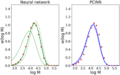
Polymer chemistry informed neural networks (PCINNs) for data-driven modelling of polymerization processes†
Nicholas
Ballard
 *ab,
Jon
Larrañaga
a,
Kiarash
Farajzadehahary
 a and
José M.
Asua
a
aPOLYMAT – University of the Basque Country UPV/EHU, Joxe Mari Korta zentroa, Tolosa Hiribidea 72, Donostia-San Sebastián 20018, Spain. E-mail: nicholas.ballard@polymat.eu
bIKERBASQUE, Basque Foundation for Science, Plaza Euskadi 5, 48009 Bilbao, Spain
First published on 30th October 2024
Abstract
Although the use of neural networks is now widespread in many practical applications, their use as predictive models in scientific work is often challenging due to the high amounts of data required to train the models and the unreliable predictive performance when extrapolating outside of the training dataset. In this work, we demonstrate a method by which our knowledge of polymerization processes in the form of kinetic models can be incorporated into the training process in order to overcome both of these problems in the modelling of polymerization reactions. This allows for the generation of accurate, data-driven predictive models of polymerization processes using datasets as small as a single sample. This approach is demonstrated for an example solution polymerization process where it is shown to significantly outperform purely inductive learning systems, such as conventional neural networks, but can also improve predictions of existing first principles kinetic models.
Introduction
The physical properties of polymers are governed by the composition of the polymer and their macromolecular structure, both of which are largely determined during synthesis.1,2 As a result, significant effort has been put into understanding the nature of polymerization processes, and how polymerization conditions can be adjusted during the reaction to achieve a desired product. In the field of polymer reaction engineering, this is commonly achieved by generating population balance models that consider the evolution of the different species in the reaction as a function of the various chemical reactions that can occur.3–5 Such models have proven to be incredibly useful in understanding polymerization processes, and have helped guide research in practical applications such as process design and control.6–11Despite the clear utility of kinetic models, they often struggle to accurately describe all aspects of a dataset quantitatively. When proposed for use in control of polymerization reactors, this leads to challenges in reliably reaching a given target macromolecular composition. Often this lack of accuracy may be attributed to errors in assumed rate coefficients or deliberate choices in the model, such as assumptions that are made to limit model complexity. However, in many cases the challenges in making accurate predictions across a wide range of conditions may simply be the result of omission of some reaction that is not currently known, or batch-to-batch variations that are hard to model physically.
As an alternative to first principles kinetic models, which seek to make predictions based on a fundamental understanding of the process, data-driven techniques can be used.12–15 Of the various data-driven techniques that can be applied, neural networks are particularly attractive due to their flexibility and their ability to be scaled.16 Neural networks are parametric models, whose parameters (or weights) are adjusted during training to maximize the accuracy of prediction on a given training dataset. Unfortunately, the way in which neural networks are typically trained will inevitably bring about two major issues when applied to modelling polymerization processes. First, the large number of parameters in a typical neural network means that the data requirements for an accurate predictive model are far beyond what is typically available experimentally. Second, as neural networks do not have any fundamental understanding of the underlying function they are approximating, both interpolation and, more importantly, extrapolation to make predictions outside of the training dataset can result in significant errors. As a result of these drawbacks, when applied to polymer science, the majority of work on data-driven modelling has focussed on the relatively limited set of problems where large datasets exist.17–21
In this work we seek to overcome these issues and develop predictive models based on neural networks that leverage both the theoretical understanding of the underlying chemistry involved in the polymerization process and the available data. To understand how this may be achieved, we may consider a simple example as shown in Fig. 1. Fig. 1 shows a series of four (x,y) points which are drawn from simple polynomial expression (y = −18x4 + 35x3 − 21x2 + 4.4x evaluated at x = 0, 0.3, 0.6 and 0.95). In terms of a data-driven approach, such as a neural network, this would be modelled by a network with one input unit (x) and one output unit (y). The conventional way of training is to adjust the parameters of the network to minimize the predictive error, which is measured in terms of what in the machine learning community is referred to as the loss function (this is known as the objective function in some other fields). For a conventional neural network, the loss function (L) may be represented by the mean square error:
 | (1) |
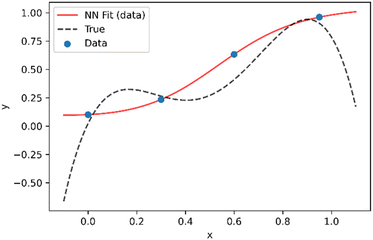 | ||
| Fig. 1 Example of a neural network model (red line) fit to a series of four (x,y) data points extracted from an underlying distribution given by y = −18x4 + 35x3 − 21x2 + 4.4x (dotted black line). | ||
Looking at the results from Fig. 1, two obvious issues can be observed. The first is that although the training data is perfectly fit, predictive performance between training data points (interpolation) is relatively poor. This can be avoided by using larger training datasets but becomes an increasingly important issue with high dimensional data (i.e. for systems with a large number of inputs). The second major issue that arises is that predictive performance outside the region of the training dataset (extrapolation) is very poor.
The method used here to overcome these issues is to incorporate some knowledge we may have of the underlying function into the training process, similar to the “explanation based neural networks” of Thrun and coworkers23,24 and the “tangent prop” algorithm of Simard et al.25 Taking the example from Fig. 1, let us imagine that we have some prior knowledge that the function is a 4th order polynomial expression and a reasonable, but imperfect, guess of the polynomial coefficients. This knowledge can be incorporated by ensuring that, in addition to minimizing the predictive error, the neural network mimics the trends expected from the theoretical function. To do so, the loss function is adapted to include a data driven component as in eqn (1) and an additional component that incorporates prior knowledge in the form of derivatives such that:
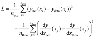 | (2) |
 is the derivative extracted from the neural network for input xj and
  is the derivative obtained from the theoretical function that is assumed for input xj. Note that values of xj can be taken anywhere such that the gradient can be forced to fit over a much wider range of values that the available experimental data points. With this new loss function, during training the parameters of the network can now be adjusted to minimize the predictive error as well as the error in the gradients.23,24
As shown in Fig. 2, even if the assumed theoretical function is not completely correct, incorporation of the derivatives into the loss function, results in a neural network that is a much better approximation of the true function, such that both interpolation and extrapolation performance are improved.
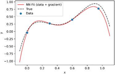 | ||
| Fig. 2 Demonstration of approach to combine data and theory in training neural network. As opposed to Fig. 1, in addition to the data points it is assumed that the data follows a trend represented by y = −23x4 + 47x3 − 20x2 + 6.6x which is used to supply the values of dy/dxtheo in eqn (2). | ||
It may be noted that recently the incorporation of theoretical knowledge into the loss functions of neural networks has been employed to generate neural network models that are constrained to give physically realistic models. These “physics informed neural networks” (PINNs) take a similar approach to that described above but ensure that the derivative terms are in agreement with underlying physical laws.26,27 Implementing these kind of “informed” machine learning systems is particularly interesting in the case of problems in polymer chemistry where the processes are complex and datasets are limited, but a significant amount of fundamental knowledge about the chemistry involved is known.
In this paper, we describe the development of neural networks that take advantage of our knowledge of polymerization processes in the form of kinetic models. This fundamental knowledge is combined with data-driven approaches to generate Polymer Chemistry Informed Neural Networks (PCINNs) capable of accurate prediction of polymerization reactions. As an example of the implementation, the case of solution polymerization of methyl methacrylate is discussed in which a small experimental dataset of just 8 reactions is used. First, a simple case where only the prediction of the evolution of conversion is desired is described. Subsequently, a more complex example where the evolution of conversion, molar mass and the full molecular weight distribution is shown. Finally, the potential use of such data-driven models for online forecasting of polymerization reactions is demonstrated.
Experimental
Materials
Methyl methacrylate (MMA, Quimidroga, technical grade) toluene (Sigma Aldrich, ACS reagent grade) and 2,2′-azobis(2-methylpropionitrile) (AIBN, Sigma Aldrich, 98%) were used as received.Synthesis
In a typical polymerization reaction (R1), a solution of MMA (49.9 g) in toluene (94.9 g) was prepared in a round bottomed flask fitted with a reflux condenser and a magnetic stirrer bar. Nitrogen was passed through the solution for 15 minutes and then the reaction vessel was immersed in an oil bath at the desired temperature (60 °C). After 15 minutes a solution of AIBN (0.61 g) in toluene (5 g) was added to initiate the reaction. During the reaction, samples were taken and cooled to ambient temperature for subsequent conversion and molecular weight analysis. Full details of the reactions carried out are given in Table 1.| Reaction code | Reaction temperature (°C) | Monomer (g) | Initiator (g) | Toluene (g) |
|---|---|---|---|---|
| R1 | 60 | 49.9 | 0.61 | 99.9 |
| R2 | 70 | 50.0 | 0.30 | 100.1 |
| R3 | 60 | 25.0 | 0.92 | 100.0 |
| R4 | 70 | 10.3 | 0.90 | 100.0 |
| R5 | 80 | 25.0 | 0.30 | 100.0 |
| R6 | 80 | 10.0 | 0.60 | 100.0 |
| R7 | 70 | 25.1 | 0.60 | 100.0 |
| R8 | 80 | 50.0 | 0.90 | 100.1 |
Characterization
During the polymerization, samples were extracted from the reactor and the monomer conversion was determined gravimetrically.The molecular weight distributions (MWD) were measured using size exclusion chromatography (SEC). The GPC instrument consisted of an injector, a pump (Waters 510), three columns in series (Styragel HR2, HR4, and HR6), and a differential refractometer detector (Waters 2410). The equipment was calibrated using polystyrene standards. The THF flow rate was set at 1 mL min−1. The reported molar masses were determined by comparing them with polystyrene standards.
Mathematical model
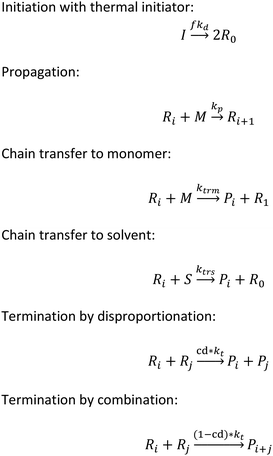
To implement the mathematical model for the solution polymerization of methyl methacrylate, the reactions shown in Scheme 1 were considered. The rate coefficients for the various reactions were taken from literature and are shown in Table 2. Due to the relatively high concentrations of solvent used in this work, no gel effect was considered in the kinetic model. In the case of chain transfer to monomer, the Arrhenius parameters were not available and therefore a fixed ratio of ktrm/kp of 5.27 × 10⁻⁵ was used.28 The implementation of the model was performed using the method described by Morbidelli and coworkers.29 Due to the computational challenges in calculating the full molecular weight distribution, the model makes use of the discretization method of Kumar and Ramkrishna30 and separates the molecular weight distribution into a smaller number of “pivots”. For the molecular weight distribution 30 pivots were used separated on a logarithmic scale up to a maximum of 50![[thin space (1/6-em)]](https://www.rsc.org/images/entities/char_2009.gif) 000 monomer units. In order to facilitate the training of neural networks capable of predicting the molecular weight distributions, fixed pivots were used.
000 monomer units. In order to facilitate the training of neural networks capable of predicting the molecular weight distributions, fixed pivots were used.
Initiation with thermal initiator:
Propagation:
Chain transfer to monomer:
Chain transfer to solvent:
Termination by disproportionation:
Termination by combination:
Computational methods
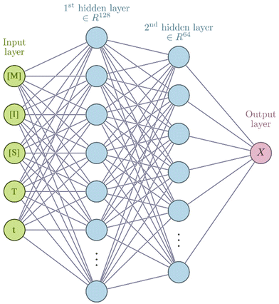
Neural network models were developed using the PyTorch framework36 (version 2.0.1) in Python (version 3.9.18) using a standard desktop PC (Intel Core i7-7700 CPU, 32 GB RAM).For the neural networks trained using experimental data, training was performed using a learning rate of 3 × 10⁻⁴ for 10![[thin space (1/6-em)]](https://www.rsc.org/images/entities/char_2009.gif) 000 epochs using the ADAM optimizer. Each epoch corresponds to computing the loss function on the entire experimental data set and adjusting the parameters accordingly by a value determined by the learning rate. The number of epochs chosen corresponds roughly to the point where further training does not improve the loss of the training set. The mean square error was used for the loss function. Due to the relatively small size of the dataset, a leave-one-experiment-out strategy was used to split the train and test dataset, whereby 8 separate models were trained in which the training set was 7/8 experiments and the remaining experiment was used for the test set. The neural networks have 5 inputs: concentration of monomer [M], initiator [I], solvent [S], temperature (T) and reaction time (t). All inputs were scaled individually to values between 0 and 1. There are two hidden layers in the network of 128 and 64 units respectively. In the hidden layers a so-called activation function is generally used to introduce non-linearity such that complex relationships between input data can be learnt. In this network the hyperbolic tangent activation function (eqn (3)) was used.
000 epochs using the ADAM optimizer. Each epoch corresponds to computing the loss function on the entire experimental data set and adjusting the parameters accordingly by a value determined by the learning rate. The number of epochs chosen corresponds roughly to the point where further training does not improve the loss of the training set. The mean square error was used for the loss function. Due to the relatively small size of the dataset, a leave-one-experiment-out strategy was used to split the train and test dataset, whereby 8 separate models were trained in which the training set was 7/8 experiments and the remaining experiment was used for the test set. The neural networks have 5 inputs: concentration of monomer [M], initiator [I], solvent [S], temperature (T) and reaction time (t). All inputs were scaled individually to values between 0 and 1. There are two hidden layers in the network of 128 and 64 units respectively. In the hidden layers a so-called activation function is generally used to introduce non-linearity such that complex relationships between input data can be learnt. In this network the hyperbolic tangent activation function (eqn (3)) was used.
 | (3) |
Although the ultimate goal of the PCINN is to predict the full molecular weight distribution, accurate prediction of each point of the distribution is challenging, therefore, in the outputs of the model, the moments of the distribution expressed as average molecular weights were considered. Therefore, the final output is a layer of 6 units (conversion, log10(Mn), log10(Mw), log10(Mz), log10(Mz+1) and log10(Mv)) with no activation function used. The number-average (Mn), weight-average (Mw), z-average (Mz), (z + 1)-average (Mz+1), and viscosity-average molecular weights (Mv) are defined by
 | (4) |
 | (5) |
 | (6) |
 | (7) |
 | (8) |
A value of a = 0.704 was used in the calculation of the viscosity average molecular weight.
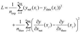
In the case of PCINNs, in addition to the data driven component used in the loss function, in each epoch of training, a separate theoretical model was used to calculate the Jacobian with respect to the input values for a batch of 32 randomly sampled values of [M], [I], [S], temperature and reaction time. The values of the Jacobian elements were then used in the loss function shown in eqn (9)
 | (9) |
 corresponds to the elements of the Jacobian extracted from the neural network for input xj and
  corresponds to the elements of the Jacobian extracted from the theoretical model (see below). Note that random samples were used in the Jacobian calculations which means that the derivative terms are different in each iteration (epoch) of the training of the NN.
Although the first principles mathematical model described in the previous section could in principle be used to estimate the theoretical Jacobian, this would involve extensive computational effort. In order to avoid this, and taking advantage of the fact that the outputs of neural networks are directly differentiable with respect to the inputs, in this work a separate neural network model was built using the data from a first principles mathematical model to train and the components of the Jacobian were then directly obtained from the NN model.
For this “theory” neural network, 10![[thin space (1/6-em)]](https://www.rsc.org/images/entities/char_2009.gif) 000 simulated reactions were performed to generate the data by using the mathematical model described above with a random reaction time ranging between 5 min to 10 h, a reaction temperature ranging between 50 and 90 °C, a monomer concentration ranging between 5 and 0.5 mol L−1 and an initiator concentration ranging between 0.1 mol L−1 and 0.005 mol L−1. For each simulated reaction 250 points were sampled during the reaction time at which point the conversion and the molecular weight distribution were logged. The total simulation time for all simulated reactions was around 3 days. The data was split so that the first 95% of simulated reactions were used for training data, and 5% of data was held back for use in the test set. Similar to the network described above, the theory neural network has 5 inputs ([M], [I], [S], T and t). All inputs were scaled individually to values between 0 and 1. There are three hidden layers of 128, 64 and 64 units respectively that use the rectified linear unit (ReLU) activation function (eqn (10)).
000 simulated reactions were performed to generate the data by using the mathematical model described above with a random reaction time ranging between 5 min to 10 h, a reaction temperature ranging between 50 and 90 °C, a monomer concentration ranging between 5 and 0.5 mol L−1 and an initiator concentration ranging between 0.1 mol L−1 and 0.005 mol L−1. For each simulated reaction 250 points were sampled during the reaction time at which point the conversion and the molecular weight distribution were logged. The total simulation time for all simulated reactions was around 3 days. The data was split so that the first 95% of simulated reactions were used for training data, and 5% of data was held back for use in the test set. Similar to the network described above, the theory neural network has 5 inputs ([M], [I], [S], T and t). All inputs were scaled individually to values between 0 and 1. There are three hidden layers of 128, 64 and 64 units respectively that use the rectified linear unit (ReLU) activation function (eqn (10)).
| ReLU(x) = max(0,x) | (10) |
The final output splits to give one output neuron for conversion on which the sigmoid activation function was used. The sigmoid function constrains the output to be between 0 and 1 according to eqn (11).
 | (11) |
Another series of output units that predict log10(Mn), log10(Mw), log10(Mz), log10(Mz+1) and log10(Mv) using the softplus activation function was used. The softplus function (eqn (12)) prevents negative values being returned.
| softplus(x) = ln(1 + ex) | (12) |
Training was performed using a learning rate of 5 × 10⁻⁵ for 25 epochs using the ADAM optimizer. The mean square error was used for the loss function. Predictive performance in this case is essentially perfect as shown in Fig. S1.† The average mean squared error was almost identical on both test and training datasets (1.17 × 10⁻⁵ on the test set and 1.17 × 10⁻⁵ on the training set).
A separate neural network model that predicts the full molecular weight distribution based on molecular weight averages was trained on the simulated dataset described above. The data was divided into a training/test set 95/5. The neural network has 5 inputs (log10(Mn), log10(Mw), log10(Mz), log10(Mz+1), log10(Mv)). There are two hidden layers of 128 units that use the rectified linear unit (ReLU) activation function. The final output is a linear layer of 30 units corresponding to the GPC distribution extracted using the pivots used in the mathematical model. In order to ensure reasonable performance on experimental data, stochastic noise was added to the input nodes and input values were masked with a probability of 5%. Training was performed using a learning rate of 1 × 10⁻⁴ for 25 epochs using the ADAM optimizer. The mean square error was used for the loss function. Following training, the prediction of molecular weight distribution based on the molecular weight averages was good as shown in Fig. S2.† The average mean squared error was 1.52 × 10⁻³ on the test set and 1.53 × 10⁻³ on the training set.
Python source code that shows the implementation of the PCINN is provided at https://github.com/PolymatGIQ/.
Results
MMA solution polymerization – prediction of conversion
To explore the potential use of PCINNs, we consider the radical solution polymerization of methyl methacrylate, where the target is to generate a predictive model that given the initial reaction conditions in terms of monomer concentration, initiator concentration and temperature can predict the resulting evolution of conversion and molar mass distribution. As explained in the introduction, central to the work here is the use of the analytical derivative component extracted from kinetic models.To explain the conceptual approach of this work, let us first consider the simplest case where only reaction conversion is predicted. This is summed up by the network shown in Scheme 2 which has as input [M], [I], [S], temperature (T), and time (t) and has conversion (X) as output. Note that in principle the solvent concentration is not necessary in this case as its influence on the reaction can be accounted for through the monomer concentration.
In a free radical polymerization the rate of polymerization is given by
 | (13) |
 | (14) |
 | (15) |
Rearranging this equation in terms of conversion gives
 | (16) |
Thus the partial differential equations of the target property (conversion) with respect to the inputs ([M], [I], T‡ and t) can be derived such that:
 | (17) |
 | (18) |
 | (19) |
Given a series of experiments with different values of conversion as a function of time, these gradients may be incorporated into the loss function as shown in eqn (9). In the context of small data learning, this significantly reduces the amount of training data required, as it provides an explanation to the network about which input parameters influence the output, and to what extent. In addition, as the gradient can be calculated for any range of input values, it is possible to ensure that extrapolation from the measured experimental values conforms to theoretically predicted trends. As a result, the network parameters are adjusted to match both experimental observations and trends predicted by theory across a wide range of conditions, even outside of those where experimental data is available.
Using the available experimental data, a series of conventional neural networks (using only data), and a series of PCINNs (using both the data and the gradients from eqn (17)–(19) in the loss function) were trained to give predictive models for conversion. In Fig. 3, the experimental and the predicted conversion are shown for the conventional neural network, the PCINN models and the analytical solution from kinetic modelling (eqn (16)). Note that in the case of the conventional neural network and the PCINN, the results shown are for 8 different models, where each model is trained on the data from 7 reactions and tested on 1 reaction. The figure shows only the performance of the test reaction for each of the 8 models. An example showing both test and training performance for a single model is shown in Fig. S3.† The average errors of all the predictive models are shown in Table 3.
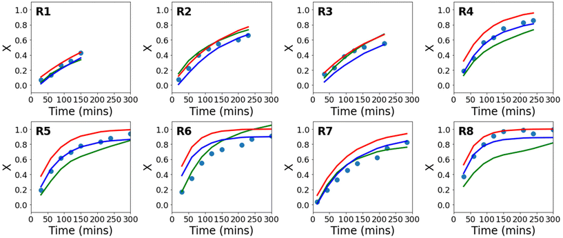 | ||
| Fig. 3 Evolution of conversion with time for experimental data (circles), in comparison to the theoretical evolution of conversion following eqn (16) (red), a conventional neural network (green), and a PCINN (blue). | ||
| Average training error | Average test error | |
|---|---|---|
| Neural network | 0.001 | 0.020 |
| PCINN | 0.003 | 0.006 |
| Eqn (16) | — | 0.021 |
It can be seen from Fig. S3† and Table 3 that the predictive performance of the conventional neural network model in the training set is very good. However, Fig. 3 shows that in the absence of the additional information provided by the gradients (eqn (7)–(9)), performance in the test set is not good and predictions are made that are not physically reasonable. For example, in reaction 6 the predicted final conversion is above 1. Because of the small amounts of experimental data, the training process is also highly variable and leads to significant differences in the final trained network from run to run. This is understandable since looking at the reaction conditions in Table 1, in almost all cases the test reaction is outside of the limits of reaction conditions that it is trained on and therefore the neural network is extrapolating from the small amount of data available. The relatively small dataset used results in severe overfitting and poor predictive performance in the test set.
Looking at Fig. 3 and Table 3 it can also be seen that in terms of absolute error, the first principles solution from eqn (16) using fixed rate coefficients obtained from literature is also relatively poor, even though it is in reasonable agreement with the general trends of the experiments.
For the PCINNs, the incorporation of the derivatives from the underlying chemistry avoids the overfitting seen for the conventional neural network and forces the model towards physically reasonable predictions. As such, the performance in the test set is substantially improved. As the data driven component is incorporated in the PCINN, it also has better predictive performance than the kinetic model as it can account for errors deriving from the differences between model and experimental data.
MMA solution polymerization – prediction of conversion and molecular weight distribution
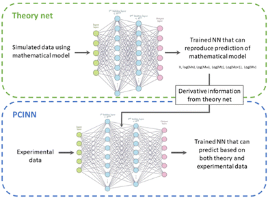
The use of gradients obtained by analytical expressions as described above is unfortunately not feasible for many properties of interest. An example of this is the full molecular weight distribution of the polymer where there is no analytical expression for the derivative with respect to the reaction conditions. In order to overcome this issue, we take the available model that describes the evolution of all species and use it to generate a large amount of training data. This training data is then used to train a neural network that approximates the kinetic model underlying the simulated data. As neural networks are fully differentiable, this allows us to readily generate the approximate gradients of any target parameter, even those for which there is no analytical solution.Thus, our approach, shown schematically in Scheme 3, uses a mathematical model to generate sufficient training data to train a “theory neural network”. This theory neural network is used to provide the gradients to the predictive neural network during the main training stage, which is trained using both experimental data and gradients obtained from the theory network. The output of the network includes predictions of conversion and the averages that define the molecular weight distribution (Mn, Mw, Mz, Mz+1 and Mv). The full molecular weight distribution can then be predicted on the basis of an independently learned neural network trained on simulated data the takes these averages as input and predicts the full molecular weight distribution (see Computational methods section for more information).
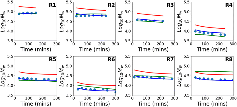
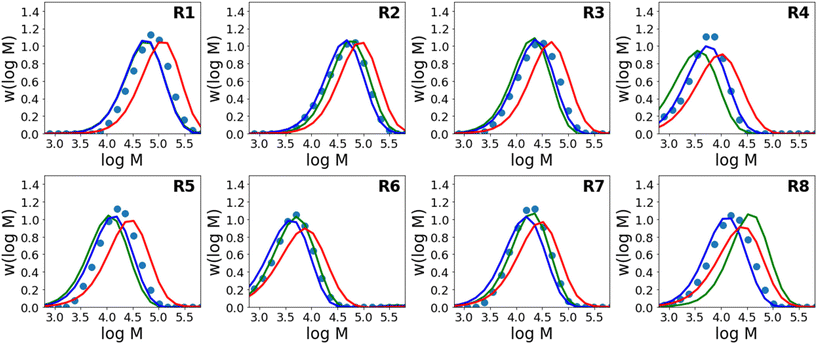
Results for predictions of Mw and the full molecular weight distribution obtained using this approach are shown in Fig. 4 and 5 respectively. Similar to Fig. 3, the results shown are for 8 different models where each model is trained on the data from 7 reactions and tested on 1 reaction. The figure shows only the performance of the test reaction for each of the 8 models.
The results using the data-driven approach alone clearly show that the purely data-driven neural network makes poor predictions which, as discussed above, may be expected due to the relatively limited training set available. Similarly, although the kinetic model is clearly capable of explaining trends in the data, it does not accurately predict the experimental values and results in consistent deviation from the experimental values. These systematic deviations could be related to the use of incorrect rate coefficients, which were taken from the literature without any attempt to fit to the current data, or may alternatively be due to simplifications in the kinetic model, such as the use of a single, chain-length independent value of kt. However, it is remarkable that despite the inability of the kinetic model to describe the data accurately, by combining the data-driven approach and the trends of the kinetic model, a significant improvement in predictive performance can be observed. A summary of the average errors of all the predictive models is shown in Table 4.
| Training error | Test error | |||||
|---|---|---|---|---|---|---|
| X | M n | M w | X | M n | M w | |
| Neural network | 0.001 | 0.001 | 0.000 | 0.026 | 0.043 | 0.025 |
| PCINN | 0.005 | 0.006 | 0.002 | 0.005 | 0.009 | 0.003 |
| Kinetic model | — | — | — | 0.014 | 0.026 | 0.082 |
It is worth mentioning that in the low-data limit, the PCINN approach is expected to result in a network that effectively reproduces the expected trends of the kinetic model. In contrast, the significant overfitting that is seen in the case of the neural network becomes more extreme as the amount of data is further reduced. To exemplify this point, Fig. 6 shows results of trained models using only 1 (R1), 3 (R1–R3), 5 (R1–R5) or 7 (R1–R7) experiments in the training data and tested on reaction 8. It can be seen that the PCINN is able to give reasonable predictions, even with just a single experiment as training data, while the conventional neural network, which is not capable of rational extrapolation, gives poor predictive performance.
On the basis of the low-data predictive capabilities of PCINNs, one potential application is the forecasting of future trajectories of experiments, which would find use in online monitoring and control systems. As opposed to the fixed output of conventional kinetic models, this would allow the system to account for batch-to-batch variations and plant-model discrepancies but would maintain the rationality of first-principles approaches.
To demonstrate this approach, we took as an example reaction 8 and trained a series of models with incoming data measured during the polymerization. Thus, the first model is trained when the first measurement of conversion and molecular weight distribution is obtained and used to predict the future trajectories. As additional datapoints are collected during the experiment, the models are retrained using the all the available data and the predicted trajectories are updated.
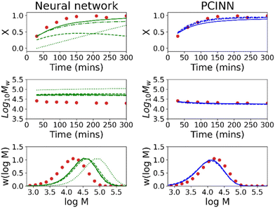
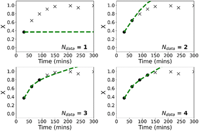
Fig. 7 shows the evolution of predicted trajectories of conversion with increasing number of samples (Ndata) versus the true experimental trajectory for the conventional, purely data-driven neural network. In this case, with a single sample measurement (top left panel) the prediction of future trajectories is understandably poor; the system has no data to learn that conversion increases with time for example. Prediction of future trajectories of molecular weights (see Fig. S4†) are better, but this is largely because the molecular weight does not change significantly during the reaction. As the number of datapoints available increases, predictive performance improves slightly but physically unreasonable estimates are made (i.e. predictions of X > 1) and it was observed that the limited amount of data led to significant run-to-run variability after training. Because the prediction of the full molecular weight distribution requires reasonable estimates of all molecular weight averages, the prediction of the predicted final molecular weight distribution is poor (see Fig. 9).
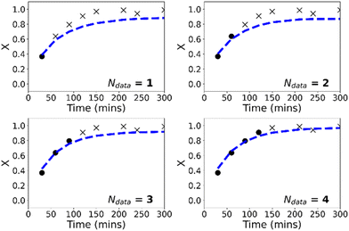
In contrast to the purely data-driven approach, forecasts made by the PCINN models are reasonable from the initial sample for conversion (Fig. 8), for molecular weight (Fig. S5†) and for the full molecular weight distribution (Fig. 9). Unlike the purely data-driven network, the gradients supplied by the theory network provide good estimates of how conversion should evolve with time and ensure that the network is trained to correctly predict expected trends based on first-principles knowledge, even with only a single datapoint for training. As data is fed to the model during the reaction, the network parameters are updated such that the current information is taken into account and the prediction of the future trajectory further improves. As training of the models is rapid (approximately 1 minute on a standard desktop PC) and a single pass through a neural network takes a fraction of a second, this approach would allow the PCINNs to be trained in real-time in response to incoming data to give updated estimates of future trajectories based on a combination of available data and theoretical considerations of the underlying chemistry.
Conclusions
In conclusion, in this work we have discussed a technique for the incorporation of fundamental knowledge of polymerization processes into the training of neural networks to generate predictive models that can perform better than data-driven or conventional mathematical models alone. These Polymer Chemistry Informed Neural Networks (PCINNs) can find practical application in systems where knowledge of the polymerization process is incomplete such that the deviations from theory are compensated by the data-driven component. It may be noted that although the discussion here has focussed on free radical processes, in principle the same techniques can be applied to other polymerization systems, thus opening up possibility for use of PCINNs across a wide spectrum of applications in polymer science.Data availability
The data supporting this article have been included as part of the ESI.† Python source code that shows the implementation of the PCINN is provided at https://github.com/PolymatGIQ/.Conflicts of interest
There are no conflicts to declare.Acknowledgements
The authors would like to acknowledge the funding provided by the Basque Government as part of the IKUR program.Notes and references
- J. M. Asua, J. Polym. Sci., Part A: Polym. Chem., 2004, 42, 1025–1041 CrossRef CAS.
- J. M. Asua, in Polymer Reaction Engineering, John Wiley & Sons, Ltd, 2007, pp. 1–28 Search PubMed.
- T. Meyer and J. T. F. Keurentjes, in Handbook of Polymer Reaction Engineering, 2005, pp. 1–15 Search PubMed.
- P. D. Iedema and N. H. Kolhapure, in Handbook of Polymer Reaction Engineering, 2005, pp. 431–532 Search PubMed.
- M. Wulkow, Macromol. React. Eng., 2008, 2, 461–494 CrossRef CAS.
- A. E. Hamielec and J. B. P. Soares, Prog. Polym. Sci., 1996, 21, 651–706 CrossRef CAS.
- P. Liu, J. Du, Y. Ma, Q. Wang, K. H. Lim and B.-G. Li, Chin. J. Chem. Eng., 2022, 50, 3–11 CrossRef CAS.
- J. M. M. Faust, S. Hamzehlou, J. R. Leiza, J. M. Asua, A. Mhamdi and A. Mitsos, Chem. Eng. J., 2021, 414, 128808 CrossRef CAS.
- M. Vicente, S. Benamor, L. M. Gugliotta, J. R. Leiza and J. M. Asua, Ind. Eng. Chem. Res., 2001, 40, 218–227 CrossRef CAS.
- M. Vicente, C. Sayer, J. R. Leiza, G. Arzamendi, E. L. Lima, J. C. Pinto and J. M. Asua, Chem. Eng. J., 2002, 85, 339–349 CrossRef CAS.
- D. R. D′hooge, P. H. M. Van Steenberge, M.-F. Reyniers and G. B. Marin, Prog. Polym. Sci., 2016, 58, 59–89 CrossRef.
- J. Fiosina, P. Sievers, M. Drache and S. Beuermann, Comput. Chem. Eng., 2023, 177, 108356 CrossRef CAS.
- J. Fiosina, P. Sievers, M. Drache and S. Beuermann, ACS Polym. Au, 2024, 4, 438–448 CrossRef CAS PubMed.
- N. B. Ishola and T. F. L. McKenna, Can. J. Chem. Eng., 2024, 102, 2228–2243 CrossRef CAS.
- N. B. Ishola and T. F. L. McKenna, Macromol. Theory Simul., 2021, 30, 2100059 CrossRef CAS.
- I. Goodfellow, Y. Bengio and A. Courville, Deep Learning, MIT Press, 2016 Search PubMed.
- T. B. Martin and D. J. Audus, ACS Polym. Au, 2023, 3, 239–258 CrossRef CAS PubMed.
- C. Kuenneth and R. Ramprasad, Nat. Commun., 2023, 14, 4099 CrossRef CAS PubMed.
- H. D. Tran, C. Kim, L. Chen, A. Chandrasekaran, R. Batra, S. Venkatram, D. Kamal, J. P. Lightstone, R. Gurnani, P. Shetty, M. Ramprasad, J. Laws, M. Shelton and R. Ramprasad, J. Appl. Phys., 2020, 128, 171104 CrossRef.
- K. Farajzadehahary, X. Telleria-Allika, J. M. Asua and N. Ballard, Polym. Chem., 2023, 14, 2779–2787 RSC.
- L. Tao, V. Varshney and Y. Li, J. Chem. Inf. Model., 2021, 61, 5395–5413 CrossRef CAS PubMed.
- G. Cybenko, Math. Control. Signals Syst., 1989, 2, 303–314 CrossRef.
- S. Thrun, in Explanation-Based Neural Network Learning: A Lifelong Learning Approach, Springer, US, Boston, MA, 1996, pp. 19–48 Search PubMed.
- T. M. Mitchell and S. B. Thrun, in Advances in Neural Information Processing Systems, ed. S. Hanson, J. Cowan and C. Giles, Morgan-Kaufmann, 1992, vol. 5 Search PubMed.
- P. Simard, B. Victorri, Y. LeCun and J. Denker, in Advances in Neural Information Processing Systems, ed. J. Moody, S. Hanson and R. P. Lippmann, Morgan-Kaufmann, 1991, vol. 4 Search PubMed.
- G. E. Karniadakis, I. G. Kevrekidis, L. Lu, P. Perdikaris, S. Wang and L. Yang, Nat. Rev. Phys., 2021, 3, 422–440 CrossRef.
- M. Raissi, P. Perdikaris and G. E. Karniadakis, J. Comput. Phys., 2019, 378, 686–707 CrossRef.
- D. Kukulj, T. P. Davis and R. G. Gilbert, Macromolecules, 1998, 31, 994–999 CrossRef CAS.
- A. Butté, G. Storti and M. Morbidelli, Macromol. Theory Simul., 2002, 11, 22–36 CrossRef.
- S. Kumar and D. Ramkrishna, Chem. Eng. Sci., 1996, 51, 1311–1332 CrossRef CAS.
- Initiators for high polymers – Akzo Nobel, 2006.
- D. S. Achilias and C. Kiparissides, Macromolecules, 1992, 25, 3739–3750 CrossRef CAS.
- S. Beuermann, M. Buback, T. P. Davis, R. G. Gilbert, R. A. Hutchinson, O. F. Olaj, G. T. Russell, J. Schweer and A. M. van Herk, Macromol. Chem. Phys., 1997, 198, 1545–1560 CrossRef CAS.
- W. Wang and R. A. Hutchinson, AIChE J., 2011, 57, 227–238 CrossRef CAS.
- Y. Nakamura and S. Yamago, Macromolecules, 2015, 48, 6450–6456 CrossRef CAS.
- A. Paszke, S. Gross, F. Massa, A. Lerer, J. Bradbury, G. Chanan, T. Killeen, Z. Lin, N. Gimelshein, L. Antiga, A. Desmaison, A. Köpf, E. Z. Yang, Z. DeVito, M. Raison, A. Tejani, S. Chilamkurthy, B. Steiner, L. Fang, J. Bai and S. Chintala, CoRR, 2019 DOI:10.48550/arXiv.1912.01703.
Footnotes |
| † Electronic supplementary information (ESI) available. See DOI: https://doi.org/10.1039/d4py00995a |
| ‡ Although the partial derivative with respect to temperature is available in an analytical form, the resulting expression is not reproduced here due to the length of the resulting equation. |
| This journal is © The Royal Society of Chemistry 2024 |

