Application of PLS–NN model based on mid-infrared spectroscopy in the origin identification of Cornus officinalis

Abstract

Mid-infrared spectroscopy has been increasingly used as a nondestructive analytical technique in Chinese herbal medicine identification in recent years. In this study, a new chemometric model named as PLS–NN model was proposed based on the mid-infrared spectral data of Cornus officinalis samples from 11 origins. It was realized by combining the partial least squares and neural networks for the identification of the origin of Chinese herbal medicines. First, we extracted features from the spectral data in 3448 bands using the partial least squares method, and extracted 122 components that contained more than 95% of the information. Then, we trained the PLS–NN model by neural network using the extracted components as inputs and the corresponding origin classes as outputs. Finally, based on an external test set, we evaluated the generalization ability of the PLS–NN model using metrics such as accuracy, F₁-Score and Kappa coefficient. The results show that the PLS–NN model performs well in all three metrics when compared to models such as Decision trees, Support vector machine, Partial least squares Discriminant analysis, and Naive bayes. The model not only realizes the dimensionality reduction of full-spectrum data and improves the training efficiency of the model, but also has higher accuracy compared with the full-spectrum data model. The PLS–NN model was applied to identify the origin of Cornus officinalis with an accuracy of 91.9%.

---

1. Introduction

China is geographically and climatically very favorable for the growth of herbal medicines, which has resulted in many Chinese-grown herbal medicines enjoying a good reputation both at home and abroad and being exported to many regions and countries.¹ Compared with synthetic drugs, herbal medicines have the advantages of stable efficacy, low toxicity and side effects, adaptability to individual differences and natural raw materials, which has made more and more regions and countries begin to pay attention to the value of herbal medicines.^2–4 However, with the gradual deterioration of the natural ecological environment, the growing environment of wild Chinese herbal medicines has been damaged, and the supply of some wild Chinese herbal medicines is in short supply, leading to confusion in the market of Chinese herbal medicines. In addition, there is a wide variety of traditional Chinese medicinal materials, and different regions have different medicinal practices. The common occurrence of homonyms, synonymous names, and mixed varieties makes authenticating traditional Chinese medicines a challenge.^5,6

Traditional herbal medicine identification methods include appearance identification, physical and chemical properties identification and microscopic identification.^7,8 Appearance identification is mainly carried out by observing the external form, color, smell and other characteristics of herbs. This method is simple and easy to implement, and is applicable to some herbs with obvious appearance characteristics, but it does not have high accuracy for herbs with similar appearance.^9,10 Physical and chemical property identification is carried out by testing the physical and chemical properties of herbs, such as solubility, melting point and specific gravity. This method relies on the physicochemical characteristics of the herbs and can provide some basis for qualitative identification, but is limited for quantitative and specific identification. Microscopic identification is carried out by microscopic observation of the cellular structure, tissue structure and other characteristics of the herbal medicine. This method can provide more detailed morphological information and has a certain degree of accuracy for the identification of specific herbs.¹¹ However, microscopic identification mainly relies on morphological and anatomical features of herbs, and it is difficult to draw quantitative conclusions about the quality of herbs, and the method can only be used for auxiliary identification, but not for quality evaluation alone.

With the continuous progress of science and technology, the application of modern chromatographic coupling techniques has led to a significant improvement in the efficiency and accuracy of the detection of herbal medicines. Chromatographic techniques commonly used for the identification of herbal medicines include high performance liquid chromatography,^12,13 capillary gas chromatography,^14,15 thin-layer chromatography^16,17 and liquid chromatography-mass spectrometry.^18,19 The advantages of these methods are the qualitative and quantitative analysis of the chemical constituents of herbal medicines with excellent characteristics such as accuracy, sensitivity, rapidity and good reproducibility at the same time, which can provide a scientific basis for the quality control and safe use of herbal medicines. However, chromatographic techniques also have some shortcomings in the identification of herbal medicines, such as high requirements for instrumentation, complex analytical methods and difficulties in sample preparation.^20–22

Infrared spectroscopy stands as a commonly utilized method for the identification and characterization of chemical substances. It has a wide range of applications in the field of herbal medicine identification and continues to make progress with the development of technology.^23,24 Infrared spectroscopic identification is based on the principle of using the vibration and rotation of molecules in a specific frequency range to produce a characteristic spectral image by absorbing, scattering or transmitting light. These spectra can be used to identify and quantitatively analyze the chemical constituents in the sample. The use of infrared spectroscopy to realize the identification of Chinese herbal medicines has the advantages of high efficiency, non-destructiveness and reliability. Yang et al. successfully identified Bupleuri Radix based on geographic origin by using Principal Component Analysis (PCA), Partial Least Squares Discriminant Analysis (PLS-DA), and Support Vector Machine (SVM) based on near-infrared spectra.²⁵ Using mid-infrared spectroscopy in combination with chemometrics, Guo et al. developed a quantitative method to assess the quality of danshen granules. The results of the study showed that Fourier transform mid-infrared spectroscopy combined with Partial Least Squares (PLS) regression is a rapid and valuable analytical tool to accurately determine the water-soluble extract of single yinpian in danshen granules based on excipient content.²⁶ Jin et al. used PCA to dimensionalize the Cornus officinalis spectral data, and then realized the identification of Cornus officinalis origin using SVM, and the results indicated that the accuracy of this combined model was 84.8%.²⁷

Cornus officinalis is the dried mature fruit pulp of Cornus officinalis, a plant in the Cornaceae family.²⁸ It has the effects of tonifying the liver and kidneys, astringent and astringent, in addition to its cardiotonic, anti-inflammatory, antibacterial, anti-stress, antioxidant and hypolipidemic effects. Cornus officinalis is native to China and is mainly found in the northern and southwestern parts of the country. In addition, Cornus officinalis is also distributed in some other Asian countries such as Mongolia, North Korea and South Korea. We collected mid-infrared spectral data of Cornus officinalis from a total of 11 origins (OP 1–OP 11) in Zhejiang, Anhui, Jiangxi, Shandong, Henan, Hunan, Sichuan, Shaanxi, and Gansu for identification modeling. PLS was used to implement dimensionality reduction on full-spectrum data and combined with Neural Networks (NN) to model the identification of Cornus officinalis origin. In this paper, we refer to this PLS combined NN model as the PLS–NN model. Comparison with other common classification discriminant models such as Decision trees, SVM, PLS-DA, and Naive bayes model reveals that our model performs excellently in some common evaluation metrics such as accuracy, F-Score, and Kappa coefficient.^29–31 The model not only provides an accurate nondestructive method for the rapid identification of the origin of Cornus officinalis, but also can be extended to the identification of other Chinese herbs, which is of positive significance for the control of the quality of traditional Chinese medicine and the promotion of the development of the traditional Chinese medicine industry.

2. Material and methods

2.1. Data source and preprocessing

The spectral characteristics of different herbs vary greatly. Even for the same herb from different places of origin, they will exhibit distinct spectral features under near-infrared and mid-infrared irradiation, primarily due to differences in the chemical composition of inorganic elements and organic substances. Therefore, these features can be effectively utilized for the identification of Chinese herbal medicines in terms of their types and origins.

In this study, a set of spectral data of Cornus officinalis measured by Chengdu University of Traditional Chinese Medicine was collected with the aim of constructing an origin identification model for Chinese herbal medicines (https://www.mcm.edu.cn/html_cn/node/90d223833c1eb50f899aa096a66c6896.html). The dataset contained 658 samples of Cornus officinalis from 11 different origins. Each sample was subjected to infrared spectroscopy measurements in the wavenumber range of 551–3998 cm⁻¹, and their absorbance was recorded.

Before the sample data can be analyzed, the collected data needs to be preprocessed. The outlier detection method based on interquartile range was used in the study to identify data greater than 1.5 times the sum of the left and right nearest neighbor values as outliers. For outliers and missing values, we used the moving average interpolation method for data processing. Considering the wide range of spectral wave numbers and the limitations of sample measurement accuracy, no special treatment would be given to duplicate values in the data. The mid-infrared spectral data processed by the moving average interpolation method were summarized, and the summarized absorbance range was −0.007–1.487 AU. It should be noted that 626 sets of data in the last 184 bands have negative absorbance values, which is due to the fact that the absorbance data collected are instrumentally corrected values. Since these negative values are small in absolute value and do not exceed 0.001% of the total data, they are not treated specifically. There are 31 141 data in the sample with absorbance greater than 1 AU, accounting for 1.373% of the total. However, the maximum value of absorbance did not exceed 1.5 AU, and did not deviate from the Lambert–Beer law, so it was not treated specifically in this study.

2.2. PLS–NN model construction process

The core of the PLS–NN model is to combine the PLS and NN models to realize the dimensionality reduction and origin identification of the spectral data. Fig. 1 demonstrates its specific flow. The processed dataset is first randomly divided into training set and test set.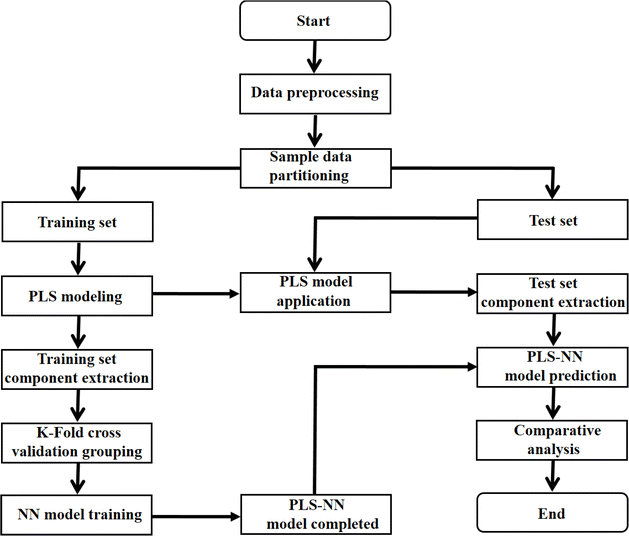

Fig. 1 The flow chart of PLS–NN model based on the mid-infrared spectral data of Cornus officinalis and K-fold cross validation.

In the training set, PLS regression was utilized for modeling. PLS regression amalgamates the benefits of multiple linear regression, PCA and canonical correlation analysis. By addressing the correlation among parameters, it effectively mitigates multicollinearity issues within variables.^32,33 For modeling problems involving p dependent variables and m independent variables, PLS regression is employed to examine the statistical relationships among them. Given the observed n sample points, data tables X and Y containing the independent and dependent variables are compiled. In this context, PLS regression initially extracts t and u from X and Y, respectively, aiming to capture as much information as possible regarding the variances in their respective data tables and to maximize their correlation. After the first component has been extracted, PLS regression is implemented for X versus t and Y versus t, respectively. The algorithm terminates if the regression equation has reached a satisfactory accuracy, otherwise, a second round of component extraction is performed using the residual information after X has been interpreted by t as well as the residual information after Y has been interpreted by t. This is repeated until a more satisfactory accuracy can be achieved.³⁴

The selection of the number of components needs to be completed next to obtain a regression model with good predictive power. For the number l of principal components to be extracted for modeling, it can be determined by a cross validity test. The i-th observation is removed each time and the remaining n − 1 observations are used to model the regression by PLS regression. The fitted regression equation after extracting the h components is considered in the modeling process. Substituting the removed i-th observation into the fitted regression equation obtains the predicted value yŷ_(i)j(h) of y_j(j = 1,2,⋯,p) at the i-th observation. Repeat the above validation for i = 1,2,⋯,n to obtain the predicted residual sum of squares for the j-th dependent variable y_j(j = 1,2,⋯,p) at the time of extracting h components (eqn (1)). Eqn (2) is the predicted residual sum of squares of y_j(j = 1,2,⋯,p), when PRESS(h) reaches the minimum value, the corresponding h is the number of extracted components.

With the PLS model constructed on the training set, we successfully extracted the components from both the training and test sets. These extracted components not only preserve crucial information but also eliminate redundant data, thereby providing high-quality inputs for the subsequent training of the NN model. Subsequently, utilizing the extracted training set components as inputs, we proceeded to construct the NN architecture and train it.

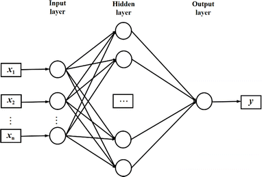
NN is a machine learning model used to solve classification problems. Fig. 2 shows its architecture. It consists of multiple layers, which include an input layer, hidden layers, and an output layer. Each hidden layer consists of multiple neurons (also referred to as the size of each layer) that are connected to all the neurons in the previous layer through connection weights. In a NN, each neuron receives inputs from the previous layer and applies an activation function to nonlinearly transform the inputs. RELU(x),tanh(x) and σ(x) (eqn (3)–(5)) are the commonly used activation functions. The number of neurons in the hidden layer determines the complexity of the features that the model can learn, while the number of hidden layers determines the depth and expressiveness of the model.^35,36

Fig. 2 The architecture of the neural network.

In the training process of the NN, we utilized K-fold cross validation to partition the training set and employed the cross-entropy loss function to quantify the difference between model predictions and true labels. Eqn (6) is the cross-entropy loss function, where y is the true label vector, yŷ is the predicted output vector of the NN, and p is the number of classes. The connection weights are continuously adjusted by the optimization algorithm to minimize the loss function, so as to train a PLS–NN model with good performance. Finally, the model is applied to the components of the test set to complete the prediction of the test set, and the results are compared and analyzed, in order to test the performance and generalization ability of the model.

3. Establishment of origin identification model

3.1. Data exploratory analysis

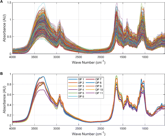
Exploratory analysis of the data was highly beneficial in gaining initial insight into the relationship between spectral information and origin. We plotted the spectral data for all Cornus officinalis samples in Fig. 3. It can be seen that the infrared spectral data are similar in 658 groups of Cornus officinalis, which is due to the fact that different kinds of herbs usually contain similar basic chemical constituents and functional groups. These common chemical compositions and functional groups can lead them to exhibit similar features in the infrared spectrum.

Fig. 3 (A) Mid-infrared spectrograms of 658 samples of Cornus officinalis from 11 different origins; (B) comparison of average mid-infrared spectra of Cornus officinalis samples from 11 different origins. Figures are generated using Matlab (Version R2023a, https://www.mathworks.com/) [Software].

The spectral data showed high absorbance in the intervals 3600–2800 cm⁻¹ and 1800–1000 cm⁻¹ with typical valleys and peaks. The hydroxyl functional group in Cornus officinalis exhibits a broad absorption peak appearing at 3600–3200 cm⁻¹, and this peak can be used for the detection of the content of active ingredients in Cornus officinalis. The characteristic peaks located in the range 3000–2900 cm⁻¹ represent the stretching vibrations of the aliphatic alkyl group. The ketone group functional group appeared at 1700–1750 cm⁻¹, which showed a sharp absorption peak, and the wave number corresponding to this peak can be used to determine the presence of ketones in Cornus officinalis. The characteristic peak near 1400 cm⁻¹ is the aromatic ring backbone vibration absorption peak. There is a characteristic peak in the interval 1200–1000 cm⁻¹ representing the stretching vibration of glycogen. It can be intuitively seen that in some bands, such as 3400–3200 cm⁻¹ and 1700–1550 cm⁻¹ bands, there are some differences in the spectral data of different origins. This is due to the fact that Cornus officinalis from different origins is affected by the growing environment, soil, climate and other environmental factors, resulting in differences in its chemical composition, which in turn presents differences in the infrared spectral data.

The spectral differences reflect the differences in the composition of Chinese herbal medicine samples, which can be visually expressed by the degree of overlap of spectral lines in the overlapping spectral graphs. These intuitive differences can be quantitatively expressed by the Euclidean distance between spectral vectors, the cosine of the included angle, and the Pearson linear correlation coefficient. In this paper, the Pearson linear correlation coefficient (eqn (7)) is used to describe the spectral differences of Chinese herbal medicines from different origins.

Table 1 shows the correlation coefficients between the spectral vectors of 11 different origins of Cornus officinalis. It can be seen that the cornelian cherry spectra of OP 7 and OP 11 have the highest similarity with correlation coefficients as high as 0.999. This indicates that the composition of the Cornus officinalis samples from the two origins is very similar, which is related to the similar climatic and geographic conditions of the two origins. The identification of these two origins by spectral analysis is the most difficult. The lowest spectral similarity was found between Cornus officinalis from OP 5 and OP 8, with a correlation coefficient of 0.982, which suggests that there are differences in the composition of Cornus officinalis samples from these two origins. It is easier to identify the Cornus officinalis from these two origins by spectral analysis. The spectral similarity of all Cornus officinalis samples between the origins exceeded 0.98 and passed the correlation test at the 0.01 level of significance, indicating that the spectral vectors of the same type of herbs are significantly correlated.

Table 1 The Pearson linear correlation coefficients between the spectral vectors of Cornus officinalis from 11 different origins (band ** indicates significant correlation at a significant level of 0.01)

OP	OP 1	OP 2	OP 3	OP 4	OP 5	OP 6	OP 7	OP 8	OP 9	OP 10	OP 11
OP 1	1.000	0.996**	0.998**	0.990**	0.986**	0.997**	0.996**	0.997**	0.989**	0.990**	0.998**
OP 2		1.000	0.995**	0.995**	0.989**	0.997**	0.998**	0.997**	0.992**	0.994**	0.998**
OP 3			1.000	0.990**	0.985**	0.997**	0.996**	0.995**	0.991**	0.991**	0.997**
OP 4				1.000	0.998**	0.995**	0.996**	0.990**	0.998**	0.996**	0.996**
OP 5					1.000	0.992**	0.990**	0.982**	0.998**	0.996**	0.992**
OP 6						1.000	0.998**	0.995**	0.995**	0.993**	0.998**
OP 7							1.000	0.998**	0.994**	0.991**	0.999**
OP 8								1.000	0.986**	0.985**	0.996**
OP 9									1.000	0.997**	0.995**
OP 10										1.000	0.995**
OP 11											1.000

---

3.2. Mid-infrared spectral feature extraction

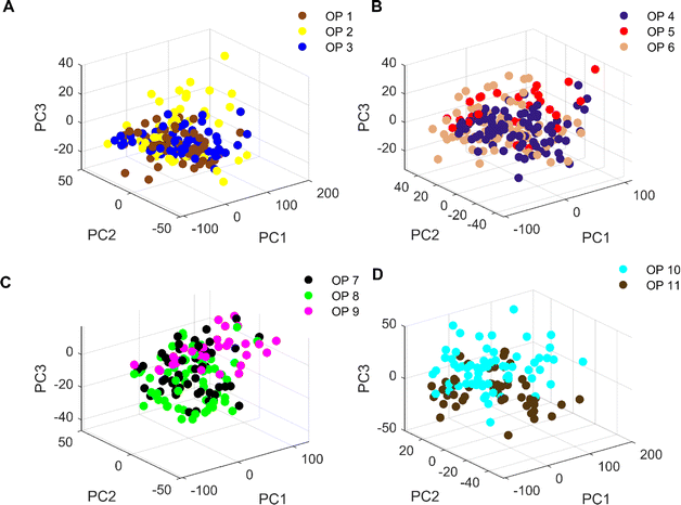
The spectral vectors of the same type of herbs are similar, so in order to effectively identify and differentiate the same herbs from different origins, further chemometric modeling is required. PCA was used to analyze the mid-infrared spectral ensembles of Cornus officinalis samples from different origins before constructing the model in order to visualize the differences of Cornus officinalis samples from different origins. As can be seen from Fig. 4, the first three eigenvalues of the mid-infrared spectral matrix are 2755, 314.31 and 174.91, respectively. The cumulative contribution rates of the first three eigenvalues are 80.8%, 89.9% and 95%, respectively, indicating that the first three eigenvalues can adequately represent the collected spectral matrix.³⁷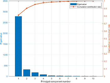

Fig. 4 The principal component eigenvalues and the cumulative contribution rate of the spectral data.

Fig. 5 shows the 3D plot of principal component scores constructed from the first 3 eigenvalues of the spectral matrix. It should be noted that due to the large number of origins of Cornus officinalis, samples of Cornus officinalis from 11 origins were categorized into 3, 3, 3 and 2 different categorical groups according to their quantities for comparison and analysis. We can see that only the samples of Cornus officinalis from OP 1 and OP 3 are relatively concentrated, while the samples from other origins are relatively scattered. In addition, among the samples of various origins, there are large crossings and overlaps between them, and the boundaries between the samples are not clear enough. This suggests that the differences between samples of Cornus officinalis from various origins are not so obvious that they cannot be effectively distinguished by PCA. Therefore, we need to further resort to chemometric methods to realize the identification of samples from different origins.

Fig. 5 (A) Distribution of three-dimensional principal component scores of Cornus officinalis samples from OP 1–OP 3; (B) distribution of three-dimensional principal component scores of Cornus officinalis samples from OP 4–OP 6; (C) distribution of three-dimensional principal component scores of Cornus officinalis samples from OP 7–OP 9; (D) distribution of three-dimensional principal component scores of OP 10 and OP 11 Cornus officinalis samples.

The mid-infrared spectral data of Cornus officinalis from different origins were divided into the training set and the test set according to the ratio of 7 : 3. The spectral data were divided by overall random partitioning, i.e., the 658 samples were regarded as a whole, and then the samples were randomly assigned according to a predetermined ratio. The training set was used to establish the Cornus officinalis origin recognition model, and the test set was used to test the identification effect of the model. Unbalanced samples affect the robustness and generalization ability of the model and may lead to bias, underfitting, or overfitting. Following the principle of balanced sample size leads to a more accurate, robust and better generalized model. The balance of the samples needs to be discussed as there were a total of 11 origins of Cornus officinalis samples in this study and the number of samples from each origin was different. As can be seen from Fig. 6, in the training set, the maximum number of samples from OP 6 is 65, and the minimum number of samples from OP 5 is 21. In the test set, the maximum number of samples from OP 1 is 30, and the minimum number of samples from OP 5 is 8. In the all sets, the maximum number of samples from OP 4 is 88, and the minimum number of samples from OP 5 is 29. The ratio of the maximum number of samples from different origins to the minimum number of samples, whether in the training set, the test set, or all sets, does not exceed 4 : 1, so we consider that the model does not have a sample imbalance, and that no classification weights is needed in the model training process.

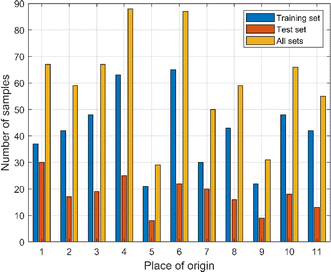Fig. 6 The number of samples in the training set, test set and all sets of Cornus officinalis from different origins.

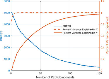
The number of variables in the full-spectrum data is large and the spectral vectors are highly correlated with each other. Directly inputting all variables into the origin identification model would increase the computational complexity and may lead to multicollinearity in the model, thus reducing the generalization ability of the model and increasing the risk of overfitting. Both PCA and PLS are commonly used methods for solving multicollinearity problems in full-spectrum data. PCA is a simple and intuitive linear transformation method that is easy to understand and implement. However, it only considers the variance of the independent variables and not the dependent variable. In contrast, PLS is a supervised learning method that is able to consider the relationship between the independent and dependent variables simultaneously. In addition, PLS tends to show excellent performance in small sample datasets. Therefore, PLS is chosen in this study to reduce the dimensionality of the full-spectrum data and to deal with the multicollinearity problem in it. Fig. 7 shows the plot of the number of PLS components versus the PRESS distribution and Percent Variance Explained. It can be seen that the PRESS value tends to decrease with the increase of the PLS component, and when the PLS component exceeds 120, the continued increase of the component has almost no effect on the PRESS. At a PLS component of 122, the corresponding PRESS value is 439.55. Meanwhile, the percentage of variance explained by X is 100% and the percentage of variance explained by Y is 95.07%, i.e., what percentage of the total variance explained by these PLS components is more than 95% for both the independent and dependent variables. These results indicate that we can choose 122 as the number of components in constructing the origin identification model of Cornus officinalis samples.

Fig. 7 The plot of the number of PLS components versus the PRESS distribution and percent variance explained, where the horizontal axis represents the number of PLS components, the left vertical axis represents PRESS, and the right vertical axis represents percent variance explained.

3.3. PLS–NN model construction

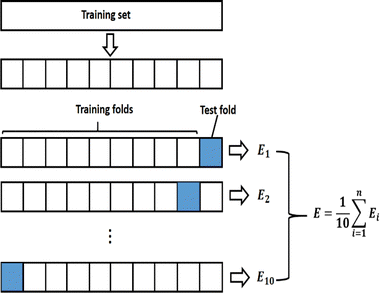
NN are powerful nonlinear models that are adept at handling complex classification tasks by capturing complex patterns in data. In this study, a Cornus officinalis origin identification model was established using NN based on the optimal number of PLS components of Cornus officinalis infrared spectral data. The spectral components extracted by PLS in the training set were used as predictor variables, and Cornus officinalis origin was used as response variable to build the model with the help of NN classifier in Matlab 2023a.

Overfitting occurs when a model excels on training data but falters on novel data. To address this in NN classifiers, K-Fold cross-validation is employed. In this technique, the dataset is randomly partitioned into K mutually exclusive subsets. The model is trained K times, utilizing K-1 subsets for training and the remaining one for validation in each iteration. This generates K models, each validated once. The average performance metrics across these models serve as the final evaluation, as depicted in Fig. 8. This technique fully utilizes all the samples in the dataset for training and validation, reducing the impact of dataset partitioning on the training results. Since the number of samples included in the training set is 461, in order to achieve a more reliable performance evaluation of the model and to reduce the bias that may be induced by the limited number of samples, in this study K is selected as 10.

Fig. 8 10-fold cross-validation process description and implementation.

Accuracy is one of the most common metrics for evaluating classification models. It indicates the proportion of samples that the model predicts correctly out of the total number of samples. The higher the accuracy, the better the performance of the model. Eqn (8) is an expression for accuracy, where TP is true positives, which means the number of samples that the model correctly predicts as positive cases, FN is false negatives, which means the number of samples that the model incorrectly predicts as negative cases, FP is false positives, which means the number of samples that the model incorrectly predicts as positive cases, and TN is true negatives, which means the number of samples that the model correctly predicts as negative cases.

In constructing the NN model, the data was first normalized to eliminate the scale difference between different features and enhance the performance and stability of the model. Then the selection of hyperparameters was carried out, which includes the number of fully connected layers, first layer size, second layer size, third layer size, activation functions and regularization strength. In practice, for simple problems, shallower NN are usually used, and the number of fully connected layers is usually between 1–3. For the size of each layer, we set it at [1300] for optimization. ReLU, Tanh and σ are commonly used activation functions and we search between all three of them. For regularization strength, we use the default L2 norm regularization and set the search range to , where n is the number of observations.

Bayesian optimizer is a commonly used optimization method that has been widely applied to hyperparameter tuning. It not only reduces the time and effort of manual parameter tuning, but also improves the performance of the model. In this study, we set the acquisition function in the Bayesian optimizer to the software's default expected improvement per second plus and set the number of iterations to 30 in order to optimize the search for the hyperparameters of the NN model. With the help of Bayesian optimizer, the optimal number of fully connected layers, first layer size, second layer size, third layer size, activation functions, regularization strength are determined as 3, 206, 31, 27, Tanh and 5.41 × 10⁻⁵, respectively. At this point, the accuracy of the NN model in the validation set reaches 100%. It shows that the model has a good performance in the training set. With the help of Matlab software, the PLS–NN model of Cornus officinalis origin identification was completed.

The PLS–NN model achieved good performance in the training set of Cornus officinalis samples, but the performance in the test set was more important. The 197 test samples were input into the trained PLS–NN model to compare the predicted results with the true results. The confusion matrix is a tool commonly used to evaluate classification model performance, showing the relationship between predicted and true results in a tabular format. Each column represents true results, each row represents predicted results. Precision (eqn (9)) and recall (also called Sensitivity, eqn (10)) are displayed on the rightmost side of rows and bottom of columns, respectively, with accuracy at the bottom right corner.³⁸

It can be seen from Fig. 9 that all samples of Cornus officinalis predicted to be OP 1, OP 2, OP 10 and OP 11 were from the corresponding origins, all with 100% precision. Of the 27 samples predicted to be OP 7, only 19 are from OP 7, which has the lowest precision of 70.4%. In addition, all samples of Cornus officinalis from five origins, OP 3, OP 4, OP 5, OP 6 and OP 11, were identified by the model with 100% recall. Only 13 of the 18 samples from OP 10 were identified by the model, and it had the lowest recall of 72.2%. There were 4 samples from OP 10 that were incorrectly predicted as OP 7 by the model, which indicates that there is some difficulty in identifying between OP 10 and OP 7 using the PLS–NN model. Overall, 181 out of 197 samples were correctly predicted with an accuracy of 91.9%. This maintains the same high accurate as the validation set, indicating that the PLS–NN model has a strong generalization ability and can effectively achieve the identification of the origin of Cornus officinalis samples.

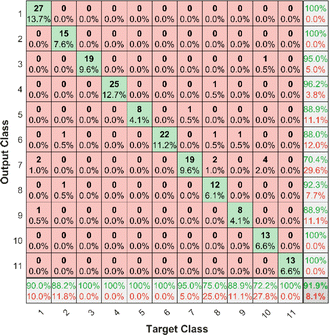Fig. 9 Confusion matrix for Cornus officinalis test samples. Each column of the confusion matrix represents the true origin, and each row represents the predicted origin.

4. Discussion

The quality and efficacy of Chinese herbal medicines are often closely related to their origin, so rapid and accurate identification of the origin of Chinese herbal medicines is of great practical significance. Based on the mid-infrared spectral data, the PLS–NN model can effectively realize the identification of the origin of Cornus officinalis. In addition, Decision trees, SVM, PLS-DA, Naive bayes and full-spectrum NN models can be implemented to identify the origin of Cornus officinalis.

In order to make a quantitative comparison of the individual models, we trained these models using the same training set and compared the results of the test set to the PLS–NN model. During model training, we still used 10-fold cross-validation and optimized the hyperparameters of each model with the help of the default Bayesian optimization in the classification learner. In the Decision trees, the maximum number of splits was chosen to be 92 and the splitting criterion was chosen to be the maximum deviation reduction. In the SVM model, the kernel function was chosen to be a Gaussian kernel, the kernel scale was chosen to be 11, the box constraint level was chosen to be 1, and the multiclass method was chosen to be one-vs.-one. In the PLS-DA model, the covariance structure was chosen as diagonal covariance structure. In the Naive bayes model, the kernel type was selected as Gaussian and the support option was selected as unbounded. In the full-spectrum NN model, the optimal number of fully connected layers, first layer size, second layer size, third layer size, activation functions, regularization strength were determined as 3, 199, 33, 25, Tanh and 4.81 × 10⁻⁵, respectively.

Based on the results in Table 2, we can observe that in terms of precision: the SVM model achieves 100% precision in 9 origins but less than 60% in OP 6 and OP 10; the PLS-DA model achieves 100% precision in 5 origins but only 30% in OP 10; the Naive bayes model achieves 100% precision in 3 origins but less than 40% in OP 5 and OP 10; and the PLS–NN model achieves 100% precision in 4 origins and is more than 70% precise in all 11 origins. In terms of recall, in OP 8 and OP 9, the NN model has the highest recall, which is 81.2% and 100%, respectively. In OP 10, the SVM model, the PLS-DA model and the NN model have the highest recall, all at 100%. The PLS–NN model has the highest recall for all but these three origins, and it has more than 70% recall for all 11 origins.

Table 2 Precision and Recall (sensitivity) of each Cornus officinalis origin identification model in 11 different origins, where PPV stands for precision and TPR stands for sensitivity (values are measured in %)

OP	Decision trees		SVM		PLS-DA		Naive bayes		NN		PLS–NN
	PPV	TPR	PPV	TPR	PPV	TPR	PPV	TPR	PPV	TPR	PPV	TPR
OP 1	92.3	40.0	100	46.7	100	53.3	93.8	50.0	100	83.3	100	90.0
OP 2	44.4	70.6	100	70.6	100	64.7	81.2	76.5	87.5	82.4	100	88.2
OP 3	57.1	63.2	100	84.2	93.3	73.7	100	68.4	73.9	89.5	95.0	100
OP 4	70.0	84.0	100	96.0	100	84.0	100	84.0	96.2	100	96.2	100
OP 5	60.0	75.0	100	62.5	87.5	87.5	38.5	62.5	88.9	100	88.9	100
OP 6	52.2	54.5	58.8	90.9	72.2	59.1	56.0	63.6	81.5	100	88.0	100
OP 7	66.7	50.0	100	75.0	94.7	90.0	84.6	55.0	85.7	60.0	70.4	95.0
OP 8	52.9	56.2	100	56.2	100	62.5	90.0	56.2	81.2	81.2	92.3	75.0
OP 9	66.7	66.7	100	33.3	100	55.6	100	44.4	100	100	88.9	88.9
OP 10	47.1	44.4	34.6	100	30.0	100	29.6	88.9	100	100	100	72.2
OP 11	46.7	53.8	100	100	85.7	92.3	91.7	84.6	85.7	92.3	100	100

---

The F₁-Score is a measure of the performance of a classification model, which is the harmonic mean of Precision and Recall. The F₁-Score ranges from 0 to 1, and the closer it is to 1, the better the performance of the classification model. In multicategorization problems, if the F₁-Score of the model is to be calculated, there are two ways of calculating it, Micro-F₁ and Macro-F₁. The Micro-F₁ Score is used when the classes are unbalanced and it focuses on the predicted results for each sample, while the Macro-F₁ Score is used when each class has similar importance and it averages the F₁-Score for each class to obtain an overall F₁-Score. Since there is no sample imbalance in this study and the samples of Cornus officinalis from various origins have similar importance, we used Macro-F₁ Score to measure the performance of each model. Eqn (11) and (12) are its expressions.

The Kappa coefficient is a metric that measures the consistency between classifiers or evaluators. It is used to assess the agreement between the predicted and actual results of a model in a classification task. The Kappa coefficient ranges from −1 to 1, where a value of 1 indicates perfect agreement, 0 indicates agreement no better than chance, and negative values indicate agreement worse than chance. Eqn (13) is the formula for the Kappa coefficient, where p₀ denotes the observed accuracy of the classification model, i.e., the proportion of predictions made by the classification model that match the actual results, and p_e denotes the expected value of the stochastic agreement between the classification model and the actual results.³⁰

Accuracy, F₁-Score and Kappa coefficient were used to comprehensively compare the performance of each model in Cornus officinalis origin identification. These three metrics can evaluate the performance of identification models from different perspectives. Accuracy measures the proportion of samples correctly predicted by the classifier, the F₁-Score combines the precision and recall of the classifier, and the Kappa coefficient measures how well the classifier agrees with the random consistency.

As can be seen in Table 3, each model has a certain classification effect in the identification of the origin of Cornus officinalis. However, the Decision trees and Naive bayes models need to be improved for classification, while PLS-DA, SVM model and NN model showed good performance in Cornus officinalis origin identification. Both in terms of accuracy, F₁-Score and Kappa coefficient, our proposed PLS–NN model obtains the best results, which indicates that the PLS–NN model has high accuracy and robustness.

Table 3 Comparison results of models for origin identification of Cornus officinalis based on mid-infrared spectroscopy

Evaluation metrics	Decision trees	SVM	PLS-DA	Naive bayes	NN	PLS–NN
Accuracy (%)	58.4	75.6	73.6	67.0	88.8	91.9
F1-Score	0.565	0.767	0.773	0.685	0.890	0.916
Kappa	0.539	0.729	0.708	0.635	0.876	0.910

---

5. Conclusions

The study of the identification of the origin of Chinese herbal medicines is of great significance in ensuring the quality of Chinese herbal medicines, eliminating market confusion, promoting scientific research, and protecting the ecological environment.^24,26 In this study, based on the mid-infrared spectral data of Cornus officinalis samples, we proposed a chemometric model combining PLS and NN. By extracting the information of spectral data through PLS method and combining the NN model, we successfully realized the identification of the origin of Cornus officinalis. By testing 197 samples from 11 different origins externally, the PLS–NN model has an accuracy of 91.9%. Compared with the NN model based on full-spectrum data, the PLS–NN model proposed in this study not only realizes the dimensionality reduction of spectral data, but also has higher prediction accuracy. In addition, we also compared other common chemometric models such as Decision trees, SVM, PLS-DA, and Naive bayes, and the results show that the PLS–NN model performs the best in three metrics: accuracy, F₁-Score, and Kappa coefficient. This study provides a rapid and effective method for the identification of the origin of Chinese herbal medicines, and it also serves as a reference for research in similar fields. However, although the model shows good accuracy and robustness in cross-testing and external testing, further research is needed to expand and apply this practical technique. Future research could further refine and validate the model's performance by collecting more samples from different origins.

Author contributions

Bing Liu: conceptualization, methodology, validation, formal analysis, writing – original draft preparation, supervision, project administration and funding acquisition. Junqi Wang: conceptualization, validation, formal analysis and visualization. Chaoning Li: project administration and funding acquisition. All authors have read and agreed to the published version of the manuscript.

Conflicts of interest

There are no conflicts to declare.

Acknowledgements

This work was supported by the research project on philosophy and social science of universities in Jiangsu Province (2022SJYB0562) and the industry-university-research cooperation projects in Jiangsu Province (BY20221240).

References

1. K. Ogawa-Ochiai and K. Kawasaki, Front. Nutr., 2019, 5, 1–8.
2. Z. J. Yu, Y. Xu, W. Peng, Y. J. Liu, J. M. Zhang and J. S. Li, et al., J. Ethnopharmacol., 2020, 254, 1–60.
3. R. Yao, M. Heinrich, X. Zhao, Q. Wang, J. Wei and P. Xiao, J. Ethnopharmacol., 2021, 276, 1–8.
4. C. H. Lin and C. L. Hsieh, Front. Neurosci., 2021, 15, 1–13.
5. S. H. Baek, H. B. Lim and H. S. Chun, J. Agric. Food Chem., 2014, 62, 5403–5407.
6. C. Liu, F. Xu, Z. Zuo and Y. Wang, Vib. Spectrosc., 2022, 120, 103380.
7. C. Tistaert, B. Dejaegher and Y. V. Heyden, Anal. Chim. Acta, 2011, 690, 148–161.
8. M. K. Kim, J. H. Kim, H. Wang, H. N. Lee and D. C. Yang, J. Ginseng Res., 2016, 40, 395–399.
9. Y. Y. Liu, J. H. Wei, Z. H. Gao, Z. Zhan and J. C. Lyu, Chin. Herb. Med., 2017, 9, 22–30.
10. K. Liu, J. W. Zhang, X. G. Liu, Q. W. Wu, X. S. Li and W. Gao, et al., Phytomedicine, 2018, 51, 104–111.
11. X. Huang, Z. Liang, H. Chen, Z. Zhao and P. Li, J. Microsc., 2014, 256, 6–22.
12. B. Schmidt, J. W. Jaroszewski, R. Bro and M. Witt, Anal. Chem., 2008, 80, 1978–1987.
13. F. Q. Yang, Y. T. Wang and S. P. Li, J. Chromatogr. A, 2006, 1134, 226–231.
14. H. Cai, G. Cao and H. Y. Zhang, Chin. J. Integr. Med., 2017, 23, 261–269.
15. T. Sun, Q. Huang, R. Chen, W. Zhang, Q. Li and A. Wu, et al., New J. Chem., 2021, 45, 20459–20467.
16. F. Pozzi, N. Shibayama, M. Leona and J. R. Lombardi, J. Raman Spectrosc., 2013, 44, 102–107.
17. Q. X. Zhu, Y. B. Cao, Y. Y. Cao and F. Lu, Spectrosc. Spectr. Anal., 2014, 34, 990–993.
18. J. Wang, R. van der Heijden, G. Spijksma, T. Reijmers, M. Wang, G. Xu and J. van der Greef, J. Chromatogr. A, 2009, 1216, 2169–2178.
19. K. Du, T. Liu, W. Ma, J. Guo, S. Chen, J. Wen and Y. Chang, J. Chromatogr. A, 2023, 1710, 464387.
20. M. Sandasi, I. Vermaak, W. Chen and A. Viljoen, Planta Med., 2016, 82, 472–489.
21. T. Nan, S. Wu, H. Zhao, W. Tan, Z. Li and Q. Zhang, et al., Anal. Chem., 2012, 84, 4327–4333.
22. S. E. Park, S. H. Seo, K. I. Lee, C. S. Na and H. S. Son, J. Ginseng Res., 2018, 42, 57–67.
23. A. Krähmer, A. Engel, D. Kadow, N. Ali, P. Umaharan and L. W. Kroh, et al., Fast and neat–determination of biochemical quality parameters in cocoa using near infrared spectroscopy, Food Chem., 2015, 181, 152–159.
24. K. Tolessa, M. Rademaker, B. De Baets and P. Boeckx, Talanta, 2016, 150, 367–374.
25. Y. Yang, R. Mao, L. Yang, J. Liu, S. Wu and M. Wu, et al., Infrared Phys. Technol., 2022, 121, 104051.
26. T. Guo, W. H. Feng, X. Q. Liu, H. M. Gao, Z. M. Wang and L. L. Gao, J. Pharmaceut. Biomed. Anal., 2016, 123, 16–23.
27. Y. Jin, B. Liu, C. Li and S. Shi, PLoS One, 2022, 18, e0282429.
28. D. Y. Ho, L. C. Shi, M. M. Yang, J. Li and H. W. Xu, PLoS One, 2018, 13, 1–18.
29. Y. H. Ma, H. Q. He, J. Z. Wu, C. Y. Wang, K. L. Chao and Q. Huang, Sci. Rep., 2018, 8, 1–10.
30. C. Chen, L. Yang, H. Li, F. Chen, C. Chen and R. Gao, et al., Photodiagn. Photodyn., 2020, 30, 101792.
31. L. M. Qi, Y. T. Ma, F. R. Zhong and C. Shen, J. Pharmaceut. Biomed. Anal., 2018, 161, 436–443.
32. S. Yang, C. X. Li, Y. Mei, W. Liu, R. Liu and W. L. Chen, et al., Front. Nutr., 2021, 8, 1–10.
33. R. Gao, C. Chen, H. Wang, C. Chen, Z. Yan and H. Han, et al., PLoS One, 2020, 15, e0238149.
34. J. M. Wang, X. Y. Liao, P. C. Zheng, S. W. Xue and R. Peng, Anal. Lett., 2017, 51, 575–586.
35. V. Esposito Vinzi and G. Russolillo, Comput. Stat., 2013, 5, 1–19.
36. M. Anthony and P. L. Bartlett, AI Mag., 1999, 99–100.
37. C. Chen, H. Li, X. Lv, J. Tang, C. Chen and X. Zheng, et al., Optik, 2019, 194, 163063.
38. D. Borsato, M. V. R. Pina, K. R. Spacino, M. B. S. Scholz and A. A. Filho, Eur. Food Res. Technol., 2011, 233, 533–543.

---

Footnote

† Electronic supplementary information (ESI) available. See DOI: https://doi.org/10.1039/d4ra00953c

---