Machine learning-guided morphological property prediction of 2D electrospun scaffolds: the effect of polymer chemical composition and processing parameters

Abstract

Among various methods for fabricating polymeric tissue engineering scaffolds, electrospinning stands out as a relatively simple technique widely utilized in research. Numerous studies have delved into understanding how electrospinning processing parameters and specific polymeric solutions affect the physical features of the resulting scaffolds. However, owing to the complexity of these interactions, no definitive approaches have emerged. This study introduces the use of Simplified Molecular Input Line Entry System (SMILES) encoding method to represent materials, coupled with machine learning algorithms, to model the relationships between material properties, electrospinning parameters and scaffolds' physical properties. Here, the scaffolds' fiber diameter and conductivity have been predicted for the first time using this approach. In the classification task, the voting classifier predicted the fibers diameter with a balanced accuracy score of 0.9478. In the regression task, a neural network regressor was architected to learn the relations between parameters and predict the fibers diameter with R² = 0.723. In the case of fibers conductivity, regressor and classifier models were used for prediction, but the performance fluctuated due to the inadequate information in the published data and the collected dataset. Finally, the model prediction accuracy was validated by experimental electrospinning of a biocompatible polymer (i.e., polyvinyl alcohol and polyvinyl alcohol/polypyrrole). Field-emission scanning electron microscope (FE-SEM) images were used to measure fiber diameter. These results demonstrated the efficacy of the proposed model in predicting the polymer nanofiber diameter and reducing the parameter space prior to the scoping exercises. This data-driven model can be readily extended to the electrospinning of various biopolymers.

---

1. Introduction

Tissue engineering is an interdisciplinary field that uses a combination of engineering and life sciences to develop organs and substitutes for restoring, maintaining, or enhancing tissue function.^1–3 The scaffolds used in tissue engineering provide a suitable environment for cells to migrate, adhere, proliferate, differentiate, and produce the extracellular matrix (ECM) of the target tissue.⁴ In recent decades, a range of materials including polymers, metals, and ceramics have been utilized to fabricate scaffolds possessing morphological, microstructural, degradation, and bioactivity properties that fulfill the criteria for tissue engineering.^3,5 Many processing methods have been developed for fabricating scaffolds such as electrospinning,⁶ rapid prototyping,⁷ freeze drying,⁸ phase separation,⁹ particulate leaching,¹⁰ and gas foaming.¹¹ Among these methods, electrospinning has emerged as one of the most promising techniques due to its unique characteristics, relative simplicity, and low cost. Electrospinning is a fiber-spinning technology that uses electrostatic forces to induce the ejection of a charged liquid (polymer solution) jet through a spinneret. The jet solidifies and collects on a grounded target in the form of nanofibers.^12,13 The electrospun scaffolds possess a suitable surface for cell attachment due to a high surface area-to-volume ratio, high porosity, nano-topography, and close imitation of the natural ECM.^14,15

Electroconductive scaffolds are one of the most promising types of scaffolds, due to their electrical conductivity, which is a prerequisite for some tissues such as neural, cardiac, and muscle.^16–18 A conventional method for fabricating electroconductive scaffolds is by adding electroconductive polymers. Common examples of such polymers are polypyrrole (PPy), polythiophene (PT), polyaniline (PANI), and poly(3,4-ethylenedioxythiophene) (PEDOT).^19–21 Among other critical features, electrospun nanofibrous scaffolds should have an appropriate average fiber diameter and electrical conductivity for neural, cardiac, and muscle tissue engineering. Numerous research studies have investigated the effect of electrospinning parameters on the fiber properties.²² Processing parameters such as applied voltage, the distance between the needle and collector, flow rate, and the solution parameters, including polymer concentration, viscosity, and solution conductivity, have a profound impact on fibers diameter and the conductivity of the scaffold. Noriega et al.²² studied the effect of fibers diameter on the spreading, proliferation, and differentiation of chondrocytes on electrospun chitosan scaffolds. Their findings demonstrated that there is an interrelationship between scaffold fibers diameter and gene expression activation. In another study, Chen et al.²³ investigated the relation between NIH 3T3 fibroblast cell adhesion and proliferation activities and fibers diameter and found that smaller-diameter scaffolds without any bead formation are superior for cell attachment and proliferation. Hodgkinson et al.²⁴ found that the diameter of the fibers in an electrospun silk fibroin scaffold affects the proliferation and gene expression of primary human dermal fibroblast (PHDFs). They discovered that fiber diameters ranging from 250 to 300 nm promote greater cell proliferation and spreading, while these cellular activities decrease as the fiber diameter increases. Furthermore, in conjunction with investigating the effects of fiber diameter, other researchers have incorporated conductive fillers into electrospun fibers and assessed their influence on cellular responses.^25,26

Understanding the influence of key input variables on the diameter and conductivity of polymeric electrospun scaffolds would be a formidable challenge when relying solely on existing literature. This complexity arises from the intricate interplay of numerous factors. However, emerging technologies, particularly artificial intelligence (AI) and machine learning, offer a promising tool for determining the optimal parameter ranges.^27–29 The emergence of machine learning and deep learning (a branch of machine learning) has transformed physical modeling into data-driven modeling. This method of analysis can potentially be the best approach with the lowest error for prediction of the physical properties of electrospun scaffolds to save time, cost, and material.³⁰

Machine learning is typically divided into two main categories: (1) shallow learning; and (2) deep learning.^31–33 Deep learning uses many successive layered representations of data (i.e., hundreds of convolutions or filters), while shallow learning typically uses one or two layered representations of the data. Based on the given problem and the available data, learning can be classified into two primary parts: (1) supervised learning; and (2) unsupervised learning. Supervised learning discovers the relations between data points in a dataset from labeled data in which the input data has been labelled for a particular output.³⁴ Some of the common supervised algorithms are Decision Trees (DT), Support Vector Machines (SVM), Naive Bayes, k-Nearest Neighbors (kNN), ensembles, and Gaussian Process Regression (GPR).³⁵ In contrast, unsupervised learning is a type of self-organized learning in which the corresponding output for data points in a dataset is unlabeled and the algorithm drives knowledge from the input data.

The rise of deep learning (DL) as a distinct subset of machine learning has significantly enhanced the utilization of data-driven methodologies. This method uses numerous nonlinear processing layers for supervised or unsupervised learning, and attempts to learn from data that is described in a hierarchical manner.^31,35 Deep learning algorithms make this method a suitable choice for processing high-dimensional data such as graphical, financial, and healthcare data.³⁶ MultiLayer Perceptron (MLP), Recurrent Neural Network (RNN), Convolutional Neural Network (CNN), Boltzmann machine, and ML autoencoder are a few of the most popular deep learning methods.³⁷ In their study, Sujeeun et al.³⁸ used in vitro cell culture data and electrospun scaffold physicochemical characterization data in combination with machine learning approaches to predict in vivo outcomes. They employed six regression algorithms, namely SVR, lasso regression, random forest regression, decision tree regression, KNN regression, and linear regression, to predict MTT values. They found that among these algorithms, the random forest regression gave the highest accuracy of 62.74%, and decision tree algorithms gave the lowest accuracy of 53.91%. In another study, Entekhabi et al.³⁹ implemented artificial neural networks (ANN) and kernel ridge regression (KRR) to predict the degradation rate of genipin cross-linked gelatin scaffolds with different amounts of gelatin and genipin. They used the scaffold's mechanical properties, pore size, the extent of cross-linking, and swelling data as input and showed that ANN can predict degradation rate with a mean squared error (MSE) of 2.68%, while KRR can predict degradation rate with MSE = 4.78%.

As previously noted, the diameter of fibers and the electrical conductivity of electrospun scaffolds play pivotal roles in neural tissue engineering. Despite their significance, precise models for predicting the average fiber diameter and conductivity of electrospun scaffolds based on input values such as solution and electrospinning process parameters are lacking. Such a model holds immense importance, not only for minimizing costs and time, and optimizing scaffold fabrication parameters, but also for ensuring the quality, and repeatability of electrospun fibers properties throughout the manufacturing process. Fiber diameter, which is one of the characteristics of the nanofiber morphology, plays an important role in determining the mechanical strength and pore size of scaffolds.^40–43 In the present research, the fibers diameter and conductivity of electrospun polymeric materials have been predicted through a machine learning approach for the first time. In this study two main methods, namely classification and regression, were used to achieve this goal. In the classification task, voting and K nearest neighbors classifiers were applied to predict the fibers diameter and conductivity. In the regression task, MultiLayer Perceptron (MLP) and K neighbors regressors were utilized to predict the relations between compound and electrospinning parameters with fibers diameter and conductivity, respectively. Simplified molecular-input line-entry system (SMIELS) representation was employed to represent polymeric materials as numeric values and to give the machine learning models generalized performance. The results confirmed successful machine learning models' performance in predicting fibers diameter based on material and electrospinning parameters. An experiment using the electrospinning process was performed to verify the model potential for prediction of the actual values of fibers diameter. It was concluded that the model is highly capable of predicting the fibers diameter of experimentally produced electrospun scaffolds.

2. Machine learning models establishment

All the machine learning models are divided into two categories: supervised and unsupervised learning. The differences between supervised classification and unsupervised clustering are illustrated in Fig. 1.⁴⁴ In supervised learning, all the samples have a specific output or target value, and the model tries to find an algorithm that patterns the best relation between input and output. For example, in Fig. 1a, part of the data is labeled as class 1 (red group), while other parts of the data are labelled as class 2 or 3 (yellow or green groups). The goal of supervised learning is to learn mapping from input variables to output ones based on the labelled training data. In supervised classification, the algorithm learns to classify input data into predefined labels or classes based on the input provided. On the other hand, in the unsupervised learning, there is no determined label or target value for samples, and the model tries to find the relations between the samples instead of the features and only tries to cluster the input data (Fig. 1b). The algorithm learns from the unlabeled data, whereas the training samples do not have corresponding target labels. Clustering is one of the unsupervised learning tasks where the algorithm tries to group similar data points together into clusters based on their feature similarity.

Fig. 1 A schematic representation of the main differences between (a) supervised classification and (b) unsupervised clustering.

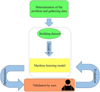
Fig. 2 illustrates the four stages essential for developing a reliable machine learning model for engineering problem-solving. Initially, identification of input features and the target value is crucial, which can be achieved by carefully assessing the base and target spaces. In this study, the base space is for a combination of materials-based and process-based parameters, while the target space is for physical properties, as indicated in Table 1. Note that the effect of tabulated processing parameters at each row in Table 1 has been experimentally estimated by ignoring the effect of other variables. Secondly, compiling a dataset containing information pertinent to the base and target spaces is imperative. It's essential to eliminate any uncorrelated data, especially noise and outlier data, to ensure accurate interpretation of the model.⁴⁵ Thirdly, the appropriate machine learning model to learn from the built dataset should be selected.⁴⁶ Before fitting the learning model, the type and complexity of the model must be considered. Identifying the optimal model before fitting it to the data is challenging. Accordingly, different models were chosen and fitted to the data, and ultimately the best model was selected. In the final step, the built model should be optimized and evaluated to provide the highest quality prediction of the unseen data. This procedure is performed with test data unseen by the machine learning model before the prediction.

Fig. 2 Machine learning procedure for engineering problem-solving.

Table 1 Inputs and target values of the dataset

Variable types	Input features	Effect	Target values
a The variation of the morphology of the fibrous scaffolds with respect to the applied voltage highly depends on the type of materials used. Only the most common effects of voltage have been summarized in Table 1.
Material-based influential parameters	Matrix polymer type, matrix polymer concentration, matrix polymer solvent	High polymer concentration leads to molecular chain entanglements, which overcomes surface tension without fragmenting the jet, resulting in uniform continuous fibers. Higher molecular chain entanglement increases viscosity, which reduces electrospinnability and increases fiber thickness^47,48	Fibers diameter, electrical conductivity
	Conductive polymer type, conductive polymer medium, conductive polymer dopant	Adequate conductivity facilitates charge accumulation, reducing jet eruption voltage. High conductivity may cause unstable multi-jetting from electrical discharge into the ambient atmosphere^49–51
Process-based influential parameters	Voltage^a (kV)	The voltage should be higher than a critical voltage (VC) to overcome the surface tension and to sustain a jet. There is an inverse relationship between voltage and flight duration; increasing voltage shortens flight time, and alter fibers diameter, and, beyond a critical threshold, causes the development of erratic jets and beads^52–54
	Flow rate (ml h^−1)	Above the critical flow rate, an increase in flow rate results in less fiber stretching, a bigger pore size, and a greater fibers diameter^55–57
	Collector rotation speed (rpm)	Thinner fibers are favored by increasing rotation speed of the collector. Decreasing the rotation speed beyond a critical speed promotes the formation of thicker and beaded fibers^58,59
	Distance of the tip (cm)	When the distance is decreased beyond a critical point, it results in thicker fibers and morphological abnormalities. Thinner fibers result from increasing the distance. However, when the distance is raised beyond a critical point, it leads to beaded or fused fiber defects^60–62

---

3. Dataset establishment

3.1. Dataset collection

In the field of tissue engineering, numerous studies have explored 2D conductive scaffolds fabricated using the electrospinning technique.^25,63,64 Polymeric materials are dominant constituents in the fabrication of conductive scaffold materials. Thus, these components have been selected as influential material-based parameters to evaluate relations between constituent materials and the physical properties of the fabricated scaffold. In this regard, 58 samples from the published articles were collected for scaffold conductivity and fibers diameter prediction.^{25,63,65–79} It should be mentioned that numerous experimental datasets could not be utilized due to variations in methodologies employed by researchers. To facilitate comparison of parameters across samples and enable machine learning models to catch their relationships, it is imperative for all parameters within each sample to adhere to a consistent framework. This necessitates gathering data with standardized parameters. As a result, inconsistent data from the dataset was excluded to ensure data integrity.

3.2. Materials and methods

Every material in the collected dataset is assigned to one of the following four categories:

• Matrix polymers.

• Conductive polymers.

• Solvents.

• Conductive polymers' dopants.

The matrix polymers in the dataset include both synthetic polymers, namely polyvinyl alcohol (PVA) and polycaprolactone (PCL), as well as natural polymers such as chitosan and gelatin. The conductive polymers used in this work are polypyrrole (PPy), poly(3,4-ethylene dioxythiophene) (PEDOT), and polyaniline (PANI). Different organic and inorganic solvents, such as distilled water, acetic acid, and chloroform, were used in the reported studies. Different dopants, including sodium para toluene sulfonate (TSNa), camphor sulfonic acid (HCSA), etc., were doped into the conductive polymers to modify their electrical conductivity. The list of materials mentioned and categorized in the collected dataset is represented in Table 2.

Table 2 List of different categories of materials in the collected dataset

Category	Material name
Matrix polymers	Chitosan, PVA, PCL, gelatin etc.
Conductive polymers	PPy, PANI, PEDOT
Solvents	Distilled water, acetic acid, chloroform etc.
Conductive polymers' dopants	TSNa, HCSA, TSA etc.

---

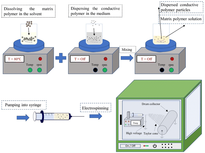
In the fabrication process, the initial step is to dissolve the matrix polymer in its solvent, creating a polymer solution. Next, the conductive polymer is dissolved or dispersed in a suitable liquid medium. Due to the difficulty of dissolving certain conductive polymers, sometimes dispersing them is preferred over dissolution. Subsequently, the conductive solution or suspension is incorporated into the matrix polymer solution.

In addition to material-based parameters, process-based variables also significantly influence the diameter and conductivity of fibers. These encompass applied voltage, flow rate, collector rotation speed, and tip-to-collector distance. The electrospinning process involves preparing a polymer mixture, followed by pumping the polymer solution containing the conductive component through a syringe. Subsequently, nanofibers are produced by ejecting a polymer jet from the tip of a metallic needle. The schematic of the fabrication procedure is represented in Fig. 3.

Fig. 3 A schematic presentation of electrospinning process.

3.3. Base space and target space

The first task before any modeling and optimization is to determine the base and the target spaces of the work. The field of materials science is composed of the following five components:⁸⁰

• Compound.

• Process.

• Structure.

• Properties.

• Performance.

Each of the aforementioned components can be categorized as either a base or target space. In this study, the base space pertains to the compound (materials) and process (electrospinning technique). Conversely, the target space encompasses properties, specifically physical properties such as fiber diameter and electrical conductivity. While other components, such as structure and performance, are relevant, this study will primarily concentrate on the base space of compound and process, and the target space of properties.

3.4. Libraries

In the present study, the whole analysis was carried out using the assistance of Pandas, NumPy, Scikit-learn, TensorFlow, Keras, RDKit, and Seaborn libraries. Pandas and NumPy libraries are often used for the mathematical processing of data. Scikit-learn, TensorFlow, and Keras libraries are used for modeling and tuning. Here, the RDKit package was used to represent polymeric materials as meaningful values to the computer, and finally, the Seaborn library was used to plot figures.

4. Preprocessing

4.1. Imputation

During dataset building, it might happen that some values have not been mentioned or measured in the literature. However, this does not imply that machine learning algorithms cannot be applied to this data.⁸¹ To impute the missing values in a dataset with different strategies, three imputers in the Scikit-learn library can be used: iterative imputer, simple imputer, and KNN imputer.^82,83 All three of these imputers were used to infer the missing values and were subsequently evaluated using some of the data presented. Finally, the best imputer was selected to complete the dataset. The simple imputer is the simplest imputer that uses straightforward strategies to impute the data. These strategies include median, mean, or most frequented. The KNN imputer is derived from the KNN estimator, which considers the ‘k’ number of the closest neighbors to the missing point and replaces the mean value of the ‘k’ nearest neighbors instead of the missing one value. The iterative imputer is a meta-estimator that works with regression or classification estimators and predicts the missing value as a function of other values. The imputers utilized to impute the missing values of the gathered dataset for this work are listed in Table 3 with their imputation R² scores (the R² score was measured between the imputed data, which have been eliminated to compare). The iterative imputer with gradient boosting estimator was selected according to the highest R² score value (0.9342). Following this step, the dataset was devoid of any missing values, making it ready for the subsequent step which involved material representation.

Table 3 Different imputers used with their relevant R² scores

Imputer	Imputing R^2 score
Simple imputer (median)	0.6128
KNN imputer (n_neighbors = 1)	0.8733
Iterative imputer (random forest)	0.9334
Iterative imputer (gradient boosting)	0.9342

---

4.2. Material representation

In machine learning approaches, materials need to be input to the model as numeric data. Thus, converting material names and structures into meaningful numerical representations poses a challenge. Two effective approaches may be used to address this problem. The first method involves assigning a numerical value to the materials' names and structures in a series of discrete numbers, i.e., 0, 1, 2. This solution, known as encoding, is carried out using two main encoders in the Scikit-learn library, namely, ordinal encoder and one hot encoder.⁸⁴ The second solution to address this problem is to represent materials using specific descriptors, such as their physical, mechanical, or magnetic properties. The combination of these descriptors provides meaningful information for the machine learning model to identify the materials.^85,86 Some methods can be utilized to solve this problem, such as fingerprint, SMILES code, coulomb matrix, weighted graph, and other similar approaches.^87–90

In this study, the SMILES code was utilized to represent materials as numeric values for input into the machine learning model. SMILES, a linear notation, uniquely represents chemical compounds as strings over a defined alphabet. This notation employs specific grammar and an alphabet to define the atoms and structure of chemical compounds. As an example, the SMILES string for the chemical known as sodium p-toluenesulfonate compound is written as CC1=CC=C(C=C1)S(=O)(=O)[O⁻][Na⁺].⁹¹

In this study, a simple SMILES enumeration strategy has been employed to represent polymeric and organic materials. There are two possible methods by which the SMILES representation is applied to materials:

• Using a simple enumeration strategy to represent materials in a meaningful numerical matrix.

• Converting the SMILES string to a SMILES convolution fingerprint (SCFP) using either a recurrent neural network (RNN) or a convolutional neural network (CNN); in other words, masking the SMILES string.⁸⁷

In order to enumerate the SMILES strings into a numeric matrix, the first method was used. The numerical values related to the atomic substance quantities, such as degree, charge, chirality, etc., were computed using the RDKit (version 2022.03.3).⁹² One Hot encoder was used to compare all SMILES compounds to the base substance to build the matrix of materials represented by numeric 0 and 1. The base substance could be anything since, when the base substance is changed, all the materials experience a shift and once again have a distinct and unique matrix. In this approach, the base substance's numeric 0 and 1 matrix were produced according to the elements, bounds, and other characteristics that RDKit determined. The input for the encoder consists of sequential symbols describing the chemical properties of the target compound. In other materials, just compared to the base matter, the difference between the target and base matter makes zero in the corresponding value of the representation matrix. The differences could be due to the elements, bounds, charge, etc. Finally, the representation matrix, including all the materials, was generated. Fig. 4 shows the process of material representation by the SMILES representation technique.

Fig. 4 Schematic of SMILES representation procedure.

Using SMILES representation requires basic knowledge about the SMILES alphabet. There are 42 symbols in total to represent the atoms, and original SMILES. There are 21 symbols for atoms consisting of the type of atom, its charge, and its chirality.⁹¹ The other 21 symbols were used to represent the SMILES original. All 42 symbols for SMILES representation are listed in Table 4.

Table 4 SMILES representation alphabets

Feature	Description	Total number
Degree	Degree of unsaturation	5
Charge	Formal charge	1
Chirality	R, S, or others	1
Atom	H, C, O, N, or others	1
NumHs	Total number of H atoms attached to it	1
Valence	Total valence	1
Ring	Whether it is included in a ring	1
Aromaticity	Whether it is included in an aromatic structure	3
Hybridization	s, sp, sp^2, sp^3, sp^3d, sp^3d^2, or others	7
(	Branch start	1
)	Branch end	1
[	Atom or atom group start	1
]	Atom or atom group end	1
.	Ionic bond	1
:	Aromatic bond	1
=	Double bond	1
#	Triple bond	1
	Cis	1
/	Trans	1
@	Chirality (above or below)	1
+	Cation (positive ion)	1
−	Anion (negative ion)	1
Ion charge	Numbers show ionic charge (2–7)	6
Start	Numbers show ring start	1
End	Numbers show ring end	1

---

4.3. Dimensionally reduction

Using SMILES representation, a flattened matrix consisting of nearly 21 000 arrays for each material was provided in this investigation. Numerous columns carry different information depending on the material represented. Processing this data at this volume requires a very high-end resource and significant time. Handling data at this volume demands high-end resources and considerable time. Moreover, the high correlation among the arrays means that many contain redundant information for the model. Consequently, the presence of highly correlated features posed a challenge that required a solution. That was also a non-computational problem because all the features, which included materials and methods, were independent. Principal component analysis (PCA) was implemented to minimize the dimensions and correlations in the data.⁹³ Following the application of the PCA, all the features were mapped onto some new components, which explained the determined identified variance as features carry. Following this, the number of features was reduced to seven components with a variance of 0.999999 compared to the raw data. Another benefit of employing PCA is that the newly mapped components frequently exhibit a Gaussian distribution when the dataset dimensions are reduced using this technique.

4.4. Standardization

After using PCA to reduce the dimensions of the data, different features have various means and standard deviations. These two factors determine the value of each feature. The features must be standard before processing to make all the features comparable for learning models. The standard scaler was used to standardize the features to a mean value of 0 and the same standard deviation.

4.5. Discretization

Using the classification strategy to solve this problem could provide some benefits for improving accuracy, since this strategy simplifies and reduces the complexity of the problem. Firstly, the target values should be confined to specific, defined ranges to solve the problem using classification techniques. Table 5 represents the instruction for classifying the target values in a specific numeric range. After discretization, the problem can be solved with two regression and classification algorithms (a regression algorithm for continuous values and a classification algorithm for discrete target values).

Table 5 Instruction of target values discretization

Target 1		Target 2
Values (nm)	Classes	Values (S cm^−1)	Classes
50–100	1	10^1–10^0	1
100–150	2	10^0–10^−1	0
150–200	3	10^−1–10^−2	−1
200–250	4	10^−2–10^−3	−2
250–300	5	10^−3–10^−4	−3
300–350	6	10^−4–10^−5	−4
350–400	7	10^−5–10^−6	−5
400–450	8	10^−6–10^−7	−6
450–500	9	10^−7–10^−8	−7
500–550	10	<10^−8	−8
550–650	11
650–850	12
850–1200	13
More than 1200	14

---

The next step in the classification task is balancing the data for better learning. Unbalanced data will cause the model to miscalculate the weight of the samples.⁸¹ To overcome this problem, all the target value classes should have the same sample number. Hence, all the samples related to a specific target value are copied to the most frequented target value class number. For the first target, which measures fibers diameter, all the classes should have ten samples, and for the second target, which evaluates conductivity, all the samples should have twenty samples.

4.6. Visualization and correlation

The heatmap correlations between the new components and target values (fibers diameter and conductivity) were plotted in Fig. 5a for continuous target values (regression). While Fig. 5b and c provide the information for discrete target values (classification). Some important information included in the values of the correlations determines the proper machine learning model. The correlation in Fig. 5 is measured as the Pearson coefficient correlation, ranging from −1 to 1.⁹⁴ This value could determine the linearity or non-linearity of the relations between components and target values. The correlation value closer to −1 or 1 indicates linear mode, whereas the closest value to 0 indicates non-linear mode. As observed, all components exhibit correlation values close to 0 for the continuous target 1 (fiber diameter). Clearly, a nonlinear machine learning model is necessary for learning the relations between components and the first target value. Various models were employed, and the most complex one (deep neural network) was chosen to build the optimal model.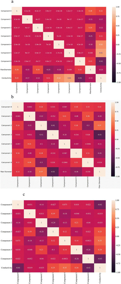

Fig. 5 Heatmap of correlations between new components and target values after dimension reduction (a) continuous targets, (b) discrete target 1, and (c) discrete target 2.

The correlation values indicate the semi-linear relations for the second continuous target (fibers conductivity) (close to |0.5|). As KNN regressor is a non-parametric model, it can be either linear or non-linear based on the fed data and has enough flexibility to find relationships between variables with semi-linear correlation. Consequently, the KNN regressor was selected here as the best machine learning model to learn the relations between data. Further information about this model is provided in Section 5.3.

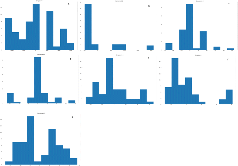
Using PCA, a scatter matrix plot was utilized to inspect the distribution of the new components. Fig. 6 shows that most components have a better distribution than the basic features. It can be related to the PCA application in the dimension reduction step. The distribution of the features plays an essential role in the efficiency of different estimators. For example, the K nearest neighbors' algorithm does not need many preprocessing tasks. On the other hand, the distribution significantly impacts the model performance, particularly in the Gaussian process. Accordingly, the distribution of the features was plotted for visualization and comprehension purposes.

Fig. 6 Histogram of features distribution; (a)–(g): component 0 to 6.

5. Processing

5.1. Machine learning in tissue engineering

In recent decades, modeling and statistical approaches have been employed to model different problems and build predictive models to learn biological, physical, mechanical, and many other properties between variables and predict desired target values.^95–98 Similar to statistical modeling, machine learning techniques also necessitate some understanding of the problem before modeling. However, in contrast to statistical methods, a machine learning model can discern relationships within the provided data without relying on any prior assumptions about the relationships between the variables involved in the problem.⁹⁹

As explained in the previous sections, two tasks were considered to build predictive models to learn the relationship between compounds, processes, and properties. To predict the fibers diameter and conductivity of the fiber in the regression task, an artificial neural network (ANN) and one of the conventional machine learning models named K-nearest neighbors (KNN) regressors have been adopted, respectively. To predict the fibers diameter and conductivity in the classification task, a KNN classifier and a voting classifier were used, respectively. The next section provides some general information about these models.

5.2. Artificial neural network (ANN)

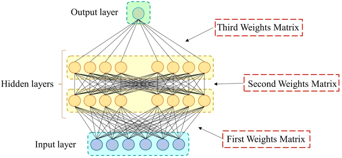
Artificial neural networks have a successful track record in different fields, including materials science and tissue engineering.^39,100–102 ANN was introduced in 1943, inspired by the network of biological neurons in the human brain.¹⁰³ This network comprises artificial neurons interconnected by artificial synapses. Input data is fed into neurons and experiences various mathematical functions. The outputs of neuron can serve as either the final network value (target value) or as input for subsequent layer neurons. The architecture of neural networks is determined by factors such as input, hidden, and output layers; the quantity of neurons; their activation functions; and their solvers. Fig. 7 represents the schematic of a neural network with the input layer, two hidden layers, and the output layer. The corresponding synapse weights each input value to neurons. This makes the model more accurate for target prediction.

Fig. 7 Architecture of artificial neural network with input, output, and hidden layers.

In this context, there are various activation functions named identity, logistic, hyperbolic tangent, relu, etc. The activation function determines the topology of the connection between neurons, scales, and then produces each neuron's output. Table 6 represents the formula for the four mentioned activation functions.¹⁰⁴

Table 6 Different activation functions with their formula.¹⁰⁴

Activation function	Formula
Hyperbolic tangent	f(x) = (exp^x − exp^−x)/(exp^x + exp^−x)
Logistic	f(x) = 1/(1 + exp^−x)
Identity	f(x) = x
Relu	f(x) = max (0, x)

---

Avoiding overfitting is one major challenge in building neural networks. There are two effective methods to solve that:¹⁰⁵

• Using dropout for hidden layers' neurons. In this method, during the learning process (each epoch), each neuron has a determined chance (dropout value) to be inactivated or dropped. It means that inactivated neurons will not be updated during the learning process. This method is conducted to reduce the overfitting of the model.

• Using an early-stop routine. In other words, setting the number of epochs determines the number of iterations during the neural network learning process. However, this method is used to improve the model's performance and avoid underfitting.

Another challenge in neural networks is finding the optimal combination of hyperparameters to build an effective predictive model. Factors such as the number of neurons, hidden layers, activation functions, and dropout percentages can each present individual challenges.¹⁰⁶ In the present study, different combinations of hyperparameters were hired to find the best setting. Table 7 represents the search space for hyperparameter tuning. The search space for these parameters is extensive, making grid searching impractical. Therefore, these parameters were evaluated manually to minimize the mean validation loss. The optimized hyperparameters selected are outlined in Table 7.

Table 7 Hyperparameters' search space and the best setting

Activation function	Upper search space limit	Lower search space limit	Best setting
Number of hidden layers	5	1	2
Number of neurons	10	500	(100, 100)
Activation functions	ReLu	Adam	ReLu
Number of epochs	500	10 000	4200
Dropout percentage	0	20	0

---

Here, a neural network with optimized hyperparameters was fitted to training data to build a predictive model for target 1, which represents the fibers diameter. The model's results will be discussed in the Results and discussion section.

5.3. K-nearest neighbors (KNN)

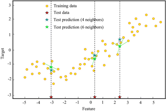
K-nearest neighbors (KNN) stands out as one of the oldest and simplest models in machine learning algorithms. Utilizing distance measurement between all other points and the target, KNN identifies both the nearest and farthest data points. When predicting a new datapoint, it typically assesses the predetermined number of closest neighbors surrounding the target point and calculates the mean of these values for the prediction.¹⁰⁷ The model's approach to learning relations and predicting new data points is illustrated in Fig. 8. Here, neighbor numbers 4 and 6 were randomly selected to enhance comprehension of how the KNN model works and how new data points are predicted. The selection of these numbers is arbitrary, and users can define them by regularizing the ‘n_neighbor’ hyperparameter during model fitting. In a classification task, the model's approach is the same, but when predicting a new datapoint, it considers the most frequented class as the predicted value.

Fig. 8 The KNN model approach to predict a new datapoint.

KNN has a significant advantage over other machine learning models due to its simplicity, making it accessible even to non-experts. There are two principal hyperparameters for this model: the number of neighbors, which controls the complexity of the model; and the way of measuring the distance between data points.¹⁰⁸ By increasing the number of neighbors, the non-linearity of the model decreases. On the other hand, the minimum value for the number of neighbors (n = 1) led to the highest non-linearity of the model. Plotting the validation curve allows for the evaluation of the neighbors' number hyperparameter effect. Furthermore, distance-measuring metrics, such as Manhattan, Euclidean, and Minkowski, are often adopted to measure the distance between data points. This study defaults to using the Minkowski metric.

This model was trained using the training data to capture the relations between variables and make a prediction for target 2, which represents fibers conductivity. In the Results and discussion section, the accuracy of the model and its evaluation will be explored.

5.4. Voting classifier

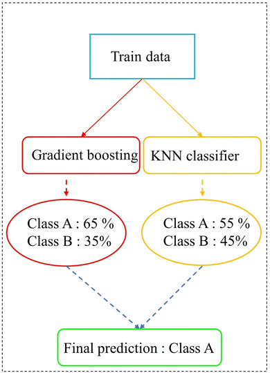
Ensemble methods could combine powerful methods to build predictive models. The voting classifier is the ensemble approach that was employed in this work. Voting ensembles have a simple but powerful strategy to predict. In this method, different classifiers are employed and learned individually from the training data. Each classifier has a specific output prediction. The final prediction is determined by considering the majority's answer. This study uses two classifier estimators: the KNN classifier and the gradient boosting classifier (GB). GB is an ensemble method based on a decision tree estimator. This estimator operates by generating a series of decision trees, and each tree attempts to modify the previous one.¹⁰⁹ Fig. 9 illustrates the schematic of the voting classifier in this study. It was built using the KNN classifier with n_neighbors = 1 and a gradient-boosting classifier with 1000 decision trees.

Fig. 9 Voting regressor instruction to learn.

6. Experimental section

In addition to the data preprocessing, model training and testing, and optimization outlined in the previous section, an experiment was conducted. This experiment involved fabricating PVA and PVA/PPy scaffolds via electrospinning technique to experimentally validate the model predictions. Below, the experimental procedure will be described in detail.

6.1. Materials

Polyvinyl alcohol (PVA) (M_w 70 000, 99% hydrolyzed), pyrrole monomer (reagent grade 98%), anhydrous iron(III) chloride (FeCl₃), and sodium dodecyl sulfate (C₁₂H₂₅NaO₄S) anionic surfactant were purchased from Sigma-Aldrich.

6.2. Polypyrrole synthesis

According to Yussuf et al.,¹¹⁰ polypyrrole (PPy) was polymerized by chemical oxidative polymerization. PPy synthesis was carried out in a 600 ml beaker of oxidant, surfactant, and pyrrole monomer solutions in deionized water (DI water) in a water-ice bath. Table 8 shows the concentration of oxidant, surfactant, and pyrrole monomer in distilled water. Firstly, aqueous solutions of iron chloride (III) and sodium dodecyl sulfate were mixed for 20 min. Then, the pyrrole monomer-solution in DI water was added. Fine black particles of the PPy were formed immediately. The PPy polymerization process was carried out for 4 hours in the ice-water bath. During polymerization, vigorous magnetic stirring was maintained to facilitate the formation of the PPy. Finally, PPy precipitates were filtered using filter paper, washed several times with DI water and ethanol, and dried in an oven at about 40 °C overnight.

Table 8 Materials concentration in the PPy polymerization

Material name	Designated	Concentration (M)
Pyrrole monomer	mPPy	0.05
Ferric chloride	FeCl3	0.1
Sodium dodecyl sulfate	C12H25NaO4S	0.025

---

6.3. Electrospun scaffold fabrication

Initially, a homogenous PVA aqueous solution (10% wt/v) was prepared by magnetically stirring PVA powder in DI water at 80 °C for 4 h. In the next step, to prepare the PVA/5%wt. PPy electrospinning solution, 0.023 g of PPy was added to the PVA solution and magnetically stirred for 2 h. The 2D electrospun scaffold was fabricated using a single nozzle electrospinning apparatus. The solution was pumped at a constant feeding rate of 0.6 ml h⁻¹ from a 5 ml syringe (0.8 mm OD needle) with an applied high voltage of 9.3 kV. The fibers were collected on an aluminium-covered rotating drum placed at 14 cm distance from the needle. The entire electrospinning procedure was carried out at ambient temperature and humidity. To enhance the mechanochemical properties of the fabricated scaffolds, electrospun nanofibers underwent crosslinking using glutaraldehyde in a sealed desiccator saturated with glutaraldehyde vapor. This process involved placing a Petri dish containing 2 ml of aqueous glutaraldehyde solution (25 percent v/v) at the bottom of the desiccator. The nanofiber scaffolds were then positioned on a mesh plate on the upper layer and left for 24 hours at 45 °C.

6.4. Electrospun scaffold characterization

Field-emission scanning electron microscopy (FE-SEM) was used to study the structural morphology of electrospun fibrous scaffolds (FEI NOVA NanoSEM450) at an accelerating voltage of 10 kV. To avoid electron charging, a platinum sputtered layer was applied to samples prior to imaging. The diameters of at least 60 fibers were randomly measured from each picture using ImageJ software, and the results were presented as the average ± standard deviation (D_ave ± SD).

7. Results and discussion

The results of machine learning models were first divided into two evaluation tasks: classification and regression. Initially, the classification models underwent evaluation, followed by the regression models. Subsequently, the experimental results were presented, and the machine learning models were assessed by comparing the predicted diameter with the actual fiber diameters of PVA and PVA/PPy electrospun scaffolds.

7.1. Classification models

Two classification models were used to build predictive models to learn the dataset's relationships. Learning the relations between the features and the first target (fibers diameter) was performed using an ensemble voting classifier with the hyperparameters previously mentioned. The result of the built model on the data is represented in Table 9.

Table 9 Voting classifier model scores for fibers diameter prediction

Metrics	Score
Mean cross validation	0.9841
Cross validation STD	0.0224
Test score	0.9143
Balanced accuracy	0.9478

---

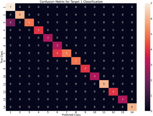
The results presented in Table 9 demonstrate the efficacy of the voting classifier, suggesting that the model was constructed with optimal complexity for the problem. Analysis of Fig. 5 reveals a Pearson correlation between components and the target value, indicating a semi-linear model. Moreover, the built model closely aligns with the actual function of the problem under study. Fig. 10 illustrates the confusion matrix for the fibers diameter classifier for further assessment.

Fig. 10 Confusion matrix for target 1 classifier.

As stated above, there are 14 different classes (classifying the target values by discretization). Upon inspecting the confusion matrix for the voting classifier, it becomes evident that prediction errors were limited to only two out of the 14 classes. A key finding is that these two errors belong to two classes in a row (mostly classes 6 and 7), not in classes with further distance, indicating there are no significant errors of concern; however, there is undoubtedly room for improving the model's performance. It was expected that most of the predicted classes would match the actual classes because of the good scores in Table 9.

A KNN classifier with n_neighbor = 1 was developed to learn the latent relationships between the parameters and the fibers conductivity. The model evaluation was performed, and all the required scores were measured and tabulated in Table 10.

Table 10 KNN classifier model scores for fibers conductivity prediction

Metrics	Score
Mean cross validation	1.0
Cross validation STD	0.0
Test score	1.0
Balanced accuracy	1.0

---

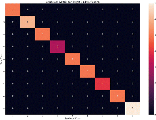
There are excellent scores for the predictive model KNN with the highest complexity (n_neighbors = 1). These results showcase optimal data learning, identifying nearly all latent relations. The result indicates that the KNN classifier is the best possible solution for this problem. Moreover, the confusion matrix shown in Fig. 11 is an essential additional element that needs to be evaluated.

Fig. 11 Confusion matrix for target 2 classifier.

There are no errors in the confusion matrix for the predictive model for target 2. As expected, all the predicted values match true values due to the excellent scores measured and represented in Table 10. It can be considered that this model works perfectly, and there is no room for any improvement. Given the complexity of the problem at hand, the model's performance is outstanding. Despite being trained on only about 45 samples; it functions as a general model with remarkable potential for generalization.

As previously mentioned, categorizing target values into discrete ones provides certain advantages, such as simplifying the complexity of the problem. However, it became apparent that regression tasks could predict the exact target value more accurately, albeit with some uncertainty. Classification facilitated the building of a predictive model capable of learning the relationship between compound, process, and properties across a mere 45 samples. Nonetheless, regression models were utilized, and their outcomes are elaborated upon in the subsequent section.

7.2. Regression models

A neural network regressor was employed to provide a predictive model to learn the relation for capturing the parameters influencing the fibers diameter. The neural network architecture was finally found to optimize the model's performance through several tries and errors. Table 11 represents the results of neural network regressor learning.

Table 11 Neural network's results for target one prediction

Metrics	Value
Mean cross validation absolute percentage error	13.91
Mean cross validation absolute percentage error STD	7.34
Mean absolute error	46.96
Explained variance score	0.56
Max error	412.92

---

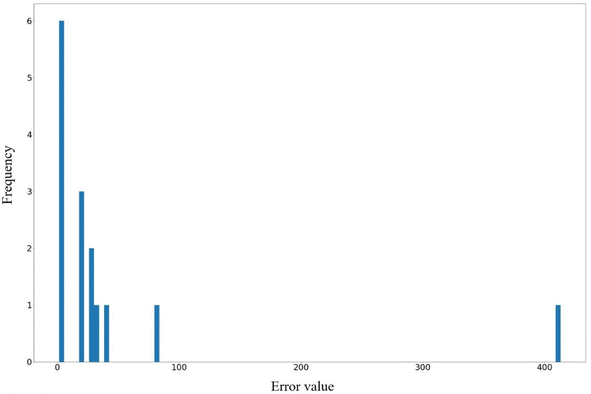
The results demonstrate that the designed neural network works effectively on the data. The volume of samples should first be considered to solve this regression problem. Managing this problem with a machine learning approach was challenged by the scarcity of available data. The limitation in samples stemmed from the varied methodologies employed by researchers, necessitating data collection under uniform procedures and parameters. Consequently, only a limited number of samples were obtained through consistent procedures. Subsequently, the model utilized this data as input to discern the latent relationships between compounds, processes, and properties. Therefore, the performance of the model to capture these relations proves excellent. The histogram of the prediction error shown in Fig. 12 has been plotted to evaluate the maximum error of the prediction. It shows that the maximum error, which is represented as a model's result, just occurred for one sample, and all the other errors are less than 100 nm. The value of the maximum error could be related to an outlier data point, which has led to an increase in the mean absolute error. If this maximum error is not considered, the mean absolute error is less than 46.96 nm. Consequently, the built neural network model works well even with a very small dataset.

Fig. 12 Histogram of prediction error frequency for neural network in target one prediction.

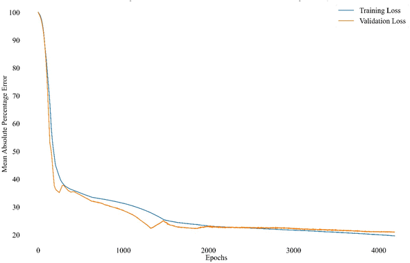
During the neural network's learning process, the training and validation losses were captured. Fig. 13 displays the changes in the values of these two parameters. As illustrated, the model's learning and validation loss, measured by the mean absolute percentage error, reach a plateau approximately after 4200 epochs, indicating that the model could attain stability and operate effectively with the specified scores. The steeper decrease in slopes during the initial epochs suggests that the model begins learning the relationships with a robust approach, ultimately yielding favorable results over the four thousand epochs. Note that the validation loss is lower than the training loss, which is unacceptable. The proportion of the two mentioned loss factors renders the model reliable after about 2000 epochs.

Fig. 13 Training and validation loss for neural network.

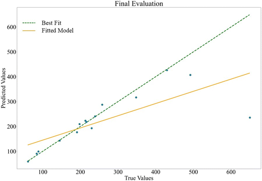
Fig. 14 illustrates the prediction error graph that was used to evaluate the distribution of predicted and true target values. The higher related predicted and true values indicate that the model works correctly. Consequently, the 45° line was plotted, and the fitted line on the distribution of predicted and true values has been hypothesized. The closeness of these two lines indicates a criterion of the model's accuracy, which is usually measured as R² in regression tasks. The measured R² score for the neural network is shown in Fig. 12. It should be noted that the test size of the data was 0.2, which means the model could self-evaluate on just about ten samples. Although the R² value close to 0.723 is relatively low, it is suitable for such a low number of test samples. Note that the model works on this very small dataset by considering the cross-validation and R² score as two factors of the neural network score. The error histogram plot reveals an outlier with a significant mismatching error, consistent with the prediction error plot where one predicted value deviates considerably from the 45° line. Eliminating this outlier leads to a dramatic improvement in model scores, potentially resulting in an R² score exceeding 0.8. Therefore, the model displays promising capability and accuracy.

Fig. 14 Prediction error plot for neural network model in fibers diameter prediction.

Fibers' conductivity prediction was performed using a KNN regressor. Some regression algorithms were used to capture the relationships between features and fibers conductivity. In all cases, the models were unstable, and the scores varied widely. These changes occurred because of the inadequate sample size for the regression task for fibers conductivity prediction. It indicates that the collected dataset cannot cover all the system information that was tried to be found. To solve this problem, a larger sample for the dataset should be collected.

However, the information in the dataset could not provide enough knowledge for the machine learning models. The KNN regressor with ‘neighbors’ number’ = 2 was fitted to learn from the training data. The cross-validation score and standard deviation, plus the train and test scores of the model, are represented in Table 12.

Table 12 KNN regressor scores for fibers conductivity prediction

Metrics	Value
Train score	0.998
Test score (R^2 score)	0.965
Mean cross validation score	0.972
Mean cross validation STD	0.019

---

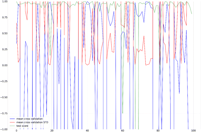
According to the presented analysis, the scores seem to be excellent, but that is only one of the 20 different states determined by random state parameters. By changing the random state in the range of 1 to 20, the scores mentioned in Table 12 vary drastically. Different scores with different random states indicate that the sampling is very decisive in the final scores, which means different training samples provide independent knowledge for the model and some space of problems remains uncovered. The effect of different random states (sampling) on the model learning could be seen by plotting the changes in the mentioned scores for the different random states. Fig. 15 shows the scores in Table 12, except for the training score, to figure out the effect of sampling in this dataset.

Fig. 15 Different model's score with different random states for KNN regressor.

The scores in Table 12 could change drastically due to incomplete data in the dataset for the regressor model to predict fibers conductivity. It indicates that the model has no generalized performance. The model's inability indicates the imperfect capture of the relations corresponding to the conductivity of fibers. Although the model fits the data, it will work more efficiently on data from a larger sample size with additional information.

7.3. Predicted vs. experimented values

FE-SEM micrographs are displayed in Fig. 16. It is evident that the addition of PPy has led to an increase in the mean diameter of PVA fibers from 513 nm to 547 nm. An increase in the electrical conductivity of the solution and, hence, a reduction in the electrospun fibers diameter is expected by the addition of PPy. On the other hand, during experimentation, it was observed that the presence of PPy increased the solution viscosity, which results in an increase in fiber diameter during electrospinning.^13,111 Hence, the addition of PPy has a two-fold effect. As the mean fiber diameter increased in the presence of PPy, it can be concluded that the increase in viscosity predominates over the increase in electrical conductivity. The developed model accurately estimated this trend in fiber diameter change. Moreover, the model predicted the PVA and PVA/PPy scaffolds fiber diameters to be 551 nm and 577 nm, respectively, exhibiting the model's high potential for accuracy.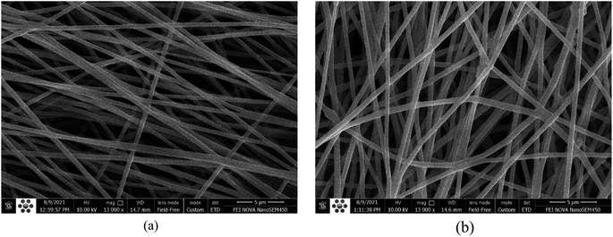

Fig. 16 SEM images of (a) PVA and (b) PVA/5%wt. PPy electrospun scaffolds with a fibrillar structure.

8. Conclusions

The tuning of physical properties in electrospun scaffolds is essential for their application in the tissue engineering field. In this study, a machine learning approach was used to predict the fibers diameter and conductivity of 2D scaffolds based on their material and process parameters. Two different tasks were used: classification and regression. In the classification task, for the prediction of fibers diameter and conductivity, the voting classifier and K-neighbors classifier were used, respectively. In the regression task, the artificial neural network and K neighbors regressor were used to predict the fibers diameter and conductivity. The key aspects and main results of our studied models are summarized here:

• Two classification models have balanced accuracy values of 0.9478 and 1.0 for predicting fibers diameter and conductivity class, respectively. The cross-validation scores of the two classification models were 0.9841 and 1.0, respectively. The confusion matrix was plotted to assess the errors in predicting classes for two targets. In the prediction of fibers' diameter, two errors were observed across two consecutive classes. Conversely, in the prediction of fibers' conductivity, no errors were evident in the confusion matrix, indicating the accurate functioning of the classification models.

• In the regression task, the R² scores were 0.723 and 0.965 for fibers diameter and conductivity prediction, respectively. The effect of the outlier datapoint on the reduction of the R² score of the neural network was discussed. An absolute error histogram was plotted to assess model errors, and the influence of the outlier datapoint was highlighted, resulting in an elevation of the mean absolute error of the constructed neural network. Generally, the neural network performed properly on the very small collected dataset (without considering the outlier datapoint). The K neighbors regressor was trained on training data, but the model has fluctuating performance with different samples because of inadequate data information for capturing the relations between parameters.

• The experimental parameters of electrospinning polymeric scaffolds of PVA and PVA/5%wt. PPy were compared with the developed machine learning model, and it was proved that the model could predict the actual values of fibers diameter with high accuracy.

• Once proper microstructural features are identified for a given 2D polymeric scaffold, the machine learning approach presented in this study can be employed to predict and tune the physical properties of the sample before the scoping exercise, without the need for costly and detailed characterizations.

• The machine learning approach proposed in this study could play a crucial role in establishing a robust foundation for the design of 2D polymeric scaffolds. This could result in faster elucidation of process–structure–property relationships and expedite the discovery of high-performance biomaterials.

• Our finding highlights the tremendous potential of machine learning algorithms for the automated prediction of the fiber diameter and conductivity of 2D scaffolds based on their material-based and process-based parameters. Such great potential holds the promise of spreading the capabilities of the studied prediction model across both academia and industry.

• Even though environmental factors such as temperature and humidity can affect the procedure, they have been largely disregarded in the majority of previous research studies and cannot be studied due to their unavailability.

Data availability

The research data will be available from the corresponding authors upon request.

Author contributions

Conceptualization: M. H. G.; methodology: M. H. G. and M. S. V.; software: M. H. G. and M. S. V.; validation: M. H. G. and M. S. V.; investigation: M. H. G. and F. H.; resources: F. P. and S. A. S. E.; data curation: M. H. G. and M. S. V.; writing – original draft: M. H. G., M. R. B, and F. H.; writing – review & editing: M. H. G., M. R. B. and F. P.; Supervision: F. P. and S. A. S. E.

Conflicts of interest

The authors declare no potential conflicts of interest with respect to the research, authorship, and/or publication of this article.

Acknowledgements

This research did not receive any specific grants from funding agencies in the public, commercial, or not-for-profit sectors. The authors would like to thank Professor Aldo R. Boccaccini (FAU, Erlangen-Nuremberg, Germany) for his valuable input and helpful discussions.

References

1. A. Khademhosseini and R. Langer, A decade of progress in tissue engineering, Nat. Protoc., 2016, 11, 1775–1781,  DOI:10.1038/nprot.2016.123.
2. R. D. Rusk, Science, Educ. Forum., 1950, 15, 119–120,  DOI:10.1080/00131725009342110.
3. S. Caddeo, M. Boffito and S. Sartori, Tissue engineering approaches in the design of healthy and pathological in vitro tissue models, Front. Bioeng. Biotechnol., 2017, 5, 1–22,  DOI:10.3389/fbioe.2017.00040.
4. F. J. O'Brien, Biomaterials & scaffolds for tissue engineering, Mater. Today, 2011, 14, 88–95,  DOI:10.1016/S1369-7021(11)70058-X.
5. M. Okamoto, The Role of Scaffolds in Tissue Engineering, Elsevier Ltd, 2019,  DOI:10.1016/B978-0-08-102563-5.00002-2.
6. M. Rahmati, D. K. Mills, A. M. Urbanska, M. R. Saeb, J. R. Venugopal, S. Ramakrishna and M. Mozafari, Electrospinning for tissue engineering applications, Prog. Mater. Sci., 2021, 117, 100721,  DOI:10.1016/j.pmatsci.2020.100721.
7. R. Chaudhari, P. K. Loharkar and A. Ingle, Medical Applications of Rapid Prototyping Technology, in Recent Advances in Industrial Production, Springer, 2022, pp. 241–250.
8. Z. Shahbazarab, A. Teimouri, A. N. Chermahini and M. Azadi, Fabrication and characterization of nanobiocomposite scaffold of zein/chitosan/nanohydroxyapatite prepared by freeze-drying method for bone tissue engineering, Int. J. Biol. Macromol., 2018, 108, 1017–1027.
9. C. A. Martínez-Pérez, I. Olivas-Armendariz, J. S. Castro-Carmona and P. E. García-Casillas, Scaffolds for tissue engineering via thermally induced phase separation, Adv. Regen. Med., 2011, 35, 275–294.
10. A. Prasad, M. R. Sankar and V. Katiyar, State of art on solvent casting particulate leaching method for orthopedic scaffoldsfabrication, Mater. Today: Proc., 2017, 4, 898–907.
11. M. Costantini and A. Barbetta, Gas foaming technologies for 3D scaffold engineering, in Functional 3D Tissue Engineering Scaffolds, Elsevier, 2018, pp. 127–149.
12. T. R. Ger, H. T. Huang, C. Y. Huang, K. S. Hu, J. Y. Lai, J. Y. Chen and M. F. Lai, Study of polyvinyl alcohol nanofibrous membrane by electrospinning as a magnetic nanoparticle delivery approach, J. Appl. Phys., 2014, 115, 2012–2015,  DOI:10.1063/1.4867600.
13. I. S. Chronakis, S. Grapenson and A. Jakob, Conductive polypyrrole nanofibers via electrospinning: Electrical and morphological properties, Polymer, 2006, 47, 1597–1603,  DOI:10.1016/j.polymer.2006.01.032.
14. N. Bhardwaj and S. C. Kundu, Electrospinning: A fascinating fiber fabrication technique, Biotechnol. Adv., 2010, 28, 325–347,  DOI:10.1016/j.biotechadv.2010.01.004.
15. J. Wu, L. Xie, W. Z. Y. Lin and Q. Chen, Biomimetic nanofibrous scaffolds for neural tissue engineering and drug development, Drug Discovery Today, 2017, 22, 1375–1384,  DOI:10.1016/j.drudis.2017.03.007.
16. M. Solazzo, F. J. O’Brien, V. Nicolosi and M. G. Monaghan, The rationale and emergence of electroconductive biomaterial scaffolds in cardiac tissue engineering, APL Bioeng., 2019, 3, 041501,  DOI:10.1063/1.5116579.
17. P. Sikorski, Electroconductive scaffolds for tissue engineering applications, Biomater. Sci., 2020, 8, 5583–5588,  10.1039/d0bm01176b.
18. H. Nekounam, S. Gholizadeh, Z. Allahyari, H. Samadian, N. Nazeri, M. A. Shokrgozar and R. Faridi-Majidi, Electroconductive scaffolds for tissue regeneration: Current opportunities, pitfalls, and potential solutions, Mater. Res. Bull., 2021, 134, 111083,  DOI:10.1016/j.materresbull.2020.111083.
19. M. Hatamzadeh, R. Sarvari, B. Massoumi, S. Agbolaghi and F. Samadian, Liver tissue engineering via hyperbranched polypyrrole scaffolds, Int. J. Polym. Mater. Polym. Biomater., 2020, 69, 1112–1122,  DOI:10.1080/00914037.2019.1667800.
20. G. Massaglia, A. Chiodoni, S. L. Marasso, C. F. Pirri and M. Quaglio, Electrical conductivity modulation of crosslinked composite nanofibers based on PEO and PEDOT:PSS, J. Nanomater., 2018, 2018, 3286901,  DOI:10.1155/2018/3286901.
21. S. Varnaite-Žuravliova, N. Savest, A. Abraitiene, J. Baltušnikaite-Guzaitiene and A. Krumme, Investigation of influence of conductivity on the polyaniline fiber mats, produced via electrospinning, Mater. Res. Express, 2018, 5, 055308,  DOI:10.1088/2053-1591/aac4ea.
22. S. E. Noriega, G. I. Hasanova, M. J. Schneider, G. F. Larsen and A. Subramanian, Effect of fiber diameter on the spreading, proliferation and differentiation of chondrocytes on electrospun chitosan matrices, Cells Tissues Organs, 2012, 195, 207–221,  DOI:10.1159/000325144.
23. M. Chen, P. K. Patra, S. B. Warner and S. Bhowmick, Role of fiber diameter in adhesion and proliferation of NIH 3T3 fibroblast on electrospun polycaprolactone scaffolds, Tissue Eng., 2007, 13, 579–587,  DOI:10.1089/ten.2006.0205.
24. T. Hodgkinson, X. F. Yuan and A. Bayat, Electrospun silk fibroin fiber diameter influences in vitro dermal fibroblast behavior and promotes healing of ex vivo wound models, J. Tissue Eng., 2014, 5, 1–13,  DOI:10.1177/2041731414551661.
25. A. Babaie, B. Bakhshandeh, A. Abedi, J. Mohammadnejad, I. Shabani, A. Ardeshirylajimi, S. Reza Moosavi, J. Amini and L. Tayebi, Synergistic effects of conductive PVA/PEDOT electrospun scaffolds and electrical stimulation for more effective neural tissue engineering, Eur. Polym. J., 2020, 140, 110051,  DOI:10.1016/j.eurpolymj.2020.110051.
26. K. Li, S. Zhang, S. Wang, F. Zhu, M. Liu, X. Gu, P. Li and Y. Fan, Positive Effect of Magnetic-Conductive Bifunctional Fibrous Scaffolds on Guiding Double Electrical and Magnetic Stimulations to Pre-Osteoblasts, J. Biomed. Nanotechnol., 2019, 15, 477–486,  DOI:10.1166/jbn.2019.2708.
27. M. N. Pervez, W. S. Yeo, M. Mishu, M. Rahman, M. E. Talukder, H. Roy, M. S. Islam, Y. Zhao, Y. Cai and G. K. Stylios, Electrospun nanofiber membrane diameter prediction using a combined response surface methodology and machine learning approach, Sci. Rep., 2023, 13, 1–14.
28. M. N. Pervez, W. S. Yeo, M. R. Mishu, A. Buonerba, Y. Zhao, Y. Cai, L. Lin, G. K. Stylios and V. Naddeo, Prediction of the diameter of biodegradable electrospun nanofiber membranes: An integrated framework of taguchi design and machine learning, J. Polym. Environ., 2023, 1–17.
29. S. Sarma, A. K. Verma, S. S. Phadkule and M. Saharia, Towards an interpretable machine learning model for electrospun polyvinylidene fluoride (PVDF) fiber properties, Comput. Mater. Sci., 2022, 213, 111661.
30. M. H. Golbabaei, M. S. Varnoosfaderani, A. Zare and H. Salari, Performance Analysis of Anode-Supported Solid Oxide Fuel Cells : A Machine Learning Approach, Materials, 2022, 15, 1–26.
31. J. Wei, X. Chu, X. Y. Sun, K. Xu, H. X. Deng, J. Chen, Z. Wei and M. Lei, Machine learning in materials science, InfoMat, 2019, 1, 338–358,  DOI:10.1002/inf2.12028.
32. Y. Xu, Y. Zhou, P. Sekula and L. Ding, Machine learning in construction: From shallow to deep learning, Dev. Built Environ., 2021, 6, 100045,  DOI:10.1016/j.dibe.2021.100045.
33. M. Mowbray, T. Savage, C. Wu, Z. Song, B. A. Cho, E. A. Del Rio-Chanona and D. Zhang, Machine learning for biochemical engineering: A review, Biochem. Eng. J., 2021, 172, 108054,  DOI:10.1016/j.bej.2021.108054.
34. G. D. Goh, S. L. Sing and W. Y. Yeong, A Review on Machine Learning in 3D Printing: Applications, Potential, and Challenges, Springer Netherlands, 2021,  DOI:10.1007/s10462-020-09876-9.
35. D. Solyali, A comparative analysis of machine learning approaches for short-/long-term electricity load forecasting in Cyprus, Sustain, 2020, 12, 3612,  DOI:10.3390/SU12093612.
36. M. Masud, N. Sikder, A. Al Nahid, A. K. Bairagi and M. A. Alzain, A machine learning approach to diagnosing lung and colon cancer using a deep learning-based classification framework, Sensors, 2021, 21, 1–21,  DOI:10.3390/s21030748.
37. G. Wang, P. Pu and T. Shen, An efficient gene bigdata analysis using machine learning algorithms, Multimed. Tools Appl., 2020, 79, 9847–9870,  DOI:10.1007/s11042-019-08358-7.
38. L. Y. Sujeeun, N. Goonoo, H. Ramphul, I. Chummun, F. Gimié, S. Baichoo and A. Bhaw-Luximon, Correlating in vitro performance with physico-chemical characteristics of nanofibrous scaffolds for skin tissue engineering using supervised machine learning algorithms: Scaffolds and machine learning, R. Soc. Open Sci., 2020, 7 DOI:10.1098/rsos.201293rsos201293.
39. E. Entekhabi, M. H. Nazarpak, M. Sedighi and A. Kazemzadeh, Predicting degradation rate of genipin cross-linked gelatin scaffolds with machine learning, Mater. Sci. Eng. C, 2020, 107, 110362.
40. J. Doshi and D. H. Reneker, Electrospinning process and applications of electrospun fibers, J. Electrost., 1995, 35, 151–160.
41. M. Ziabari, V. Mottaghitalab and A. K. Haghi, Application of direct tracking method for measuring electrospun nanofiber diameter, Braz. J. Chem. Eng., 2009, 26, 53–62.
42. S.-C. Wong, A. Baji and S. Leng, Effect of fiber diameter on tensile properties of electrospun poly (ε-caprolactone), Polymer, 2008, 49, 4713–4722.
43. Y. J. Ryu, H. Y. Kim, K. H. Lee, H. C. Park and D. R. Lee, Transport properties of electrospun nylon 6 nonwoven mats, Eur. Polym. J., 2003, 39, 1883–1889.
44. M. Alloghani, D. Al-Jumeily, J. Mustafina, A. Hussain and A. J. Aljaaf, A Systematic Review on Supervised and Unsupervised Machine Learning Algorithms for Data, Science, 2020, 3–21,  DOI:10.1007/978-3-030-22475-2_1.
45. V. Hodge and J. Austin, A Survey of Outlier Detection Methodologies, Artif. Intell. Rev., 2004, 22, 85–126,  DOI:10.1023/B:AIRE.0000045502.10941.a9.
46. V. Tshitoyan, J. Dagdelen, L. Weston, A. Dunn, Z. Rong, O. Kononova, K. A. Persson, G. Ceder and A. Jain, Unsupervised word embeddings capture latent knowledge from materials science literature, Nature, 2019, 571, 95–98.
47. J. Lannutti, D. Reneker, T. Ma, D. Tomasko and D. Farson, Electrospinning for tissue engineering scaffolds, Mater. Sci. Eng. C, 2007, 27, 504–509.
48. S. Haider, Y. Al-Zeghayer, F. A. Ahmed Ali, A. Haider, A. Mahmood, W. A. Al-Masry, M. Imran and M. O. Aijaz, Highly aligned narrow diameter chitosan electrospun nanofibers, J. Polym. Res., 2013, 20, 1–11.
49. B. Sun, Y. Z. Long, H. D. Zhang, M. M. Li, J. L. Duvail, X. Y. Jiang and H. L. Yin, Advances in three-dimensional nanofibrous macrostructures via electrospinning, Prog. Polym. Sci., 2014, 39, 862–890.
50. C. J. Angammana and S. H. Jayaram, Analysis of the effects of solution conductivity on electrospinning process and fiber morphology, IEEE Trans. Ind. Appl., 2011, 47, 1109–1117.
51. J. S. Choi, S. W. Lee, L. Jeong, S.-H. Bae, B. C. Min, J. H. Youk and W. H. Park, Effect of organosoluble salts on the nanofibrous structure of electrospun poly (3-hydroxybutyrate-co-3-hydroxyvalerate), Int. J. Biol. Macromol., 2004, 34, 249–256.
52. T. J. Sill and H. J. B. Von Recum, Electrospinning for tissue engineering and drug delivery, Biomaterials, 2008, 29, 1989–2006.
53. A. Haider, S. Haider and I.-K. Kang, A comprehensive review summarizing the effect of electrospinning parameters and potential applications of nanofibers in biomedical and biotechnology, Arabian J. Chem., 2018, 11, 1165–1188,  DOI:10.1016/j.arabjc.2015.11.015.
54. J. M. Deitzel, J. Kleinmeyer, D. E. A. Harris and N. C. B. Tan, The effect of processing variables on the morphology of electrospun nanofibers and textiles, Polymer, 2001, 42, 261–272.
55. S. Zargham, S. Bazgir, A. Tavakoli, A. S. Rashidi and R. Damerchely, The effect of flow rate on morphology and deposition area of electrospun nylon 6 nanofiber, J. Eng. Fibers Fabr., 2012, 7, 155892501200700400.
56. S. Megelski, J. S. Stephens, D. B. Chase and J. F. Rabolt, Micro-and nanostructured surface morphology on electrospun polymer fibers, Macromolecules, 2002, 35, 8456–8466.
57. Z. Li and C. Wang, One-dimensional Nanostructures: Electrospinning Technique and Unique Nanofibers, Springer, 2013.
58. Z. A. Alhasssan, Y. S. Burezq, R. Nair and N. Shehata, Polyvinylidene difluoride piezoelectric electrospun nanofibers: Review in synthesis, fabrication, characterizations, and applications, J. Nanomater., 2018, 2018, 1–12,  DOI:10.1155/2018/8164185.
59. J. Xue, J. Xie, W. Liu and Y. Xia, Electrospun nanofibers: new concepts, materials, and applications, Acc. Chem. Res., 2017, 50, 1976–1987.
60. K. P. Matabola and R. M. Moutloali, The influence of electrospinning parameters on the morphology and diameter of poly (vinyledene fluoride) nanofibers-effect of sodium chloride, J. Mater. Sci., 2013, 48, 5475–5482.
61. T. Wang and S. Kumar, Electrospinning of polyacrylonitrile nanofibers, J. Appl. Polym. Sci., 2006, 102, 1023–1029.
62. Y. Zheng, S. Xie and Y. Zeng, Electric field distribution and jet motion in electrospinning process: from needle to hole, J. Mater. Sci., 2013, 48, 6647–6655.
63. Y. Cong, S. Liu and H. Chen, Fabrication of conductive polypyrrole nanofibers by electrospinning, J. Nanomater., 2013, 2013, 1–7,  DOI:10.1155/2013/148347.
64. H. Farkhondehnia, M. Amani Tehran and F. Zamani, Fabrication of Biocompatible PLGA/PCL/PANI Nanofibrous Scaffolds with Electrical Excitability, Fibers Polym., 2018, 19, 1813–1819,  DOI:10.1007/s12221-018-8265-1.
65. M. Li, Y. Guo, Y. Wei, A. G. MacDiarmid and P. I. Lelkes, Electrospinning polyaniline-contained gelatin nanofibers for tissue engineering applications, Biomaterials, 2006, 27, 2705–2715,  DOI:10.1016/j.biomaterials.2005.11.037.
66. E. M. Materón, C. M. Miyazaki, O. Carr, N. Joshi, P. H. S. Picciani, C. J. Dalmaschio, F. Davis and F. M. Shimizu, Magnetic nanoparticles in biomedical applications: A review, Appl. Surf. Sci. Adv., 2021, 6, 100163.
67. Y. Liang and J. C. H. Goh, Polypyrrole-Incorporated Conducting Constructs for Tissue Engineering Applications: A Review, Bioelectricity, 2020, 2, 101–119,  DOI:10.1089/bioe.2020.0010.
68. M. C. Chen, Y. C. Sun and Y. H. Chen, Electrically conductive nanofibers with highly oriented structures and their potential application in skeletal muscle tissue engineering, Acta Biomater., 2013, 9, 5562–5572,  DOI:10.1016/j.actbio.2012.10.024.
69. X. X. Wang, G. F. Yu, J. Zhang, M. Yu, S. Ramakrishna and Y. Z. Long, Conductive polymer ultrafine fibers via electrospinning: Preparation, physical properties and applications, Prog. Mater. Sci., 2021, 115, 100704,  DOI:10.1016/j.pmatsci.2020.100704.
70. T. Blachowicz and A. Ehrmann, Conductive Electrospun Nanofiber Mats Tomasz, 2019.
71. Q. Z. Yu, M. M. Shi, M. Deng, M. Wang and H. Z. Chen, Morphology and conductivity of polyaniline sub-micron fibers prepared by electrospinning, Mater. Sci. Eng. B Solid-State Mater. Adv. Technol., 2008, 150, 70–76,  DOI:10.1016/j.mseb.2008.02.008.
72. A. Abedi, M. Hasanzadeh and L. Tayebi, Conductive nanofibrous Chitosan/PEDOT:PSS tissue engineering scaffolds, Mater. Chem. Phys., 2019, 237, 121882,  DOI:10.1016/j.matchemphys.2019.121882.
73. P. Moutsatsou, K. Coopman and S. Georgiadou, Chitosan & Conductive PANI/Chitosan Composite Nanofibers - Evaluation of Antibacterial Properties, Curr. Nanomater., 2018, 4, 6–20,  DOI:10.2174/1573413714666181114110651.
74. J. C. Bittencourt, B. H. de Santana Gois, V. J. Rodrigues de Oliveira, D. L. da Silva Agostini and C. de Almeida Olivati, Gas sensor for ammonia detection based on poly(vinyl alcohol) and polyaniline electrospun, J. Appl. Polym. Sci., 2019, 136, 26–29,  DOI:10.1002/app.47288.
75. Y. Zhang and G. C. Rutledge, Electrical conductivity of electrospun polyaniline and polyaniline-blend fibers and mats, Fiber Society 2012 Fall Meeting and Technical Conference in Partnership with Polymer Fibers 2012: Rediscovering Fibers in the 21st Century, 2012.
76. C. A. Chapman, P. R. Ho, R. W. Udangawa, J. C. Silva, P. E. Mikael, C. A. V. Rodrigues, J. M. S. Cabral, J. M. F. Morgado, F. C. Ferreira and R. J. Linhardt, Polyaniline-polycaprolactone blended nano fi bers for neural cell culture, Eur. Polym. J., 2019, 117, 28–37.
77. D. Kai, M. P. Prabhakaran, G. Jin and S. Ramakrishna, Polypyrrole-contained electrospun conductive nanofibrous membranes for cardiac tissue engineering, J. Biomed. Mater. Res., Part A, 2011, 99(A), 376–385,  DOI:10.1002/jbm.a.33200.
78. K. Low, C. B. Horner, C. Li, G. Ico, W. Bosze, N. V. Myung and J. Nam, Composition-dependent sensing mechanism of electrospun conductive polymer composite nanofibers, Sens. Actuators, B, 2015, 207, 235–242,  DOI:10.1016/j.snb.2014.09.121.
79. V. J. Babu, D. V. B. Murthy, V. Subramanian, V. R. K. Murthy, T. S. Natarajan and S. Ramakrishna, Microwave Hall mobility and electrical properties of electrospun polymer nanofibers, J. Appl. Phys., 2011, 109, 074306,  DOI:10.1063/1.3556456.
80. W. F. Smith, J. Hashemi and F. Presuel-Moreno, Foundations of Materials Science and Engineering, McGraw-hill, New York, 2006.
81. M. W. Libbrecht and W. S. Noble, Machine learning applications in genetics and genomics, Nat. Rev. Genet., 2015, 16, 321–332.
82. O. Altukhova, Choice of method imputation missing values for obstetrics clinical data, Procedia Comput. Sci., 2020, 176, 976–984.
83. M. S. Santos, P. H. Abreu, S. Wilk and J. Santos, How distance metrics influence missing data imputation with k-nearest neighbours, Pattern Recognit. Lett., 2020, 136, 111–119.
84. A. C. H. Choong and N. K. Lee, Evaluation of convolutionary neural networks modeling of DNA sequences using ordinal versus one-hot encoding method, in 2017 International Conference on Computer and Drone Applications, IEEE, 2017, pp. 60–65.
85. A. Seko, H. Hayashi, K. Nakayama, A. Takahashi and I. Tanaka, Representation of compounds for machine-learning prediction of physical properties, Phys. Rev. B, 2017, 95, 144110.
86. J. E. Herr, K. Koh, K. Yao and J. Parkhill, Compressing physics with an autoencoder: Creating an atomic species representation to improve machine learning models in the chemical sciences, J. Chem. Phys., 2019, 151, 84103.
87. E. Paradis and K. Schliep, ape 5.0: an environment for modern phylogenetics and evolutionary analyses in R, Bioinformatics, 2019, 35, 526–528.
88. B. Sanchez-Lengeling and A. Aspuru-Guzik, Inverse molecular design using machine learning: Generative models for matter engineering, Science, 2018, 361, 360–365.
89. K. Steven, M. Kevin, B. Marc, V. S. Pande and P. F. Riley, Mol. Graph Convolutions Mov. beyond Fingerprints, J. Comput. Methods Mol. Des., 2016, 30, 595–608.
90. D. K. Duvenaud, D. Maclaurin, J. Iparraguirre, R. Bombarell, T. Hirzel, A. Aspuru-Guzik and R. P. Adams, Convolutional networks on graphs for learning molecular fingerprints, Advances in Neural Information Processing Systems 28, 2015.
91. D. Weininger, SMILES, a chemical language and information system. 1. Introduction to methodology and encoding rules, J. Chem. Inf. Comput. Sci., 1988, 28, 31–36.
92. G. Landrum, Rdkit: Open-Source Cheminformatics Software, 2016.
93. K. Suzuki, Artificial Neural Networks: Methodological Advances and Biomedical Applications, BoD–Books on Demand, 2011.
94. I. Jebli, F.-Z. Belouadha, M. I. Kabbaj and A. Tilioua, Prediction of solar energy guided by pearson correlation using machine learning, Energy, 2021, 224, 120109.
95. Y. K. Hamidi, A. Berrado and M. C. Altan, Machine learning applications in polymer composites, in AIP Conference Proceedings, AIP Publishing LLC, 2020, p. 20031.
96. H. Doan Tran, C. Kim, L. Chen, A. Chandrasekaran, R. Batra, S. Venkatram, D. Kamal, J. P. Lightstone, R. Gurnani and P. Shetty, Machine-learning predictions of polymer properties with Polymer Genome, J. Appl. Phys., 2020, 128, 171104.
97. P. Bannigan, F. Häse, M. Aldeghi, Z. Bao, A. Aspuru-Guzik and C. Allen, Machine Learning Predictions of Drug Release from Polymeric Long Acting Injectables, 2021.
98. B. M. Castro, M. Elbadawi, J. J. Ong, T. Pollard, Z. Song, S. Gaisford, G. Pérez, A. W. Basit, P. Cabalar and A. Goyanes, Machine learning predicts 3D printing performance of over 900 drug delivery systems, J. Controlled Release, 2021, 337, 530–545.
99. R. Iniesta, D. Stahl and P. McGuffin, Machine learning, statistical learning and the future of biological research in psychiatry, Psychol. Med., 2016, 46, 2455–2465.
100. M. Nikoo, F. Torabian Moghadam and Ł. Sadowski, Prediction of concrete compressive strength by evolutionary artificial neural networks, Adv. Mater. Sci. Eng., 2015, 2015, 849126,  DOI:10.1155/2015/849126.
101. S. Feng, H. Zhou and H. Dong, Using deep neural network with small dataset to predict material defects, Mater. Des., 2019, 162, 300–310.
102. D. R. Cassar, A. C. de Carvalho and E. D. Zanotto, Predicting glass transition temperatures using neural networks, Acta Mater., 2018, 159, 249–256.
103. A. Géron, Hands-on Machine Learning with Scikit-Learn, Keras, and TensorFlow, O'Reilly Media, Inc., 2022.
104. B. Ding, H. Qian and J. Zhou, Activation functions and their characteristics in deep neural networks, in 2018 Chinese Control And Decision Conference, IEEE, 2018, pp. 1836–1841.
105. M. M. Bejani and M. Ghatee, Regularized Deep Networks in Intelligent Transportation Systems: A Taxonomy and a Case Study, arXiv, 2019, preprint,  DOI:10.48550/arXiv.1911.03010.
106. M. M. Bejani and M. Ghatee, Convolutional neural network with adaptive regularization to classify driving styles on smartphones, IEEE Trans. Intell. Transp. Syst., 2019, 21, 543–552.
107. L. Yang and A. Shami, On hyperparameter optimization of machine learning algorithms: Theory and practice, Neurocomputing, 2020, 415, 295–316,  DOI:10.1016/j.neucom.2020.07.061.
108. V. B. S. Prasath, H. A. A. Alfeilat, A. B. A. Hassanat, O. Lasassmeh, A. S. Tarawneh, M. B. Alhasanat and H. S. E. Salman, Distance and Similarity Measures Effect on the Performance of K-Nearest Neighbor Classifier – A Review, Big Data, 2019, 221–248,  DOI:10.1089/big.2018.0175.
109. A. C. Müller and S. Guido, Introduction to Machine Learning with Python: a Guide for Data Scientists, O'Reilly Media, Inc., 2016.
110. A. Yussuf, M. Al-Saleh, S. Al-Enezi and G. Abraham, Synthesis and characterization of conductive polypyrrole: the influence of the oxidants and monomer on the electrical, thermal, and morphological properties, Int. J. Polym. Sci., 2018, 2018, 4191747.
111. D. Browe and J. Freeman, Optimizing C2C12 myoblast differentiation using polycaprolactone–polypyrrole copolymer scaffolds, J. Biomed. Mater. Res., Part A, 2019, 107, 220–231,  DOI:10.1002/jbm.a.36556.

---