Enhanced desalination with polyamide thin-film membranes using ensemble ML chemometric methods and SHAP analysis

Abstract

Addressing global freshwater scarcity requires innovative technological solutions, among which desalination through thin-film composite polyamide membranes stands out. The performance of these membranes plays a vital role in desalination, necessitating advanced predictive modeling for optimization. This study harnesses machine learning (ML) algorithms, including support vector machine (SVM), neural networks (NN), linear regression (LR), and multivariate linear regression (MLR), alongside their ensemble techniques to predict and enhance average water flux (AWF) and average salt rejection (ASR) essential metrics of desalination efficiency. To ensure model interpretability and feature importance analysis, SHapley Additive exPlanations (SHAP) were employed, providing both global and local insights into feature contributions. Initially, the individual models were validated, with NN demonstrating superior performance for both AWF and ASR, achieving the lowest mean absolute error (MAE = 0.001) and root mean squared error (RMSE = 0.0111) for AWF and an MAE = 0.0107 and RMSE = 0.0982 for ASR. The accuracy of predictions improved significantly with ensemble models, as evidenced by the near-perfect Nash-Sutcliffe efficiency (NSE) values. Specifically, the NN ensemble (NN-E) and Linear Regression ensemble (LR-E) reached an MAE and RMSE of 0.001 and 0.0111, respectively, for AWF. For ASR, NN-E reduced the MAE to 0.0013 and the RMSE to 0.0089, while LR-E maintained competitive performance with an MAE of 0.0133 and an RMSE of 0.0936. SHAP analysis revealed that features such as MDP and TMC were critical drivers of performance, with MDP showing the most significant positive impact on ASR. These findings demonstrate the dominance of ensemble methods over individual algorithms in predicting key desalination parameters. The enhanced precision in estimating AWF and ASR offered by these neuro-intelligent ensembles, combined with the interpretability provided by SHAP analysis, can lead to significant environmental and operational improvements in membrane performance, optimizing resource usage and minimizing ecological impacts. This study paves the way for integrating intelligent ML ensembles and SHAP-based interpretability into the practical field of membrane technology, marking a step forward toward sustainable and efficient desalination processes.

---

Introduction

Globally, securing sufficient freshwater resources presents a primary challenge. Water demand is primarily influenced by swift population growth, industrial expansion, escalated agricultural activities, variations in climate patterns, and natural calamities.^1,2 As the water crisis intensifies global demands, UN-Water remains dedicated to its aim to provide everyone with safe drinking water and proper sanitation.³ Reverse osmosis (RO) stands out as an effective and widely utilized technological approach in mitigating the water crisis, transforming contaminated water resources into potable water.⁴ Membrane fouling, particularly biofouling, presents a significant challenge in the RO process, leading to a reduction in the longevity and performance of the membrane.⁵ The fouling layer serves as an extra obstruction to water movement and reduces the membrane ability to reject salt, leading to increased energy expenses and more frequent maintenance requirements.⁶ In addressing fouling issues, modifying the surface of membranes has emerged as a critical area of focus. Techniques involving interfacial polymerization have been explored extensively to improve membrane characteristics such as hydrophilicity, chlorine resistance, water permeability, and salt rejection capabilities.^2,7,8

Interfacial polymerization is the key process in the fabrication of thin-film composite (TFC) polyamide membranes, particularly for RO applications. This process occurs at the interface between two immiscible phases: an aqueous phase containing m-phenylenediamine (MPD) and an organic phase containing trimesoyl chloride (TMC). When the two phases come into contact, MPD diffuses into the organic phase, where it reacts with TMC to form a polyamide layer. The reaction between MPD and TMC is rapid and exothermic, leading to the formation of a highly cross-linked polyamide network.⁹ This network constitutes the active layer of the TFC membrane, responsible for its desalination performance. This polyamide layer is thin yet robust, providing a high degree of salt rejection while allowing water molecules to pass through. The structure and properties of the resulting membrane are influenced by several factors, including the concentration of the monomers (MPD and TMC), the reaction time, and the curing temperature. These parameters dictate the thickness, roughness, and cross-link density of the polyamide layer, all of which are critical to the membrane's desalination efficiency. Understanding these parameters and their interplay is essential for optimizing the membrane fabrication process and achieving superior desalination performance. This process is influenced by several factors, including monomer concentration, reaction duration, and curing temperature, which collectively impact the membrane's structure and performance.⁹ The intricate interplay of monomer concentration, reaction time, and curing temperature during interfacial polymerization significantly affects monomer diffusion and reaction rate.⁹ Such complexity poses challenges to fully comprehending and refining the functionalities of the polyamide layer, especially concerning its capacity to improve water permeability and salt rejection.¹⁰ This complexity results in inconsistent outcomes regarding the polyamide layer efficacy, complicating efforts to boost and stabilize its performance predictably. Optimizing the reaction conditions is necessary to achieve the desired characteristics of thin, continuous polyamide chain arrangements and hydrophilic tendency.¹¹ Wet chemistry methods necessitate extensive experimentation, consuming substantial time and resources to optimize the trade-off between water permeability and salt rejection. The emergence of machine learning (ML) algorithms has notably catalyzed advancements in membrane technology, especially in the realm of desalination, by promising significant enhancements in performance across a spectrum of applications.^2,12,13

ML algorithms, as a subset of artificial intelligence (AI), harness data-driven insights to unearth patterns that significantly enhance efficiency, predict membrane performance, and refine desalination processes.^14–17 This approach allows for the sophisticated analysis of vast datasets, leading to the optimization of both existing and novel desalination methodologies. In the domain of desalination research and application, artificial neural networks (ANN), support vector machines (SVM), decision trees, random forests, gradient boosting machines (GBM), deep learning, and genetic algorithms (GA) are instrumental.¹⁸ These ML methodologies are central to functions such as predictive modeling, directing optimization algorithms, forecasting membrane fouling occurrences, facilitating the discovery and engineering of novel materials, and fine-tuning operational parameters.^19–21 Li et al. examined the role of nanomaterial optimization in the customization of thin-film nanocomposites through the application of a dual-output neural network (D-ANN).²² Zhang et al., proposed the evaluation of a deep learning neural network (DNN) ML model to assess the performance of nanofiltration (NF) membranes using a sparse dataset.²³ Recently, Tayyebi et al., investigated utilizing Shapley Additive explanations (SHAP) within the framework of explainable artificial intelligence (XAI) to analyze the impact of amine monomer selection on the customization of polyamide, aiming to improve desalination application.²⁴ A total of 583 diamines were modeled and the optimized diamine based polyamide TFC membrane surpassed the tradeoff between water permeability and selectivity. Usman et al., studied the Matérn Gaussian Process Regression (MGPR) model to evaluate the effect of chlorine stability on membrane flux and salt rejection.¹² The MGPR model accurately predicted with minimal error values for the impact of acyl chloride monomer-modified polyamide membranes on both salt flux and separation efficiency. Mohammed et al., compared the ensemble and non-ensemble ML algorithm to evaluate their effectiveness in predicting the separation efficiency of RO membranes.²⁰ The ensemble XGBoost model proved to be effective, exhibiting superior feature analysis capabilities through the use of SHAP. The influence of sparse datasets related to desalination performance through ML tools remains underexplored. Moreover, studies on the application of ML models to optimize interfacial polymerization parameters for predicting water flux and salt rejection are limited.

While significant advancements have been made in the development and optimization of TFC polyamide membranes for desalination, the integration of ML techniques in predicting and enhancing membrane performance remains underexplored. Most existing studies focus on empirical methods and traditional optimization techniques, leaving a gap in the application of advanced data-driven approaches, particularly in the context of ensemble models. The present research addresses this gap by leveraging ML algorithms to accurately predict and optimize key performance metrics such as average water flux (AWF) (LMH) and average salt rejection (ASR) (%). The study not only demonstrates the superiority of ensemble methods over individual algorithms but also highlights their potential to improve the efficiency and sustainability of desalination processes significantly. The current study aimed to employ ML algorithms, including SVM, neural networks (NN), linear regression (LR), and multivariate linear regression (MLR), to optimize the input variables to enhance both the flux AWF and the efficiency of ASR. Furthermore, the research introduced an efficient data combination strategy for precise prediction within the confines of a small dataset. Subsequently, ensemble techniques were proposed to improve the prediction skill of AWF and ASR using several models. NN tools have demonstrated efficacy in discerning the underlying patterns of polyamide membranes, contributing to enhanced performance in desalination processes. The novel approach of this study lies in its strategic application of multiple ML algorithms to optimize key variables in the interfacial polymerization process of thin-film composite polyamide membranes. By enhancing AWF and ASR, the study contributes to the efficiency of desalination technologies.

A significant innovation introduced in this research is developing an efficient data combination strategy specifically tailored for small datasets. This approach enhances the predictive accuracy and robustness of the ML models, making it a critical advancement for studies where data scarcity often impedes model reliability and performance. Further contributing to the field, the study pioneers the use of ensemble techniques that leverage the strengths of individual ML models to achieve superior predictive skills for AWF and ASR. The effective use of these ensembles, particularly the NN-E, showcases a breakthrough in understanding and optimizing the performance characteristics of polyamide membranes. These ensemble models improved the prediction accuracy and provided insights into the complex dynamics of the desalination process, ultimately leading to membranes with better flux and salt rejection capabilities. Moreover, these advancements push the boundaries of membrane technology and present a scalable approach for enhancing desalination processes, thus offering substantial environmental and operational benefits. This study sets a new benchmark for the application of advanced computational techniques in the field of chemical engineering and membrane science.

Proposed data-driven algorithms

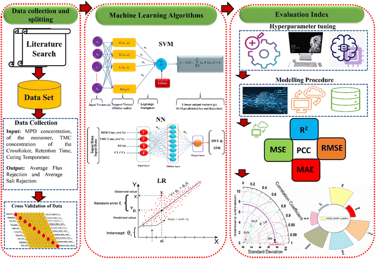
In this study, the methodology focuses on the data-driven approaches and pre-processing of experimental data related to thin-film composite polyamide membranes, which is essential for handling small datasets and includes steps such as normalization and outlier removal. For this purpose, data-driven regression algorithms, including SVM, NN, LR, and MLR, are implemented to model and optimize desalination performance metrics like AWF and ASR (Fig. 1). The used data was Khorshidi et al.⁹ In addition, the experimental procedure can also be found in Khorshidi et al.⁹ obtained from the dataset includes MPD concentration (wt%), TMC concentration (wt%), reaction time (s) (RT), and curing temperature (°C) (CT), as the input variables with the antifouling water flux (AWF in LMH) and antifouling separation ratio (ASR in %) as the target variables. The model structure for predicting AWF and ASR involves two combinations, Combo-I and Combo-II. In both combinations, the input variables include RT, CT, MPD, and TMC in weight percentage. However, the present research presented the outcomes of Combo II using all four variables as inputs to simulate AWF and ASR. This structure clarifies how the operational parameters and chemical concentrations influence the performance metrics of the membranes, specifically AWF and ASR. The experimental data were divided into 70% training and 30% testing. The decision to divide the experimental data into 70% for training and 30% for testing is based on widely accepted practices in ML and statistical modeling, ensuring that the model developed is both robust and generalizable. The 70/30 split is a standard convention in the field, particularly for moderate-sized datasets, and has been proven to offer a good trade-off between model accuracy and validation precision.²⁵ By adopting this approach, the study adheres to best practices, ensuring that the ML models are reliable, accurate in their predictions, and applicable to real-world scenarios. This methodology ultimately enhances the credibility and robustness of the study's findings. The study introduces ensemble techniques that integrate the strengths of individual models to enhance prediction accuracy, using performance metrics such as Mean Absolute Error (MAE), Root Mean Squared Error (RMSE), and Nash-Sutcliffe Efficiency (NSE) for evaluation. Neural Networks are particularly used to analyze patterns that optimize membrane performance, with a feedback loop that iteratively refines the membrane fabrication parameters based on ML insights. The effectiveness of these parameters is then validated in practical desalination setups, ensuring that the ML-driven approach significantly enhances both the efficiency and sustainability of the desalination process.

Fig. 1 Proposed schematic modelling flowchart.

Theoretical foundations of the basic models

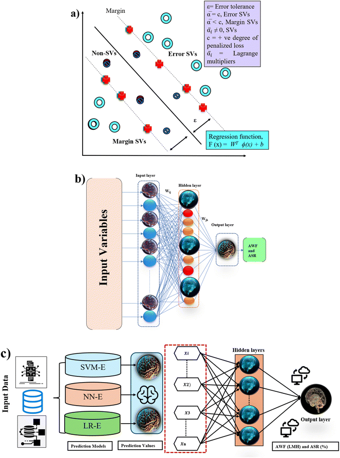
In ML and statistical modeling, SVM, NN (Fig. 2a and b), LR, and MLR offer a distinct toolkit for tackling a wide range of data analysis challenges. LR and MLR provide the foundations for understanding linear relationships between variables, with LR focusing on single-variable prediction and MLR extending to multiple predictors, both crucial for forecasting and interpreting the impact of variables on outcomes.²⁶ SVM advances into more sophisticated territory, excelling in classification and regression tasks within high-dimensional spaces by maximizing the margin between class boundaries, and effectively handling linear and non-linear data through kernel functions.^13,27 NN, inspired by the human brain neural structure, stands out for its ability to learn and model complex patterns across various applications, from image recognition to natural language processing, through layers of interconnected nodes.^28,29 These models span from simple to complex, offering tailored approaches to deciphering relationships in data.

Fig. 2 Fundamental architecture of (a) SVM, (b) NN and (c) ensemble learning.

The theory behind ensemble learning, particularly with neural networks, advances combining the outputs of multiple models to enhance predictive performance beyond what is achievable by any single model (Fig. 2c). This improvement stems from leveraging the diversity among models achieved through variations in training data subsets, initialization parameters, or architecture to reduce bias and variance in predictions.³⁰ By aggregating individual predictions using methods like averaging, weighted averaging, or voting, ensembles can capture a broader representation of the data distribution, mitigating overfitting and enhancing generalization to unseen data.^31–34 Although this approach offers significant benefits in accuracy and robustness, it also requires careful management of the trade-off between computational costs and performance gains, as training and deploying multiple models inherently demand more resources. Nonetheless, the strategic use of neural network ensembles remains a powerful technique for boosting the reliability and efficacy of predictive modeling across diverse applications.³³

Performance criteria

In evaluating the performance of predictive models, various criteria offer insights into accuracy, fit, and error, each with its unique theoretical foundation.^35–38 The performance of desalination membranes is critically assessed through specific criteria that include AWF and ASR. These metrics are essential for evaluating the efficiency and effectiveness of membrane technology in removing salt from seawater. Optimizing these performance indicators is fundamental to improving desalination processes. In addition, the precision of these measurements is often quantified using statistical metrics which help in assessing the accuracy of predictive models used in membrane design and operation. Such comprehensive evaluation ensures that enhancements in membrane technology lead to more sustainable and effective desalination solutions.

For instance, R-squared (R²) quantifies the variance explained by the model, serving as a gauge for goodness of fit, whereas the Pearson correlation coefficient (PCC) assesses the linear relationship between observed and predicted values. Mean squared error (MSE) and root mean squared error (RMSE) measure the average of the squared errors and the square root of these averages, respectively, reflecting the magnitude of prediction errors; both are sensitive to outliers, with RMSE being more commonly used due to its units being the same as those of the dependent variable. Mean Absolute Error (MAE) and Mean Absolute Percentage Error (MAPE) provide an understanding of average prediction error in absolute terms and as a percentage, making MAE straightforward to interpret and MAPE particularly useful for relative comparison across different scales. Percent Bias (PBIAS) evaluates the tendency of the predictions to be higher or lower than their actual values, indicating a model bias towards over or underestimation. Collectively, these metrics furnish a comprehensive toolkit for model evaluation, enabling the identification of models that best capture the underlying data patterns while balancing the trade-offs between simplicity, interpretability, and predictive accuracy.

Results and discussion

Hyperparameter tuning

It is important to note that hyperparameter tuning is essential for optimizing model performance by carefully adjusting parameters like learning rate, regularization, and network architecture. This process helps to balance accuracy, efficiency, and generalization, leading to more reliable and effective predictive models. The kernel type (RBF) and parameters like C and Gamma for the SVM model were optimized using grid search. This ensures the model efficiently handles the high-dimensional feature space typical of membrane performance data while balancing accuracy with computational efficiency. The NN model's number of layers and neurons per layer was fine-tuned using random search, with a deeper architecture chosen to capture complex relationships in the data and adjustments made to the learning rate and batch size to ensure stable and efficient training. The LR and MLR models were manually tuned to avoid overfitting while ensuring stable learning, which is particularly important when dealing with small datasets or less complex data structures (Table 1). For the ensemble approaches (NN-E and LR-E), techniques like bagging and boosting were employed to leverage the strengths of individual models while reducing their weaknesses, such as variance in NN or bias in LR. Including this table and discussion will comprehensively address the hyperparameter optimization process, providing transparency and justifying the choices made during model development.

Table 1 Hyperparameter tuning and optimization method

Model	Hyperparameters	Values set	Optimization technique	Rationale for choice
SVM	Kernel type	RBF	Grid search	Chosen for its balance between computational efficiency and accuracy in high-dimensional spaces
	C	1.0	Grid search	Adjusted for regularization to avoid overfitting
	Gamma	0.1	Grid search	Optimized for influence of single training examples
NN	Number of layers	3	Random search	Sufficient depth to capture non-linear patterns in data without overfitting
	Neurons per layer	[64, 32, 16]	Random search	Layer sizes decrease to allow for complex feature extraction followed by fine-tuning
	Learning rate	0.01	Random search	Set to balance between convergence speed and avoidance of local minima
	Batch size	32	Random search	Chosen for computational efficiency and stability during training
LR	Regularization	L^2	Manual tuning	L^2 regularization to penalize large coefficients, preventing overfitting
	Learning rate	0.001	Manual tuning	Small value chosen to ensure gradual learning and stable convergence
MLR	Coefficient estimation	Ordinary least squares	—	Default method for minimizing the residual sum of squares

---

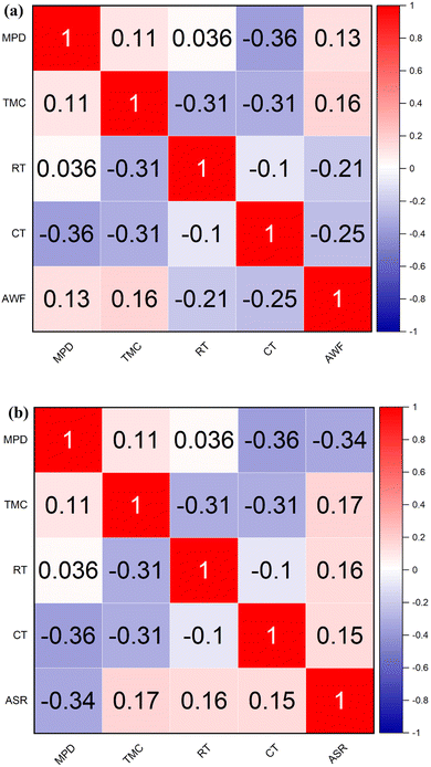
The results of implementing data-driven algorithms and ensemble techniques demonstrated significant improvements in predicting and optimizing the performance metrics of TFC polyamide membranes used in desalination processes. The dependency matrix from the study highlights that TMC concentration positively influences both target variables, antifouling AWF and antifouling ASR, with correlation values of 0.1642 and 0.1665, respectively. It suggests that higher concentrations of TMC generally improve both the throughput and efficiency of the filtration process. On the other hand, MPD concentration has a mixed impact; it shows a weak positive correlation with AWF (0.1327) (Fig. 3a), indicating a slight increase in water flux, but a moderate negative correlation with ASR (−0.3383), suggesting that higher MPD concentrations might degrade the separation efficiency. Furthermore, RT and CT exhibit contrasting effects on the two target variables. Both variables negatively affect AWF, with correlations of −0.2106 for RT and −0.2522 for CT, implying that longer RT and higher CT reduce water flux through the membrane. However, they show slight positive correlations with ASR (0.1575 for RT and 0.1530 for CT), indicating that these conditions may slightly improve the separation ratio. This differential impact highlights the complexity of membrane operation conditions, where adjustments to process parameters can enhance one aspect of performance at the expense of another (see Fig. 3b).

Fig. 3 Correlation-based dependency analysis based on (a) AWF and (b) ASR.

It is well known that understanding statistical parameters in modeling, such as mean, variance, skewness, and kurtosis, is crucial because it offers insights into data quality, reveals distribution characteristics, and helps in selecting appropriate modelling techniques.^39,40 It also guides preprocessing steps like normalization to improve model accuracy and predictability. Furthermore, knowing data distribution aids in choosing robust statistical tests and models, which is especially important when data is skewed or has outliers. Ultimately, this foundational understanding supports informed decision-making in experimental design and process optimization, leading to more effective and accurate outcomes.⁴¹ For this purpose, Table 2 presents descriptive statistics for antifouling AWF and ASR, alongside input variables MPD concentration, TMC concentration, RT, and CT. The mean values for all variables are consistent across both target metrics, with MPD and TMC concentrations showing controlled low variability. At the same time, RT and CT exhibit higher variability and extreme values, as indicated by their high kurtosis (11.000) and positive skewness. AWF and ASR differ significantly in their distribution characteristics; AWF has a higher standard deviation (30.360) and sample variance (921.734) compared to ASR (SD: 7.486, Variance: 56.047), along with a positive skewness (1.701) compared to ASR negative skewness (−3.020), suggesting more spread and a tail towards higher values in AWF. The minimum and maximum ranges (AWF: 15.300 LMH to 110.500 LMH, ASR: 72.100% to 97.600%) further underscore the extent of variability, particularly in AWF, which could be sensitive to experimental conditions or specific operational settings that favor certain ranges, indicating the need for careful analysis and interpretation of these measurements in related studies.

Table 2 Descriptive statistic for AWF and ASR target variables and other input variables

AWF	MPD	TMC	RT	CT	AWF
Mean	1.909	0.232	16.364	57.727	38.682
SD	0.831	0.087	4.523	9.045	30.360
Sample variance	0.691	0.008	20.455	81.818	921.734
Kurtosis	−1.485	−1.621	11.000	11.000	2.363
Skewness	0.190	0.409	3.317	3.317	1.701
Minimum	1.000	0.150	15.000	55.000	15.300
Maximum	3.000	0.350	30.000	85.000	110.500

---

ASR	MPD	TMC	RT	CT	ASR
Mean	1.909	0.232	16.364	57.727	94.045
SD	0.831	0.087	4.523	9.045	7.486
Sample variance	0.691	0.008	20.455	81.818	56.047
Kurtosis	−1.485	−1.621	11.000	11.000	9.413
Skewness	0.190	0.409	3.317	3.317	−3.020
Minimum	1.000	0.150	15.000	55.000	72.100
Maximum	3.000	0.350	30.000	85.000	97.600

---

Predictive results and comparison

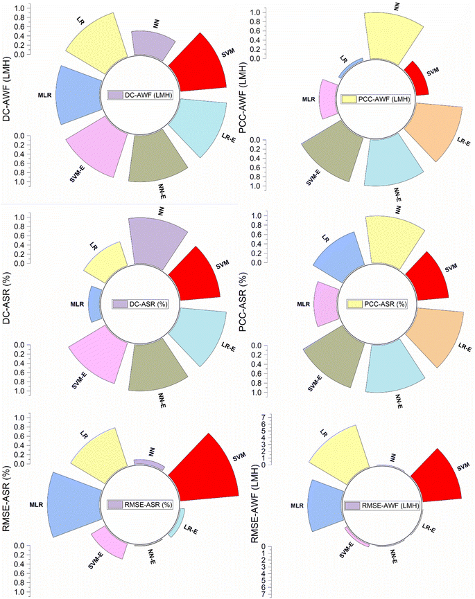
The predictive insight is also presented in Table 3, which provides performance validation results for different ML algorithms applied to optimize TFC polyamide membranes for desalination. From the table of AWF, the NN model exhibits the best performance with the lowest MAE (0.001) and RMSE (0.0111), indicating highly accurate predictions. Similarly, SVR and LR obtained average MAE and RMSE values with SVM-MAE = 0.573 and RMSE = 5.6948, while LR-MAE = 0.487 and RMSE = 6.5068. The MLR has a higher MAE (0.6379) than SVM but a lower RMSE (4.9084) than both SVM and LR, which suggests that MLR has a lower spread of errors than SVM and LR but not necessarily lower individual errors. However, for ASR, the NN outperforms the other models with the lowest MAE (0.0107) and RMSE (0.0982), which indicates its superior prediction capability in terms of accuracy. While SVM follows with an MAE of 0.0823 and an RMSE of 1.2664, demonstrating reasonable prediction accuracy. LR shows less accuracy than SVM with a higher MAE of 0.1269 and RMSE of 0.8713. MLR has the highest MAE (0.1434) and RMSE (1.1252) among the models for ASR prediction, suggesting it is the least accurate in this context. The NN exceptional performance could be due to its ability to capture complex non-linear relationships that might be present in the data. It is important to note that such perfect scores might also indicate overfitting, although this is not directly observable from the metrics provided. The relatively poorer performance of MLR indicates that the relationships between the variables in the dataset might be too complex for a linear model to capture accurately.^42–44 Based on the quantitative results, NN would be the preferred model for predicting both AWF and ASR in this context (see, Fig. 4). However, one should also consider the complexity of the model and the risk of overfitting, especially when dealing with small datasets. Ensemble techniques, as mentioned in the study aim, might help in improving the robustness of the predictions by combining the strengths of individual models.

Table 3 Performance validation results for prediction of AWF and ASR

	R^2	PCC	MSE	MAPE	MAE	PBIAS	RMSE
AWF (LMH)
SVM	0.8219	0.2697	32.4305	1.0137	0.5730	0.5644	5.6948
NN	1.0000	1.0000	0.0001	0.0039	0.0010	0.0000	0.0111
LR	0.7278	0.0596	42.3386	0.7865	0.4870	0.3872	6.5068
MLR	0.1218	0.3489	24.0926	1.9257	0.6379	0.0000	4.9084
ASR (%)
SVM	0.8613	0.6734	1.6036	0.1099	0.0823	−0.0245	1.2664
NN	0.9942	0.9971	0.0096	0.0113	0.0107	0.0000	0.0982
LR	0.5449	0.7381	0.7592	0.1413	0.1269	0.0000	0.8713
MLR	0.2410	0.4909	1.2661	0.1655	0.1434	0.0000	1.1252

---

Fig. 4 Predictive fitting based on error and goodness-of-fit utilizing radial diagram.

For the predictive approach, NN and MLR achieved a PBIAS of 0 for both AWF and ASR, indicating an unbiased prediction for these crucial desalination parameters. In contrast, SVM exhibited a PBIAS of 0.5644 for AWF, suggesting a slight underestimation, and −0.0245 for ASR, indicating a minor overestimation. LR, with a PBIAS of 0.3872 for AWF, also showed a tendency to underestimate but did not provide a PBIAS value for ASR. While NN demonstrated superior accuracy and lack of bias, ensuring that these findings are not a result of overfitting is vital for their application in desalination process optimization. Although MLR displayed no bias, its higher predictive errors imply it might be less dependable. Any bias or error in the model predictions can significantly impact the environmental outcomes of the desalination process by causing either an overuse or underuse of resources, which can lead to increased energy consumption and an escalated environmental footprint. Therefore, it is imperative for the selected model to not only exhibit minimal predictive error but also to faithfully represent actual operations to ensure that the desalination process is environmentally sustainable.

However, the predictive modelling using AWF and ASF was evaluated using a violin diagram. It is important to note that violin plots are essential for visually analyzing the distribution and relationships of variables such as MPD, TMC, RT, CT, and operating conditions, enabling the identification of influential factors and validation of predictive models in predicting desalination flux and rejection outcomes (see, Fig. 5). In assessing the performance of ML models for predicting AWF and ASR in desalination, the R² reveals the proportion of variance each model captures from the dependent variable. For AWF, the NN model achieved a perfect R² score of 1, indicating a model that accounts for all variance in the dataset, followed by the SVM with an R² of 0.8219, signifying a robust model fit. The LR recorded an R² of 0.7278, showing a good but lesser fit compared to SVM, while MLR lagged with an R² of 0.1218, suggesting a poor model fit. When predicting ASR, the NN model remained superior with an R² = 0.9942, closely approaching a perfect fit. The SVM model also performed well with an R² = 0.8613, whereas the LR model's fit was moderate with an R² = 0.5449, and the MLR model again showed a weak fit with an R² = 0.241. These R² values are crucial for evaluating the model's predictive quality in desalination, as a high R² corresponds to more accurate predictions of membrane performance, which is fundamental to the efficiency and sustainability of water treatment processes. The numerical outcomes of AWF using the NN model showed a 21.67% increase over the SVM, a 37.40% increase over LR, and a substantial 721.02% increase over MLR. Similarly, for ASR, the increases were 15.43% over SVM, a significant 82.46% over LR, and a remarkable 312.53% over MLR. These increases underscore the NN model enhanced predictive accuracy for both key performance indicators in the domain of desalination.

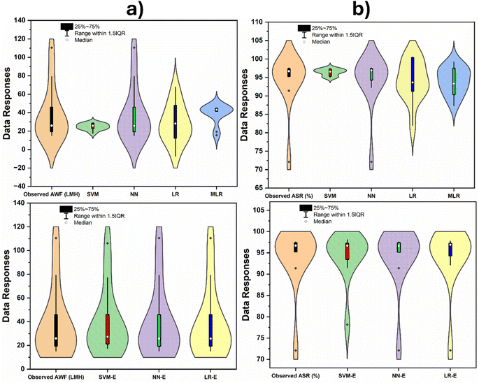Fig. 5 Spread of predictive results based between the observed and simulated AWF (a) and ASR (b) using violin diagram.

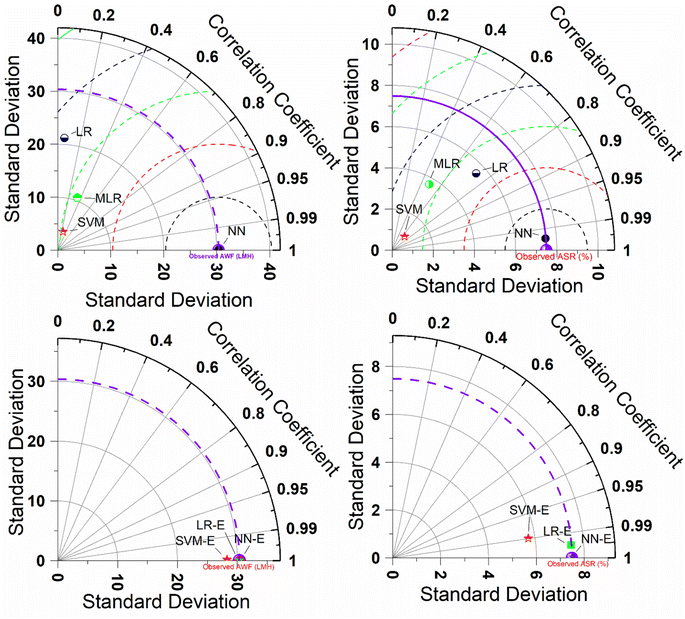
Further understanding of violin plots comparing the predictive performance of various ML models against observed data for AWF and ASR. Violin plots are useful for displaying the distribution of data and its probability density. The left side of the figure shows the results for AWF, while the right side is for ASR. The plots for each model display the range of predicted values, with thicker sections representing a higher density of data points. The black horizontal line inside each violin represents the interquartile range (25–75%), with the black dot indicating the median of the predictions. The range within 1.5 times the interquartile range (IQR) is indicated by the black lines extending from the interquartile range, showing the spread of the majority of the data. For AWF (left plots), the observed data has a narrow interquartile range and a higher median compared to the predictions by the SVM and LR models, which show a wider distribution of responses, indicating variability in their predictions. The NN model has a very tight distribution, closely matching the observed data, suggesting high accuracy and precision. The MLR shows a broad distribution, suggesting lower precision. Similarly, for ASR (right plots), the observed data shows a slightly broader distribution compared to AWF but still maintains a higher median than most predictive models. The SVM and LR models show wide distributions, indicating variability and less precision in predictions. The NN has a narrow distribution for ASR as well, closely aligning with the observed data, which implies accuracy and consistency in its predictions. The MLR again shows a wide distribution. The lower plots are labelled with an E suffix (SVM-E, NN-E, LR-E), which could indicate an ensemble approach. These ensemble models generally show narrower distributions compared to their non-ensemble counterparts, especially for SVM-E and NN-E, suggesting that ensemble improves prediction accuracy and consistency. In general, for both AWF and ASR, the NN model, and potentially its ensemble version, provides the closest match to the observed data, indicating it may be the most reliable for predicting desalination membrane performance. The use of ensembles appears to refine the predictions, potentially leading to more precise and accurate models, which is crucial for designing efficient and environmentally friendly desalination processes. The predictive skills can also be proved using 2-dimensional (2D) Taylor diagram as indicated in Fig. 6.

Fig. 6 2D-Taylor diagram to show the comparison of the models in term of several indicators.

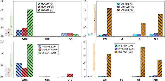
In Table 4, the ensemble models show high NSE values for the prediction of AWF and ASR, indicative of excellent model performance. Specifically, for AWF, the SVM-E exhibits an NSE of 0.994, suggesting a very close match to the observed data, while both the NN-E and the LR-E achieve a perfect NSE of 1, reflecting predictions that perfectly match the observed measurements. For ASR predictions, SVM-E NSE of 0.8741, although lower than for AWF, still indicates a good predictive match, whereas NN-E again achieves a perfect NSE of 1, and LR-E is nearly perfect at 0.9947. These high NSE values signal the robustness of the ensemble models in capturing the true variance of the observed data, minimizing prediction noise. The exceptional performance of these ensemble models in desalination modeling has a direct environmental impact, as accurate predictions of AWF and ASR are critical for optimizing the desalination process, leading to significant energy and resource savings, more efficient water usage, reduced waste, and a lower environmental footprint for water treatment facilities. This in turn, minimizes the ecological footprint of desalination plants by ensuring they operate at peak performance, reducing waste and the potential for excessive chemical and energy use, which are pivotal considerations in the sustainable management of water resources. In Table 3, the MAPE values for ensemble ML models provide insights into the accuracy of predictions for desalination process parameters. For AWF, the SVM-E shows a MAPE of 0.2227 (22.27%), while the NN-E and the LR-E both demonstrate extraordinarily low MAPE values of 0.004 (0.4%) and 0.0039 (0.39%), respectively. In the case of Average Salt Rejection (ASR), SVM-E has a MAPE of 0.0378 (3.78%), NN-E achieves a MAPE of 0.0013 (0.13%), and LR-E presents a MAPE of 0.014 (1.4%) (see, Fig. 7). These low MAPE values, particularly for NN-E and LR-E, indicate a high level of precision in predictive modelling, which is environmentally beneficial for desalination operations.

Table 4 Ensemble validation results for prediction of AWF and ASR

	R^2	NSE	PCC	MSE	MAPE	MAE	PBIAS	RMSE
AWF (LMH)
SVM-E	0.9948	0.9940	1.0000	0.1423	0.2227	0.0597	−0.0171	0.3772
NN-E	1.0000	1.0000	1.0000	0.0001	0.0040	0.0010	0.0000	0.0111
LR-E	1.0000	1.0000	1.0000	0.0001	0.0039	0.0010	0.0000	0.0111
ASR (%)
	R^2	NSE	PCC	MSE	MAPE	MAE	PBIAS	RMSE
SVM-E	0.9265	0.8741	0.9898	0.1226	0.0378	0.0303	−0.0036	0.3501
NN-E	1.0000	1.0000	1.0000	0.0001	0.0013	0.0013	0.0000	0.0089
LR-E	0.9947	0.9947	0.9974	0.0088	0.0140	0.0133	0.0000	0.0936

---

Fig. 7 Comparison between single and improved error ensemble for different models.

In Table 4, for AWF predictions, the SVM-E reports an RMSE of 0.3772 and an MAE of 0.0597, while both the NN-E and the LR-E exhibit remarkably low values with an RMSE of 0.0111 and an MAE of 0.001. As for ASR predictions, SVM-E demonstrates an RMSE of 0.3501 and an MAE of 0.0303, which, though moderate, are higher than the values for NN-E and LR-E. NN-E shows an exceptionally low RMSE of 0.0089 and an MAE of 0.0013, suggesting an extremely high accuracy in predictions. LR-E also performs well with an RMSE of 0.0936 and an MAE of 0.0133, indicating a high degree of precision, albeit slightly less than that of NN-E. These RMSE and MAE values emphasize the robustness of NN-E and LR-E in modelling, with NN-E being particularly notable for its precision, which is crucial for optimizing desalination processes, leading to environmental benefits such as reduced energy consumption, and minimized waste. The predictive comparison between Tables 3 and 4 reveals that ensemble models substantially enhance predictive accuracy for desalination processes. In Table 4, individual models, with NN performing the best, achieve an MAE of 0.001 and an RMSE of 0.0111 for AWF, and an MAE of 0.0107 and RMSE of 0.0982 for ASR. However, Table 4 ensemble models outshine these figures, with the NN-E and -E for AWF both yielding an MAE of 0.001 and an RMSE of 0.0111, while the SVM-E records a slightly higher MAE of 0.0597 and RMSE of 0.3772. For ASR, the NN-E impressively lowers the MAE to 0.0013 and the RMSE to 0.0089, and the LR-E follows closely with an MAE of 0.0133 and an RMSE of 0.0936, with the SVM-E improving to an MAE of 0.0303 and an RMSE of 0.3501. These reductions in error metrics underscore the effectiveness of ensemble methods in increasing the precision and reliability of predictive modeling for desalination, leading to environmentally and economically optimized operations through better resource management and reduced waste. Generally, the ensemble models, particularly those integrating NN and LR, exhibited enhanced predictive accuracy for AWF and ASR, outperforming individual algorithm-based models. This superiority is evidenced by lower MAE and RMSE values, alongside near-perfect NSE scores, highlighting the effectiveness of the ensemble approach in capturing complex nonlinear relationships within the data.

SHAP analysis results

It is essential to note that SHAP analysis provides a clear and interpretable quantification of each feature's contribution to a model's predictions, enhancing transparency and understanding of complex machine learning models.

Global interpretability

The global bar plot (Fig. 8) ranks the features based on their average SHAP values, which represent their overall contribution to the model's predictions across the dataset. For the ASR, MDP shows the highest average SHAP value of 0.35, indicating that it is the most influential feature in determining the ASR. This suggests that variations in MDP can lead to significant changes in the model's output, making it a critical parameter for optimizing membrane performance. In comparison, TMC for AWF has an average SHAP value of 0.28, making it a key driver for water flux in the desalination process. These SHAP values provide a clear quantification of the importance of each feature, guiding the prioritization of features during model tuning and membrane design. In contrast, the feature with an average SHAP value of 0.10, has a relatively minor impact, suggesting that while it contributes to the predictions, its role is less significant compared to MDP and TMC. Likewise, the local bar plot offers a more granular view by showing the SHAP values for individual predictions, illustrating how specific features influence the model's output in particular instances. For example, in one instance predicting AWF, MDP has a SHAP value of 0.22, indicating a strong positive contribution to the water flux prediction for that particular data point. This means that MDP is pushing the model's prediction upward for that instance. On the other hand, CT might show a SHAP value of −0.15 for the same instance, indicating that it negatively impacts the predicted AWF, reducing the model's output for that data point. This type of analysis is particularly useful for identifying and understanding the specific conditions or interactions under which certain features exert a strong influence, either positively or negatively, on the prediction.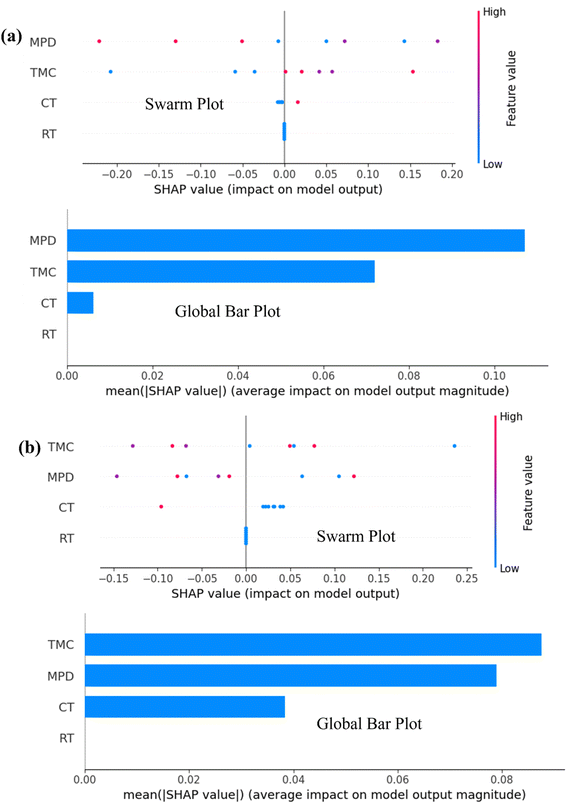

Fig. 8 SHAP results for global interpretability using Global bar plot and swarm plot for (a) ASR and (b) AWF.

Local interpretability

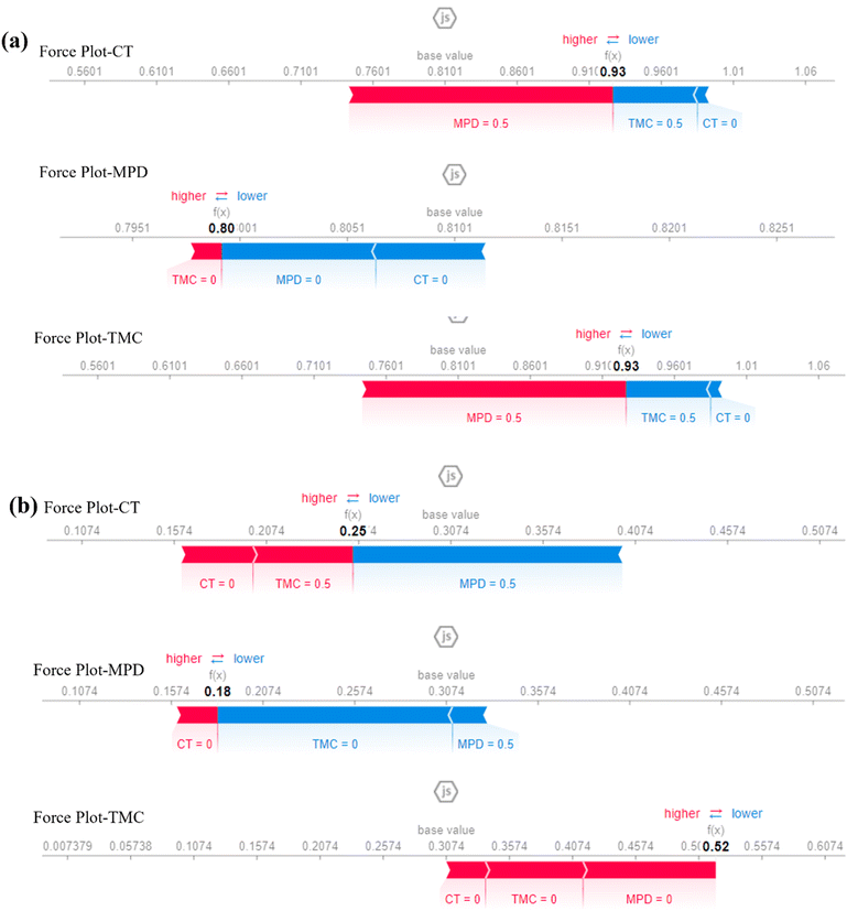
Furthermore, the local bar plot (Fig. 9) might reveal that RT has a high positive SHAP value of 0.30 in a specific ASR prediction, indicating that it significantly boosts the salt rejection in that case. This insight could be crucial for identifying specific scenarios or membrane conditions that enhance performance, which could inform further experimental investigations or targeted improvements in membrane design. The SHAP analysis, through both global and local bar plots, offers a comprehensive understanding of feature importance in the model's predictions for AWF and ASR. The global analysis highlights which features are generally most influential across all predictions, with MDP and TMC being particularly critical for ASR and AWF, respectively. The local analysis provides detailed insights into how these features affect individual predictions, helping to identify specific cases where certain features have an outsized influence. Generally, the SHAP force plot provided for the features MDP, TMC, and CT based on the ASR output offers a detailed visualization of how each feature contributes to a specific prediction by either increasing or decreasing the predicted value relative to a baseline, typically the mean prediction. This plot is particularly useful for understanding how individual features push the model's prediction higher or lower in specific instances (Fig. 9). For MDP, if the force plot shows a significant contribution to a higher ASR prediction, it indicates a positive correlation with better salt rejection in that specific case. The magnitude of this contribution is visually represented by the length of the arrow or bar associated with MDP; a longer arrow pointing toward a higher prediction value suggests that MDP is a major driver of the model's prediction. TMC's contribution might vary depending on the scenario; if the force plot shows TMC pulling the prediction down, it suggests a negative impact on ASR, possibly due to suboptimal conditions or interactions with other features. CT might also either push the prediction up or pull it down, depending on how it interacts with MDP and TMC in the instance.

Fig. 9 SHAP for model's Local bar plot interpretability for force plot (a) ASR and (B) AWF.

For example, if CT reduces the predicted ASR, it might indicate that higher CT values are associated with lower salt rejection efficiency under these conditions. The force plot thus provides a detailed, instance-specific breakdown of how MDP, TMC, and CT contribute to the final prediction, allowing us to see the dynamics between these features in a clear and interpretable way. If MDP shows the strongest positive contribution while TMC and CT have smaller or negative contributions, optimizing MDP could be more critical for enhancing ASR in this specific case. The force SHAP plot offers a granular view of how MDP, TMC, and CT interact to affect the model's prediction of ASR in individual cases, providing insights that can inform targeted improvements in membrane design or operational conditions (Fig. 9). This detailed interpretability is crucial for understanding the complex relationships within the model and ensuring that the predictions are both reliable and actionable.

Conclusion

This research explained the profound impact of advanced ML techniques and their ensembled techniques on the desalination industry, a field where precision and efficiency are not just beneficial but essential. By modelling AWF and ASR, we addressed the potential for significant environmental and operational enhancements in desalination practices. The individual ML models evaluated SVM, NN, LR, and MLR provided a foundational understanding of the data complexity. NN demonstrated exemplary predictive power with a perfect R² value of 1 for both AWF and ASR, alongside the lowest MAE and RMSE, marking a significant stride in predictive capabilities. However, the ensemble models took accuracy and reliability to new heights. With near-perfect NSE values, they outperformed individual models, illustrating that an integrative approach to predictive analytics can surpass the sum of its parts. For AWF, both NN-E and LR-E maintained an MAE and RMSE of 0.001 and 0.0111, respectively, while for ASR, NN-E reduced the MAE further to 0.0013 and the RMSE to a remarkably low 0.0089. Such accurate predictions imply enhanced RO membrane desalination by optimizing monomer concentration and interfacial conditions, thereby improving AWF and ASR. The complexity of different monomer structures limits sparse dataset ability to generalize across diverse RO membrane types effectively. Incorporating deep learning across a wide range of monomers, emerging neuro-intelligent ensemble models will offer the potential to optimize interfacial conditions, significantly enhance the performance of polyamide RO membranes, and deepen our understanding of monomer interaction. This study provides insights into improving the real-time efficacy of RO membrane performance, thereby contributing to global water scarcity mitigation through cost reduction. This study serves as a foundation for the integration of membrane technology and machine learning, with the goal of optimizing desalination processes and maximizing freshwater production.

Abbreviations

AI	Artificial intelligence
ANN	Artificial neural networks
ASR	Average salt rejection
AWF	Average water flux
CT	Curing temperature
D-ANN	Dual-output neural network
DNN	Deep learning neural network
GA	Genetic algorithms
GBM	Gradient boosting machines
LMH	Liters per meter square per hour
LR	Linear regression
LR-E	Linear regression ensemble
MAE	Mean absolute error
MAPE	Mean absolute percentage error
MGPR	Matern Gaussian process regression
ML	Machine learning
MLR	Multivariate linear regression
MPD	m-Phenylenediamine
MSE	Mean squared error
NF	Nanofiltration
NN	Neural networks
NN-E	Neural networks ensemble
NSE	Nash-Sutcliffe efficiency
PBIAS	Percent bias
PCC	Pearson correlation coefficient
R^2	R-squared
RMSE	Root mean squared error
RO	Reverse osmosis
RT	Reaction time
SD	Standard deviation
SDG	Sustainable development goal
SHAP	Shapley additive explanations
SVM	Support vector machine
SVM-E	Support vector machine ensemble
TFC	Thin-film composite
TMC	Trimesoyl chloride
XAI	Explainable artificial intelligence

Data availability

Data and articles, including all descriptions of data types, are available at (https://rsc.66557.net/en/content/articlelanding/2015/ra/c5ra08317f).

Conflicts of interest

There are no conflicts to declare.

References

1. L. Fu, X. Zhou, L. Deng, M. Liao, S. Chen, H. Wang and L. Wang, Desalination, 2023, 550, 116362.
2. X. Lu and M. Elimelech, Chem. Soc. Rev., 2021, 50, 6290–6307.
3. UN DESA, SDGs Report 2023, 2023.
4. S. Fayyaz, S. Khadem Masjedi, A. Kazemi, E. Khaki, M. Moeinaddini and S. Irving Olsen, J. Cleaner Prod., 2023, 382, 135299.
5. R. R. Choudhury, J. M. Gohil, S. Mohanty and S. K. Nayak, J. Mater. Chem. A, 2018, 6, 313–333.
6. X. Sun, L. Duan, Z. Liu, Q. Gao, J. Liu and D. Zhang, J. Environ. Manage., 2024, 349, 119634.
7. R. H. Hailemariam, Y. C. Woo, M. M. Damtie, B. C. Kim, K. D. Park and J. S. Choi, Adv. Colloid Interface Sci., 2020, 276, 102100.
8. Y. Chen, Q. Jason Niu, Y. Hou and H. Sun, Sep. Purif. Technol., 2024, 330, 125282.
9. B. Khorshidi, T. Thundat, B. A. Fleck and M. Sadrzadeh, RSC Adv., 2015, 5, 54985–54997.
10. X. Li, Z. Wang, X. Han, Y. Liu, C. Wang, F. Yan and J. Wang, J. Membr. Sci., 2021, 640, 119765.
11. T. Yang, C. F. Wan, J. Zhang, C. Gudipati and T. S. Chung, J. Membr. Sci., 2021, 626, 119187.
12. J. Usman, U. Baig, S. I. Abba, F. A. Alharthi, C. M. Fellows, A. Waheed and I. H. Aljundi, J. Environ. Chem. Eng., 2024, 12, 112569.
13. N. Baig, J. Usman, S. I. Abba, M. Benaafi and I. H. Aljundi, J. Cleaner Prod., 2023, 138193.
14. H. Li, B. Zeng, J. Tuo, Y. Wang, G. P. Sheng and Y. Wang, J. Membr. Sci., 2024, 692, 122320.
15. T. Zhu, Y. Zhang, C. Tao, W. Chen and H. Cheng, Sci. Total Environ., 2023, 857, 159348.
16. M. Talhami, T. Wakjira, T. Alomar, S. Fouladi, F. Fezouni, U. Ebead, A. Altaee, M. AL-Ejji, P. Das and A. H. Hawari, J. Water Process Eng., 2024, 57, 104633.
17. S. L. Mousavi and S. M. Sajjadi, RSC Adv., 2023, 13, 23754–23771.
18. P. Dansawad, Y. Li, Y. Li, J. Zhang, S. You, W. Li and S. Yi, Adv. Membr., 2023, 3, 100072.
19. C. S. H. Yeo, Q. Xie, X. Wang and S. Zhang, J. Membr. Sci., 2020, 606, 118135.
20. A. Mohammed, H. Alshraideh and F. Alsuwaidi, Desalination, 2024, 574, 117253.
21. T. Bonny, M. Kashkash and F. Ahmed, Desalination, 2022, 522, 115443.
22. H. Li, B. Zeng, T. Qiu, W. Huang, Y. Wang, G. P. Sheng and Y. Wang, J. Membr. Sci., 2023, 687, 122093.
23. Z. Zhang, Y. Luo, H. Peng, Y. Chen, R. Z. Liao and Q. Zhao, J. Membr. Sci., 2021, 620, 118910.
24. A. Tayyebi, A. S. Alshami, E. Tayyebi, C. Buelke, M. J. Talukder, N. Ismail, A. Al-Goraee, Z. Rabiei and X. Yu, Desalination, 2024, 579, 117502.
25. A. M. Jibrin, M. Al-Suwaiyan, A. Aldrees, S. Dan’azumi, J. Usman, S. I. Abba, M. A. Yassin, M. Scholz and S. S. Sammen, Sci. Rep., 2024, 14, 1–16.
26. A. Gbadamosi, H. Adamu, J. Usman, A. G. Usman, M. M. Jibril, B. A. Salami, S. L. Gbadamosi, L. O. Oyedele and S. I. Abba, Int. J. Hydrogen Energy, 2024, 50, 1326–1337.
27. J. Usman, S. I. Abba, N. Baig, N. Abu-Zahra, S. W. Hasan and I. H. Aljundi, ACS Appl. Mater. Interfaces, 2024, 16(13), 16271–16289.
28. N. Baig, S. I. Abba, J. Usman, M. Benaafi and I. H. Aljundi, Environ. Sci. Adv., 2023, 2, 1446–1459.
29. J. Usman, S. I. Abba, N. B. Ishola, T. El-Badawy, H. Adamu, A. Gbadamosi, B. A. Salami, A. G. Usman, M. Benaafi, M. H. D. Othman and I. H. Aljundi, Chem. Eng. Res. Des., 2023, 199, 33–48.
30. A. G. Usman, S. Işik, S. I. Abba and F. Meriçli, J. Sep. Sci., 2021, 44, 843–849.
31. F. A. B and S. Sadaoui, Multi-class Ensemble Learning, Springer International Publishing, 2019.
32. P. Ganguli and M. J. Reddy, Hydrol. Processes, 2013, 5009, 4989–5009.
33. T. G. Dietterich, Ensemble methods in machine learning, in, International Workshop on Multiple Classifier Models, 1996, vol. 12, pp. 1–15, (265–275),  DOI:10.1007/3-540-45014-9_1.
34. S. Tewari and U. D. Dwivedi, Comput. Ind. Eng., 2019, 128, 937–947.
35. S. K. Bhagat, T. Tiyasha, A. Kumar, T. Malik, A. H. Jawad, K. M. Khedher, R. C. Deo and Z. M. Yaseen, J. Environ. Manage., 2022, 309, 114711.
36. J. S. Chou and D. K. Bui, Energy Build., 2014, 82, 437–446.
37. H. K. Balsora, A. Kartik, V. Dua, J. B. Joshi, G. Kataria, A. Sharma and A. G. Chakinala, J. Environ. Chem. Eng., 2022, 10, 108025.
38. V. Nourani, A. Molajou, H. Najafi and A. Danandeh, Mehr, 2019, 45–61.
39. M. Nishio and A. Arakawa, Genet., Sel., Evol., 2019, 51, 1–12.
40. E. Arandia, A. Ba, B. Eck and S. McKenna, J. Water Resour. Plan. Manag., 2016, 142, 04015067.
41. S. I. Abba, M. Benaafi and I. H. Aljundi, Desalination, 2023, 550, 116376.
42. H. U. Abdullahi, A. G. Usman, S. I. Abba and H. U. Abdullahi, Dutse J. Pure Appl. Sci., 2020, 6, 362–371.
43. M. A. Ghorbani, R. Khatibi, A. Goel, M. H. FazeliFard and A. Azani, Environ. Earth Sci., 2016, 75, 1–13.
44. S. Heddam, Environ. Monit. Assess., 2014, 186, 7837–7848.

---