Experimentally-based Fe-catalyzed ethene oligomerization machine learning model provides highly accurate prediction of propagation/termination selectivity

Abstract

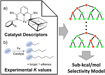
Linear α-olefins (1-alkenes) are critical comonomers for ethene copolymerization. A major impediment in the development of new homogeneous Fe catalysts for ethene oligomerization to produce comonomers and other important commercial products is the prediction of propagation versus termination rates that control the α-olefin distribution (e.g., 1-butene through 1-decene), which is often referred to as a K-value. Because the transition states for propagation versus termination are generally separated by less than a one kcal mol⁻¹ difference in energy, this selectivity cannot be accurately predicted by either DFT or wavefunction methods (even DLPNO-CCSD(T)). Therefore, we developed a sub-kcal mol⁻¹ accuracy machine learning model based on several hundred experimental selectivity values and straightforward 2D chemical and physical features that enables the prediction of α-olefin distribution K-values. As part of our model, we developed a new ad hoc feature that boosted the model performance. This machine learning model captures the effects of a broad range of ligand architectures and chemically nonintuitive trends in oligomerization selectivity. Our machine learning model was experimentally validated by prediction of a K-value for a new Fe phosphaneyl–pyridinyl–quinoline catalyst followed by experimental measurement that showed precise agreement. In addition to quantitative predictions, we demonstrate how this machine learning model can provide qualitative catalyst design using proximity of pairs type analysis.

---

Introduction

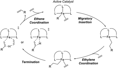
Linear α-olefins (i.e., 1-alkenes), specifically C₄ to C₁₈, are important chemical precursors used in the production of several relevant commodities such as polyethylene, plasticizers, lubricants, surfactants, and other materials.^1,2 The Shell Higher Olefin Process (SHOP) generates these α-olefins with a Ni catalyst, and Idemitsu and SABIC-Linde use Zr-based catalysts.^3–5 Chevron Phillips Chemical and INEOS operate processes based on triethylaluminum catalysts under high pressure and temperature (>175 °C).⁶ Fe-based catalysts are highly desirable due to the abundant, low-cost, and non-toxic nature of iron. Iron oligomerization catalysts generally display high reactivity, and enable significant diversity of ligand architectures that can be used to control reaction selectivity.^7–13 Perhaps the most prominent example of a molecular Fe catalyst for α-olefin production is the tridentate pyridine bisimine (PBI) Fe complex (I in Fig. 1a) reported by both Gibson⁸ and Small and Brookhart.^9,14 A major impediment in the design of novel Fe-based tridentate ethene oligomerization catalysts is the prediction of the α-olefin selectivity distribution. The chelating ligand framework has a major impact on the distribution ranging from C₄ to longer oligomers that are waxes (C₂₀₊).^15–20

Fig. 1 The general workflow involves combining 2D descriptors for Fe-imine type catalysts with experimental K-values to develop an accurate machine learning model (e.g. Random Forest type shown) to predict ethene oligomerization α-olefin selectivity. (a) Small and Brookhart's (PBI) Fe type catalysts and 2D descriptors to describe the aryl groups. (b) Overview of ethene oligomerization generating a distribution of α-olefins, which is quantitatively described by experimentally measured K-values.

The distribution of α-olefins produced is typically described as the K-value that is a measure of the selectivity for the rate of propagation versus the rate of termination during oligomerization (Scheme 1) and is defined as the oligomer fraction that propagates versus the total propagation and termination for a single ethene insertion step.^21–23 This value, which is mathematically described as a constant that is between 0 and 1, often shows small amounts of drift over the total product range, and is therefore generally reported for C₁₂/C₁₀ or C₁₄/C₁₂.²⁰ It has generally been established that propagation-termination selectivity is controlled by the energy difference between transition states for Fe-alkyl ethene insertion for propagation and termination by β-hydrogen transfer.^20,24–26 Importantly, based on experimentally reported K-values and statistical rate theory, the energy difference between these transition states is often less than 1 kcal mol⁻¹. Thus, predicting the K-values for ethene oligomerization is outside the reach of density functional theory (DFT) and generally outside the reach of CCSD(T) or DLPNO-CCSD(T) that can be applied to moderate to large size catalysts.^27,28 While energy scaling to magnify the energy differences between transition states can be applied, this approach generally cannot be applied to a large variety of catalysts in a predictable manner.²⁸ Therefore, we postulated that a machine learning based model built using experimental data and molecular structure features may provide the necessary sub-kcal mol⁻¹ accuracy to enable the prediction of K-values across a variety of ligand families. In addition to the model being based on experiments rather than DFT computed data, this type of approach has the advantage of no significant computational cost to predict the K-values of new possible ligands. Additionally, as we have previously shown for Cr ethene trimerization, machine learning models can provide key qualitative insights for further catalyst design.²⁹

Scheme 1 General catalytic cycle for tridentate Fe-catalyzed ethene oligomerization.

Here, we disclose the development and use of a machine learning model that enables prediction of a K-value within a mean absolute error of only 0.05, which is equivalent to an energy error of less than 0.15 kcal mol⁻¹ for transition-state/statistical-theory-based selectivity. This experimentally based machine learning model was developed using straightforward 2-dimensional (2D) molecular features as well as a newly created feature that describes the ligand arms (Fig. 1a). This machine learning model captures the effects of a broad range of ligand architectures and replicates and predicts chemically nonintuitive trends in oligomerization α-olefin selectivity. Validation of the machine learning model was then achieved by prediction and experimental measurement of a K-value for a new Fe phosphaneyl–pyridinyl–quinoline (PPQ) catalyst. In addition to quantitative prediction of K-values, we illustrate how this machine learning model can provide qualitative catalyst design using proximity of pairs analysis. Overall, this model provides a lynchpin for choosing new Fe ethene oligomerization catalysts to develop.

Machine learning model

Machine learning has become a highly popular and useful tool for predicting catalyst properties, especially for heterogeneous systems and solid-state materials.^30–33 Compared to heterogeneous catalysts and materials, there has been significantly less direct use and success of machine learning to design molecular, homogeneous transition metal catalysts, especially with post-prediction experimental realization. In most machine learning efforts, there is often a reliance on DFT calculated energies and properties.^34–37 Unfortunately, the use of DFT calculated energies can be severely problematic for selectivity that requires very high accuracy.

To aid in the design of new molecular Fe-based catalysts for ethene oligomerization, we targeted the development of a machine learning model built with experimental selectivity values and straightforward molecular descriptors (features) that do not rely on information generated from quantum-chemical calculations, such as atomic charges or vibrational frequencies. Sigman and others have previously demonstrated the power of using molecular descriptors to predict reactivity and selectivity in organic reactions.^38,39 Physical features such as reaction temperature and reagent loading are considered in our model. The selection of experimental data set, features, and machine learning algorithms are disclosed in detail below.

We constructed the experimental K(C₁₂/C₁₀) value data set using 116 unique polydentate (mostly tridentate) Fe catalysts, (see ESI Fig. S1† for a comprehensive list of catalyst structures).^{14,18,40–53}Fig. 2a shows a representative set examples of tridentate Fe catalysts bearing various ligand backbones featuring a diverse set of substituents on the ligand arms near the Fe center. This dataset includes N, O, and P direct coordination with the Fe metal center, and pyridine-bisimine, α-diimine, phenanthroline, iminopyridine, and other derivative ligands.

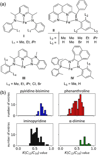Fig. 2 (a) Representative Fe ethene oligomerization catalysts used in our machine learning data set. (b) K(C₁₂/C₁₀) value distribution of the data set used in machine learning.

All 116 catalysts have at least one associated K-value, and several catalysts have more than one K-value corresponding to different reaction conditions (e.g., catalyst loading, cocatalyst identity, and reaction temperature). Our data set encompasses a total of 257 K-values for these 116 different catalysts. A few values were reported as K(C₁₄/C₁₂). These K(C₁₄/C₁₂) values were converted to K(C₁₂/C₁₀) values through the linear scaling:

K(C₁₂/C₁₀) = K(C₁₄/C₁₂) × 0.953 (1)

This scaling is justified based on experimental K-values for different carbon fractions (C₄–C₂₀) measured using a Fe pendant donor diimine (Fe(PDD)) catalyst.²⁰ Although this assumption might be less accurate for different catalyst ligands, the difference is expected to be within the error of the model. Fig. 2b plots the distribution of K(C₁₂/C₁₀) values. The values range from 0.25 to 0.89, and there is generally a smooth and continuous distribution of values between these endpoints.

Fourteen features were used to build the initial K-value machine learning model. We decided to include both chemical and physical features because, while we assumed the chemical features would be more important, we did not know if a quantitative machine learning model was possible to develop without physical features. Therefore, we began by using six physical features and eight molecular features. The six physical features correspond to reaction conditions including catalyst loading, co-catalyst loading, co-catalyst type, ethene pressure, reaction temperature, and time.

Seven of the eight molecular features are 2D features generated using the MordRed⁵⁸ and the RDkit⁵⁹ program based on structures represented in the simplified molecular-input line-entry system (SMILES) format (Table 1). These seven features can be categorized into two groups. Group I, including AMID_N and Xc-5dv, serves to identify ligand structures. Information regarding atomic connectivity and the sterics of the ligand are embedded within group A features (see the ESI† for more information). Group B features take into consideration ligand electronic properties in addition to topologies, hydrophilicity (SlogP-VSA1 and SlogP-VSA2), polarizability (SMR-VSA7), and electronegativities (SdssC and SaaaC).

Table 1 Descriptions of seven 2D molecular features as used in the machine learning model for K(C₁₂/C₁₀) value predictions

	Description
AMID_N^54	• Averaged molecular ID on N atoms; considers general structure near nitrogen atoms
Xc-5dv^55	• Valence 5th order cluster Chi index; considers bonding and valence electrons
SlogP-VSA1, SlogP-VSA2 (ref. 56)	• Subdivided surface area descriptor based on atomic log P (i.e., octanol/water partition coefficient) and estimated accessible van der Waals surface area; SlogP-VSA1 considers atoms with higher estimated hydrophilicity than those of SlogP-VSA2
SMR-VSA7 (ref. 56)	• Subdivided surface area descriptor based on atomic contribution to total polarizability (i.e., molar refractivity) of the ligand and estimated accessible van der Waals surface area
SdssC, SaaaC^57	• Sum of E-state indexes for all C atoms in the ligand with one double bond and two single bonds, and that for all C atoms with three aromatic bonds; the E-state index considers the electronegativity of an atom and its surrounding chemical environment

---

The seven features in Table 1 were selected from more than 1500 2D features that were extracted for the 116 structures using programs MordRed and RDKit. The number of used 2D features was limited to only seven because redundant and unrelated features in the machine learning model will introduce noise and decrease its performance. A feature was removed from the model if it (1) had a normalized feature importance lower than 0.005; or (2) correlated well with other more important features. More details about the selection of 2D features and the correlation heatmaps are provided in the ESI.†

In addition to reaction conditions and 2D features from Table 1 generated using the MordRed and RDkit program, we also designed a new set of features specifically for Fe oligomerization catalysts that we refer to as the connective steric factors (CSF). The CSF feature set includes fifteen individual features that quantify and describe the steric size of groups that extend beyond the base ligand framework. For example, Fig. 3 illustrates the CSF ligand features of the extended aryl portion of the ligand for catalyst II that was shown in Fig. 2a. These new features are called length_Cn, width_Cn, depth_Cn (n = 2, 3, 4, 5, or 6; see ESI† for details). After testing, only the length_C6 feature provided significant accuracy in our machine learning model. Thus, length_C6 along with the seven features in Table 1 were used to construct the machine learning model.

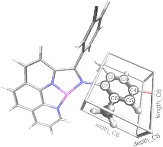Fig. 3 Illustration of features length_C6, width_C6, and depth_C6 for complex II (L₂ = Me, L₃ = Br, see Fig. 2a). C atoms are shown in gray, H in white, N in blue, Br in red, and Fe in purple.

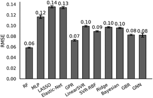
The Scikit-learn⁶⁰ Python library was used to set up and train regressors based on the aforementioned experimental dataset and features. Nine regression algorithms were tested, including random forest, least absolute shrinkage, and selection operator (LASSO), elastic-net, Gaussian process, ridge, Bayesian ridge, gradient-boosting, support vector regression with either a linear and radial basis function kernel, and a multi-layer perception (MLP). To avoid overfitting the machine learning model, we performed random sampling 100 times with the data set randomly split into 80% training and 20% testing sets each time. The RMSE of each model determined using random sampling averaged across 100 iterations is shown in Fig. 4. Additional data can be found in the ESI.† Results are also verified using 30-fold cross-validation averaged across ten iterations.

Fig. 4 Root mean squared error (RMSE) with 95% confidence intervals (bars) for machine learning regression algorithms to quantitatively predict K(C₁₂/C₁₀) values. All models except GNN used the 14 physical and chemical features. RF = random forest, MLP = multi-layer perceptron, LASSO = least absolute shrinkage and selection operator, GPR = Gaussian process regression with the rational quadratic kernel, GBR = gradient-boosting regression, SVR = support vector regression, GNN = graph neural network.

Additionally, a graph neural network (GNN) model was built using the Spektral Python library.⁶¹ GNNs use a graph representation of the molecule, where atoms are graph nodes and bonds are edges between nodes. Instead of the molecular features, one-hot encoded elements and bond orders were used as the properties for the nodes and edges. Through successive convolutions of adjacent nodes, information about the structure is shared to produce a set of weights. The weights are summed to give the predicted K-value. Our GNN model utilized six edge-conditioned convolution layers with 32 channels, as well as a global attention sum pool, which learns which node weights to sum during the training process. We did not include reaction conditions in the GNN model. The GNN model was subjected to the same cross validation methods as the other models.

The RMSE of all the regression algorithms ranged from 0.06 to 0.5 for the K-values. The best performing model was random forest (RMSE = 0.06). The random forest regressor is an ensemble (forest) of decision trees. Each tree is trained on a subset of the full training data set and, therefore, generates a slightly different prediction model. The final random forest model is the averaged results of all the decision trees. Random forest regressor is useful because it can generally handle outliers and unbalanced training data, and it is resistant to data overfitting. Other tested regressors showed similar performance, but they are slightly worse than the random forest (RMSE of ∼0.1). For Gaussian process regression, several kernels were tested. The rational quadratic kernel outperformed the Matérn (with ν = 3/2 and ν = 5/2) and radial basis function kernels, which tended to overfit during hyperparameter optimization. The performance of support vector regression improved significantly when changing from a linear (RMSE = 0.50) to a radial basis function kernel (RMSE = 0.12). The GNN model performed well with an RMSE of 0.07.

Results and discussion

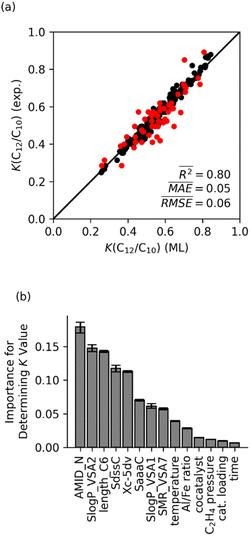
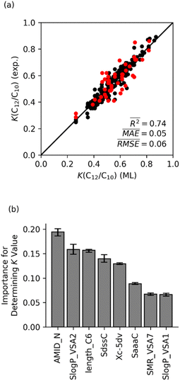
Fig. 5a shows the K(C₁₂/C₁₀) values calculated using the optimized random forest model are plotted versus the experimentally determined K-values. The optimized random forest K-value model agrees with experimental values very well (R² = 0.80, mean absolute error (MAE) = 0.05). Importantly, the accuracy of this machine learning model with an MAE for the K-value of 0.05 translates to this model having sub-kcal mol⁻¹ accuracy for selectivity within a statistical framework. This accuracy is significantly better than what is possible with either DFT or wavefunction type quantum-chemical calculations.^27,28

Fig. 5 (a) K(C₁₂/C₁₀) values predicted using random forest model with fourteen features, compared to experimental values. The training set is shown in black; testing set is shown in red. (b) Normalized feature importance determined from random forest model with 95% confidence intervals.

Indeed, propagation (migratory insertion) and termination (β-hydrogen transfer) transition-state energy calculations at the M06-L/def2-TZVP//M06-L/6-31G**[LANL2DZ for Fe]^62–69 level give K(C₁₂/C₁₀) values of 0 for all three complexes I (L₁ = Me, Et, iPr), predicting the absence of C-chain propagation during catalysis. In comparison, the experimentally measured K-values for complexes I (Fig. 2a; L₁ = Me, Et, iPr) range between 0.6 and 0.8 under varying reaction conditions. Initially, we hypothesized that DLPNO-CCSD(T) would be accurate enough, but single point DLPNO-CCSD(T) using DFT-optimized geometries with the RIJCOSX approximation⁷⁰ at both the def2-TZVP//def2-TZVP/C//def2/J level^71–75 also give K-values very close to 0, which is incompatible with experiment. Therefore, both DFT and DLPNO-CCSD(T) are not accurate enough to model this oligomerization selectivity.

Fig. 5b displays the feature importance for the random forest model. The AMID_N is statistically the most important feature for predicting Fe catalyst K-values, followed by SlogP_VSA2 and length_C6. The AMID_N is the average molecular ID of nitrogen atoms and characterizes molecular branching around the nitrogens.⁵⁴ It represents the number of paths around the molecule, weighted by bond orders and proximity to nitrogen atoms. SlogP_VSA2 pertains to the estimated surface area of relatively hydrophilic atoms.⁵⁶ As described above, the length_C6 parameter describes the size of ligand arm branching from the main ligand core surrounding the Fe metal center, which we have called a CSF feature. The relative importance of AMID_N and length_C6 suggests that the K-value of catalysts is heavily influenced by the steric impact of a ligand arms, as well as the general structure of the backbone. Although this interpretation is not overwhelmingly surprising, it demonstrates that chemical properties that control selectivity can be qualitatively identified through machine learning analysis.

Although the other molecular features are statistically less important, they are still very useful for the model and survived the feature selection process. These features either directly or indirectly describe the electronic nature of the ligand scaffold. The SdssC parameter, which sums the E-states of carbons with a double bond and two single bonds, is indicative of the family the ligand belongs to.⁵⁷ For ligands with two imines or an imine and a carbonyl, the value of SdssC is typically around 2–3. If there is just one imine (e.g., phenanthroline-imine ligands), the value is typically around 1–1.5. The closely related SaaaC parameter (i.e., sum of E-states on carbons with three aromatic bonds) can also be useful for differentiating ligands based on their backbone, since carbons with three aromatic bonds are only present in phenanthroline and α-diimine ligands in our training set. The SlogP-VSA1 parameter is the estimated surface area of very hydrophilic atoms.⁵⁶ This parameter provides an indirect measure of aromatic heteroatoms. Similarly, SMR-VSA7 estimates the surface area of relatively polarizable atoms.⁵⁶ For our training set, these are primarily aryl halides, atoms coordinated to the iron (which have a positive formal charge in our input structures), and aromatic carbons bonded to aliphatic carbons.

Even though the physical features (reaction conditions) have lower importance than molecular features, we note that the machine learning model can predict the changes in K-value with respect to different reaction conditions. To demonstrate this, we considered complex I (L₁ = methyl; Fig. 2a) under various reaction conditions. With changes in catalyst loading, co-catalyst loading (reported as molar Al/Fe ratio in literature), ethene pressure, reaction temperature, and time, the experimentally measured K-values for complex I (L₁ = Me) vary between 0.59 and 0.81 (Table 2). The K-values in Table 2 were removed from the training data set and then a new random forest model generated followed by prediction for these 11 structures. The random forest machine learning predicted K-values for complex I (L₁ = Me) are in good agreement with the experimental values. Fig. 6 plots the experimental K-values and the difference with the random forest predicted values.

Table 2 Experimental and machine learning predicted K(C₁₂/C₁₀) values of complex I (L₁ = Me) under various reaction conditions (taken from ref. 14). ML = random forest machine learning model

	Cat. loading^a (μmol)	Al/Fe molar ratio	Reaction length (min)	P (bar)	T (°C)	K (exp.)	K (ML)
a All pre-catalysts were activated with MMAO.
1	0.064	17656	60	48	120	0.59	0.62
2	0.06	18833	60	48	120	0.59	0.62
3	0.43	300	30	68	50	0.68	0.71
4	0.13	2000	30	203	90	0.70	0.70
5	0.13	2000	30	405	90	0.70	0.71
6	0.09	2000	30	608	90	0.70	0.70
7	0.24	2000	15	304	80	0.71	0.69
8	0.1	2000	30	203	60	0.73	0.73
9	0.1	2000	30	405	60	0.73	0.73
10	0.13	2000	120	203	35	0.74	0.74
11	5.7	700	180	1	25	0.81	0.76

---

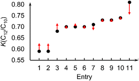Fig. 6 Experimental K(C₁₂/C₁₀) values of complex I (L1 = Me) (black dots) vary between 0.59 and 0.81 under different reaction conditions (Table 2).¹⁴ Red arrows indicate differences between the experimental K-values and the predicted K-values from a model utilizing the 6 physical and 8 molecular features.

We also determined the efficacy of the random forest model where either only physical or only molecular features were used. When only the six physical features were used, the random forest model was only able to predict K(C₁₂/C₁₀) values with moderate to poor accuracy (test set gave an averaged R² = 0.42 over 100 random samplings (see ESI†)). Despite the poor model performance, feature importance did reveal that the most important physical features for predicting K-value are the ethene pressure and then catalyst loading. However, both physical features show little importance in the random forest model when physical and molecular features are included.

In contrast to the random forest model with only physical features, a random forest model with only molecular features provides almost the same accuracy as the model with all 14 features. Fig. 7 shows that the random forest model predicted K(C₁₂/C₁₀) values with an averaged R² = 0.74, which is close to the R² value of 0.8 for the model shown in Fig. 5a. Analysis of the feature importance suggests that, like the physical and chemical model, the AMID_N, SlogP_VSA2, and length_C6 features are most important. Overall, the comparison of these models with only physical and only chemical features indicates that the selectivity for Fe ethene oligomerization catalysis is governed and dominated by the ligand impacting the steric and electronics of the Fe metal center and the transition states for propagation versus termination. Therefore, further examination of ligand steric and electronic effects was conducted using the optimized machine learning model with only chemical features.

Fig. 7 (a) Results from random forest model for K-value prediction using eight molecular features. The plot of predicted K(C₁₂/C₁₀) values versus experimental values. The training set is shown in black; the testing set is shown in red. (b) Normalized feature importance.

To demonstrate that this random forest model provides prediction of key steric effects, we used the model to examine the effect of methyl (–Me) versus ethyl (–Et) versus isopropyl (–iPr) groups in the aryl ortho position of ligand arms. This is important because it is extremely difficult, if not impossible, for DFT calculations to predict (quantitatively or qualitatively) this ligand effect. Within our experimental data set, fifteen sets of K-values, corresponding to eleven groups of catalysts, were considered. Each group of catalyst consists of three catalysts that have the same ligand backbone but have different substitutions on the phenyl-imine arm. Fig. 8 plots the experimental and machine learning predicted K-values for four representative catalysts, and the remainder are shown in ESI.† Importantly, this revealed that the machine learning model can capture relationships where the K-value increases with increasing group bulkiness, where the K-value has an inverse relationship group bulkiness, and where there is no specific pattern.

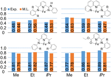Fig. 8 Machine learning predicted K(C₁₂/C₁₀) values (orange) compared with experimental values (blue). R = methyl (Me), ethyl (Et), or isopropyl (iPr) group.

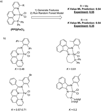
To begin to validate our machine learning model, we made a prediction for an Fe complex that had not previously been tested for olefin oligomerization selectivity. This new catalyst is shown in Fig. 9a and features a phosphaneyl–pyridinyl–quinoline (PPQ) type ligand structure.^76,77 The random forest machine learning predicted K-value for this (PPQ)Fe catalyst is 0.54. We subsequently synthesized the (PPQ)FeCl₂ and experimental measured the K(C₁₂/C₁₀) value under conditions similar to the harvested data used to create the machine learning model. The measured experimental value was 0.55. This validation demonstrates the potential quantitative utility of this machine learning model. However, like any machine learning model caution should be used when designing and predicting new catalysts, especially if they might be outside of the training data. This (PPQ)Fe catalyst fits within our training data because it has both a phosphine and pyridine type direct ligation to the Fe metal center. This experimental validation shows the utility of developing a specific machine learning to enable catalyst development. However, subtle chemical features are complex to accurately predict. Our machine learning model also predicts the same K-value for the (PPQ)Fe catalyst where the ortho-methyl group of the pyridyl ring is changed to a hydrogen. We also tested this catalyst, and the experimental K(C₁₂/C₁₀) value was 0.35, which is lower than the prediction and slightly outside the general error of the model. Therefore, again, while this machine learning model can be quantitative within the range of its training data, it is perhaps useful to qualitatively identify new potential catalysts with low, medium, or high K-values.

Fig. 9 (a) Use of the random forest machine learning model to predict the K-value for an Fe pyridylquinolinylphosphine catalyst. The measured K(C₁₂/C₁₀) value was within the machine learning model error. (b) Proximity analysis for the (PPQ)Fe catalyst. This shows the catalysts in the training data that provide strong proximity for the prediction.

In addition to generating K-value predictions for a new possible catalyst, this random forest model can also be used to report which catalysts from the training data provide the strongest descriptor information for prediction. Viewing structures that provide strong influence for the prediction can provide general confidence in the prediction as well as inspiration for new possible catalyst designs. Examining the most similar training data points for a given input provides inspiration for how the input could reasonably be modified to alter selectivity. Therefore, we have carried a so-called proximity analysis for the (PPQ)Fe catalyst (Fig. 9b). The proximity is the fraction of decision trees in the forest where that pair of inputs ends up on the same leaf node. A higher proximity generally indicates that those inputs are more similar. This gives a qualitative insight into the model prediction and a general evaluation of whether the prediction can be made with the current training data. In other words, if several training catalysts that have a high proximity value have similar partial ligand scaffolds to the catalyst under prediction, then there can be reasonable confidence that the prediction is within the capability of the model. In contrast, if the highest proximity training data have ligand substructures that are dramatically different than the predicted catalyst, then this should induce caution about the interpretation of the predicted value. Fig. 9b shows the four highest proximity catalysts for the (PPQ)Fe catalyst. Looking at these highest-proximity training points shows phenanthrolinyl-imine and type phosphanyl-acenaphthene-1,2-diimine (PNN) ligands provide a high degree of similar features to the PPQ ligand.

Conclusions

Machine learning models that enable the prediction of chemical properties hold the potential to significantly impact homogeneous catalyst design. However, machine learning models for homogeneous, molecular organometallic catalyst systems that use experimental selectivity data without incorporating quantum-mechanical calculations are rare.⁷⁸ In this work, we developed a sub-kcal mol⁻¹ accurate machine learning model for predicting linear α-olefin distributions K-values for Fe-catalyzed ethene oligomerization. This experiment-based machine learning model was developed using straightforward 2D molecular features and newly created ad hoc features. Importantly, this machine learning model captures the effects of a broad range of ligand architectures and replicates and predicts chemically nonintuitive trends in oligomerization α-olefin selectivity, especially for small ligand changes that cannot likely be capture even by extremely accurate quantum-chemistry methods. Our machine learning model was validated by the prediction and then experimental realization of a new (PPQ)Fe catalyst tested for olefin oligomerization. We also showed how a proximity analysis can be used for inspiration of additional designs. Due to the nature of random forest regressor, caution needs to be taken when the model is used for structures that are outside the chemical space of the experimental training data. Overall, this model provides the ability to predict oligomerization selectivity that will enable catalyst design and priority for testing. As with all machine learning models there is the need for continual experimental feedback and improvement of the model parameters. For example, in the future model parameter improvement might be possible with inclusion of 3D-type descriptors.

Data availability

The data supporting this article have been included as part of the ESI.† Machine learning code can be requested from the corresponding author at E-mail: dhe@byu.edu.

Author contributions

B. Y. collected the K-value database, developed new machine learning features, generated machine learning models, and wrote the original draft of the manuscript. A. J. S. generated and analyzed machine learning models, developed the proximity analysis, and drafted the manuscript. B. L. S. assisted in collecting the K-value database, analyzed machine learning data, analyzed experimental data, and edited the manuscript. J. A. L. synthesized and characterized organic ligands, ran experimental ethene oligomerization reactions, analyzed machine learning data, analyzed experimental data, and edited the manuscript. S. M. B. conceived of the project, reviewed the data, and edited the manuscript. M. S. W-G. conceived of the project, analyzed machine learning and experimental data, provided supervision, and edited the manuscript. D. H. E. conceived of the project, acquired funding, provided supervision, and edited the manuscript.

Conflicts of interest

A patent application has been filed for subject matter contained in this article.

Acknowledgements

We thank Brigham Young University and the Fulton Supercomputing Lab for computational resources. We thank Chevron Phillips Chemical for financial support.

Notes and references

1. G. R. Lappin, Alpha olefins applications handbook, Dekker, New York, 1989.
2. D. S. McGuinness, Chem. Rev., 2011, 111, 2321–2341.
3. E. F. Lutz, J. Chem. Educ., 1986, 63, 202.
4. Y. Minami, T. Takebe, M. Kanamaru and T. Okamoto, Polym. J., 2015, 47, 227–234.
5. A. Meiswinkel, A. Wöhl, W. Müller and H. Bölt, Presented in part at Catalysis, Innovative applications in petrochemistry and refining, Germany, 2011.
6. O. L. Sydora, Organometallics, 2019, 38, 997–1010.
7. A. Boudier, P.-A. R. Breuil, L. Magna, H. Olivier-Bourbigou and P. Braunstein, Chem. Commun., 2014, 50, 1398–1407.
8. G. J. P. Britovsek, M. Bruce, V. C. Gibson, B. S. Kimberley, P. J. Maddox, S. Mastroianni, S. J. McTavish, C. Redshaw, G. A. Solan, S. Strömberg, A. J. P. White and D. J. Williams, J. Am. Chem. Soc., 1999, 121, 8728–8740.
9. B. L. Small, M. Brookhart and A. M. A. Bennett, J. Am. Chem. Soc., 1998, 120, 4049–4050.
10. A. M. A. Bennett, US Pat., 5955555, 1999.
11. B. L. Small, Acc. Chem. Res., 2015, 48, 2599–2611.
12. Z. Wang, G. A. Solan, W. Zhang and W.-H. Sun, Coord. Chem. Rev., 2018, 363, 92–108.
13. Z. Wang, Q. Mahmood, W. Zhang and W.-H. Sun, in Advances in Organometallic Chemistry, ed. P. J. Pérez, Academic Press, 2023, vol. 79, pp. 41–86.
14. B. L. Small and M. Brookhart, J. Am. Chem. Soc., 1998, 120, 7143–7144.
15. J. Scott, S. Gambarotta, I. Korobkov and P. H. M. Budzelaar, J. Am. Chem. Soc., 2005, 127, 13019–13029.
16. C. Bianchini, G. Giambastiani, I. G. Rios, G. Mantovani, A. Meli and A. M. Segarra, Coord. Chem. Rev., 2006, 250, 1391–1418.
17. V. C. Gibson, C. Redshaw and G. A. Solan, Chem. Rev., 2007, 107, 1745–1776.
18. W. Zhang, W.-H. Sun and C. Redshaw, Dalton Trans., 2013, 42, 8988–8997.
19. P. J. Chirik, Angew. Chem., Int. Ed., 2017, 56, 5170–5181.
20. D.-H. Kwon, B. L. Small, O. L. Sydora, S. M. Bischof and D. H. Ess, J. Phys. Chem. C, 2019, 123, 3727–3739.
21. G. V. Schulz, Z. Phys. Chem. B, 1935, 30, 379–398.
22. P. J. Flory, J. Am. Chem. Soc., 1940, 62, 1561–1565.
23. C. T. Young, R. von Goetze, A. K. Tomov, F. Zaccaria and G. J. P. Britovsek, Top. Catal., 2020, 63, 294–318.
24. J. C. W. Lohrenz, T. K. Woo and T. Ziegler, J. Am. Chem. Soc., 1995, 117, 12793–12800.
25. I. E. Nifant'ev, L. Y. Ustynyuk and D. N. Laikov, Organometallics, 2001, 20, 5375–5393.
26. A. Fong, Y. Yuan, S. L. Ivry, S. L. Scott and B. Peters, ACS Catal., 2015, 5, 3360–3374.
27. Y. Guo, C. Riplinger, U. Becker, D. G. Liakos, Y. Minenkov, L. Cavallo and F. Neese, J. Chem. Phys., 2018, 148, 011101.
28. R. Raucoules, T. de Bruin, C. Adamo and P. Raybaud, Organometallics, 2011, 30, 3911–3914.
29. S. M. Maley, D.-H. Kwon, N. Rollins, J. C. Stanley, O. L. Sydora, S. M. Bischof and D. H. Ess, Chem. Sci., 2020, 11, 9665–9674.
30. K. T. Butler, D. W. Davies, H. Cartwright, O. Isayev and A. Walsh, Nature, 2018, 559, 547–555.
31. M. Meuwly, Chem. Rev., 2021, 121, 10218–10239.
32. K. Jorner, A. Tomberg, C. Bauer, C. Sköld and P.-O. Norrby, Nat. Rev. Chem, 2021, 5, 240–255.
33. J. P. Janet, C. Duan, A. Nandy, F. Liu and H. J. Kulik, Acc. Chem. Res., 2021, 54, 532–545.
34. S. M. Moosavi, K. M. Jablonka and B. Smit, J. Am. Chem. Soc., 2020, 142, 20273–20287.
35. T. Toyao, Z. Maeno, S. Takakusagi, T. Kamachi, I. Takigawa and K.-i. Shimizu, ACS Catal., 2020, 10, 2260–2297.
36. P. Friederich, G. dos Passos Gomes, R. De Bin, A. Aspuru-Guzik and D. Balcells, Chem. Sci., 2020, 11, 4584–4601.
37. Q.-Y. Liu, C. Shang and Z.-P. Liu, J. Am. Chem. Soc., 2021, 143, 11109–11120.
38. J. M. Crawford, C. Kingston, F. D. Toste and M. S. Sigman, Acc. Chem. Res., 2021, 54, 3136–3148.
39. S. Singh and R. B. Sunoj, Acc. Chem. Res., 2023, 56, 402–412.
40. B. L. Small, R. Rios, E. R. Fernandez, D. L. Gerlach, J. A. Halfen and M. J. Carney, Organometallics, 2010, 29, 6723–6731.
41. B. L. Small, R. Rios, E. R. Fernandez and M. J. Carney, Organometallics, 2007, 26, 1744–1749.
42. W.-H. Sun, X. Tang, T. Gao, B. Wu, W. Zhang and H. Ma, Organometallics, 2004, 23, 5037–5047.
43. W.-H. Sun, S. Jie, S. Zhang, W. Zhang, Y. Song, H. Ma, J. Chen, K. Wedeking and R. Fröhlich, Organometallics, 2006, 25, 666–677.
44. S. Jie, S. Zhang, W.-H. Sun, X. Kuang, T. Liu and J. Guo, J. Mol. Catal. A: Chem., 2007, 269, 85–96.
45. W.-H. Sun, P. Hao, S. Zhang, Q. Shi, W. Zuo, X. Tang and X. Lu, Organometallics, 2007, 26, 2720–2734.
46. Y. Chen, P. Hao, W. Zuo, K. Gao and W.-H. Sun, J. Organomet. Chem., 2008, 693, 1829–1840.
47. R. Gao, Y. Li, F. Wang, W.-H. Sun and M. Bochmann, Eur. J. Inorg. Chem., 2009, 2009, 4149–4156.
48. L. Xiao, R. Gao, M. Zhang, Y. Li, X. Cao and W.-H. Sun, Organometallics, 2009, 28, 2225–2233.
49. S. Song, R. Gao, M. Zhang, Y. Li, F. Wang and W.-H. Sun, Inorg. Chim. Acta, 2011, 376, 373–380.
50. M. Zhang, W. Zhang, T. Xiao, J.-F. Xiang, X. Hao and W.-H. Sun, J. Mol. Catal. A: Chem., 2010, 320, 92–96.
51. A. S. Ionkin, W. J. Marshall, D. J. Adelman, B. B. Fones, B. M. Fish and M. F. Schiffhauer, Organometallics, 2006, 25, 2978–2992.
52. A. S. Ionkin, W. J. Marshall, D. J. Adelman, B. Bobik Fones, B. M. Fish, M. F. Schiffhauer, R. E. Spence and T. Xie, Organometallics, 2008, 27, 1147–1156.
53. V. K. Appukuttan, Y. Liu, B. C. Son, C.-S. Ha, H. Suh and I. Kim, Organometallics, 2011, 30, 2285–2294.
54. M. Randic, J. Chem. Inf. Comput. Sci., 1984, 24, 164–175.
55. L. B. Kier and L. H. Hall, Molecular connectivity in structure-activity analysis, Research Studies, Letchworth, 1986.
56. P. Labute, J. Mol. Graphics Modell., 2000, 18, 464–477.
57. L. B. Kier and L. H. Hall, Pharm. Res., 1990, 7, 801–807.
58. H. Moriwaki, Y.-S. Tian, N. Kawashita and T. Takagi, J. Cheminf., 2018, 10, 4.
59. RDKit: Open-source Cheminformatics, http://www.rdkit.org.
60. F. Pedregosa, G. Varoquaux, A. Gramfort, V. Michel, B. Thirion, O. Grisel, M. Blondel, P. Prettenhofer, R. Weiss, V. Dubourg, J. Vanderplas, A. Passos, D. Cournapeau, M. Brucher, M. Perrot and E. Duchesnay, J. Mach. Learn. Res., 2011, 12, 2825–2830.
61. D. Grattarola and C. Alippi, IEEE Comput. Intell. Magaz., 2021, 16, 99–106.
62. Y. Zhao and D. G. Truhlar, J. Chem. Phys., 2006, 125, 194101.
63. R. Ditchfield, W. J. Hehre and J. A. Pople, J. Chem. Phys., 1971, 54, 724–728.
64. M. M. Francl, W. J. Pietro, W. J. Hehre, J. S. Binkley, M. S. Gordon, D. J. DeFrees and J. A. Pople, J. Chem. Phys., 1982, 77, 3654–3665.
65. M. S. Gordon, J. S. Binkley, J. A. Pople, W. J. Pietro and W. J. Hehre, J. Am. Chem. Soc., 1982, 104, 2797–2803.
66. P. C. Hariharan and J. A. Pople, Theor. Chim. Acta, 1973, 28, 213–222.
67. W. J. Hehre, R. Ditchfield and J. A. Pople, J. Chem. Phys., 1972, 56, 2257–2261.
68. V. A. Rassolov, M. A. Ratner, J. A. Pople, P. C. Redfern and L. A. Curtiss, J. Comput. Chem., 2001, 22, 976–984.
69. P. J. Hay and W. R. Wadt, J. Chem. Phys., 1985, 82, 299–310.
70. S. Kossmann and F. Neese, Chem. Phys. Lett., 2009, 481, 240–243.
71. F. Weigend and R. Ahlrichs, Phys. Chem. Chem. Phys., 2005, 7, 3297–3305.
72. F. Weigend, Phys. Chem. Chem. Phys., 2006, 8, 1057–1065.
73. A. Hellweg, C. Hättig, S. Höfener and W. Klopper, Theor. Chem. Acc., 2007, 117, 587–597.
74. J. Chmela and M. E. Harding, Mol. Phys., 2018, 116, 1523–1538.
75. D. Andrae, U. Häußermann, M. Dolg, H. Stoll and H. Preuß, Theor. Chim. Acta, 1990, 77, 123–141.
76. M. Kamitani, K. Yujiri and H. Yuge, Organometallics, 2020, 39, 3535–3539.
77. D. Basu, R. Gilbert-Wilson, D. L. Gray, T. B. Rauchfuss and A. K. Dash, Organometallics, 2018, 37, 2760–2768.
78. D. Ess, L. Gagliardi and S. Hammes-Schiffer, Chem. Rev., 2019, 119, 6507–6508.

---

Footnote

† Electronic supplementary information (ESI) available: Details on machine learning model including workflow, catalyst dataset, feature selection, and testing on steric effect (PDF). See DOI: https://doi.org/10.1039/d4sc03433c

---