DOI:
10.1039/D3SM00987D
(Paper)
Soft Matter, 2024,
20, 224-244
Pair-distribution function of active Brownian spheres in three spatial dimensions: simulation results and analytical representation†
Received
26th July 2023
, Accepted 3rd November 2023
First published on 6th November 2023
Abstract
The pair-distribution function, which provides information about correlations in a system of interacting particles, is one of the key objects of theoretical soft matter physics. In particular, it allows for microscopic insights into the phase behavior of active particles. While this function is by now well studied for two-dimensional active matter systems, the more complex and more realistic case of three-dimensional systems is not well understood by now. In this work, we analyze the full pair-distribution function of spherical active Brownian particles interacting via a Weeks–Chandler–Andersen potential in three spatial dimensions using Brownian dynamics simulations. Besides extracting the structure of the pair-distribution function from the simulations, we obtain an analytical representation for this function, parametrized by activity and concentration, which takes into account the symmetries of a homogeneous stationary state. Our results are useful as input to quantitative models of active Brownian particles and advance our understanding of the microstructure in dense active fluids.
I. Introduction
The study of active soft matter1,2 has been one of the most rapidly growing fields of physics in the past decade. Active particles convert energy into directed motion, as a consequence of which active matter systems are permanently driven out of equilibrium. This gives rise to a broad range of phenomena that are not possible in equilibrium (passive) systems. Examples of active matter include biological organisms like bacteria,3–5 birds,6 or fish,7 but also synthetic objects like self-propelled catalytic Janus particles.8
Rather than using a detailed description of living organisms, theoretical studies of the collective dynamics of active matter typically start from simple models. Among the most important one of these is the active Brownian particle (ABP), which exhibits a self-propulsion force with constant magnitude in a direction û that changes via rotational diffusion. ABPs exhibit interesting collective dynamics, with one of the most notable and widely studied phenomena being motility-induced phase separation (MIPS).9 Here, a system consisting of particles with purely repulsive interactions separates into a dilute gas phase and a dense cluster phase. Most studies of MIPS and the collective dynamics of ABPs focus on the two-dimensional case.10–26 The three-dimensional case has also attracted some attention,27–36 but is, due do its increased computational complexity, less well understood.
A central quantity of classical many-body physics is the pair-distribution function g, which determines the probability of finding two particles in a particular configuration. The importance of this function results, among other things, from the fact that it is used in microscopic derivations of field-theoretical models.37–41 For equilibrium systems, the pair-distribution function is well understood. It can be approximated analytically using liquid integral theory42–46 and has been thoroughly studied both in experiments47–51 and computer simulations.50,52 These results, however, do not generally carry over to the active case: since ABPs are far from thermodynamic equilibrium, their properties cannot be related to their bare interaction potentials alone. Instead, one needs to also take into account the effect of self-propulsion on the local properties. At the same time, the pair-distribution function has been found to be highly useful in understanding the microscopic origin of MIPS.11
The pair-distribution function of active particles has therefore attracted an increasing amount of interest in recent years.11,26,37,53–55 In particular, it has been investigated how this function depends on the activity and packing density of the particles, both in single-component systems11 and in mixtures of active and passive particles.37 Moreover, Härtel et al.54 have analyzed the three-body distribution and the full pair-distribution function of ABPs in two spatial dimensions. They also obtained an analytical expression for a reduced form of the pair-distribution function. Schwarzendahl et al.53 have studied the influence of hydrodynamic interactions on the pair-distribution function, and also investigated the (not fully orientation resolved) pair-distribution function of ABPs in three spatial dimensions. The orientational ordering and collective behaviour of pushers and pullers was investigated in ref. 55. Additionally, an approximate expression valid in the slow- and fast-swimming limits for the pair-distribution function of ABPs was derived by Dhont et al.56 The validity of this expression, however, is limited to packing densities below 0.1.56 Finally, a fully orientation-resolved pair-distribution function for a wide range of activities and packing densities in two spatial dimensions has been published recently by us,26 along with a software package that allows to reproduce this function.57 By comparing with the results from ref. 37 and 38 we furthermore observe that the availability of such a fully orientation-resolved distribution significantly improves theoretical predictions for the spinodal of MIPS.
However, until now there is no systematic analysis of the full orientation-resolved pair-distribution function of spherical ABPs for a wide range of activities and packing densities in three spatial dimensions. To close this gap, we study in this work the fully orientation-resolved pair-distribution function using Brownian dynamics simulations and examine its dependence on all relevant parameters for homogeneous stationary states. We also provide an analytical expression for the product of the interaction force and the pair-distribution function. This analytical expression has already been used in ref. 39 to find the spinodal and critical point of a system of ABPs.
This article is structured as follows. We explain our methodology and give an overview of the simulation details in Section II. In Section III, we present a high-resolution state diagram, the fully orientation-resolved pair-distribution function, and an analytical expression for the product of this function and the interaction force. We conclude in Section IV.
II. Methods
To analyze the pair-distribution function of spherical ABPs, we carried out Brownian dynamics simulations using a modified version of the software package LAMMPS.58
A. Model and simulation details
We study the dynamics of N spherical ABPs, described by overdamped Langevin equations.11,17,26,27 For the translational motion, they are given by| |  | (1) |
with the position ri of the i-th particle, the time t, the translational diffusion coefficient of passive spherical particles Dt = kBT/(3πση) resulting from the Stokes–Einstein relation, the Boltzmann constant kB, the absolute temperature T, the particle diameter σ, the dynamical viscosity η, the interaction potential U(r), the self-propulsion speed v0, the orientation of the i-th particle  , and the noise term ft,i(t). For U, we use the Weeks–Chandler–Andersen potential,59i.e., a truncated and shifted Lennard-Jones potential. This purely repulsive potential reads
| |  | (2) |
with the interaction strength ε. The noise term ft,i(t) is modeled using Gaussian white noise with the properties 〈ft,i(t) ⊗ ft,j(t′)〉 = 2Dtδi,jδ(t − t′)![[1 with combining low line]](https://www.rsc.org/images/entities/char_0031_0332.gif) , where ⊗ is the dyadic product and
, where ⊗ is the dyadic product and ![[1 with combining low line]](https://www.rsc.org/images/entities/char_0031_0332.gif) the identity matrix. To quantify the ratio between active and thermal forces, we use (as is common) the Péclet number Pe = v0σ/Dt.
the identity matrix. To quantify the ratio between active and thermal forces, we use (as is common) the Péclet number Pe = v0σ/Dt.
The rotational motion of the particle is given by
| |  | (3) |
with
fr,i(
t) being a noise term that is characterized as Gaussian white noise with the properties 〈
fr,i(
t) ⊗
fr,j(
t′)〉 = 2
Drδi,jδ(
t −
t′)
![[1 with combining low line]](https://www.rsc.org/images/entities/char_0031_0332.gif)
. Here,
Dr is the rotational diffusion coefficient that for spherical particles in a viscous fluid is given by the Stokes–Einstein–Debye relation
Dr =
kBT/(π
σ3η) = 3
Dt/
σ2. The swimming speed of a particle is
v0 = 24
σ/
τLJ = 24
Dtε/(
σkBT), such that the repulsive force of the potential at
r =
σ is equal to the force corresponding to self-propulsion. We vary the Péclet number by changing the temperature:
26,27 as the temperature diverges for small Péclet numbers, we vary Pe between 50 and 500. We use the Lennard-Jones units
τLJ =
σ2/(
εβDt),
σ, and
ε as units of time, length, and energy, respectively.
Besides the Péclet number, we vary the average packing density Φ0 = πσ3N/(6V) (where V is the volume of the domain) by changing the particle number N. The domain is a cubic box with periodic boundary conditions and side length 30σ. Varying Φ0 from 0.05 to 0.7 corresponds to N ∈ [2578, 36![[thin space (1/6-em)]](https://www.rsc.org/images/entities/char_2009.gif) 096]. The particles were initially placed on a hexagonal grid to prevent strong overlapping. After an initial simulation time of 150τLJ at a low Péclet number (Pe = 50), the positions of the particles are relaxed to the steady state distribution. Then, the pair-distribution function was analyzed by sampling the system configuration at regular time intervals and binning the relative configuration for all particle pairs with a distance less than 10σ. Aiming for an average of 500 entries in the bins for the distance r = σ, we chose the simulation time according to the number of particles in the simulation. Thus, the simulation time scaled quadratically with the inverse of the number of particles and varied between 2.4 × 10⁴τLJ and 4.7 × 10⁶τLJ depending on Φ0. The time step size was 5 × 10⁻⁵τLJ and the time between samples was chosen such that a noninteracting self-propelled particle would be displaced by twice its diameter.
096]. The particles were initially placed on a hexagonal grid to prevent strong overlapping. After an initial simulation time of 150τLJ at a low Péclet number (Pe = 50), the positions of the particles are relaxed to the steady state distribution. Then, the pair-distribution function was analyzed by sampling the system configuration at regular time intervals and binning the relative configuration for all particle pairs with a distance less than 10σ. Aiming for an average of 500 entries in the bins for the distance r = σ, we chose the simulation time according to the number of particles in the simulation. Thus, the simulation time scaled quadratically with the inverse of the number of particles and varied between 2.4 × 10⁴τLJ and 4.7 × 10⁶τLJ depending on Φ0. The time step size was 5 × 10⁻⁵τLJ and the time between samples was chosen such that a noninteracting self-propelled particle would be displaced by twice its diameter.
To distinguish between a system undergoing phase separation and a homogeneous system, we used the characteristic length Lc. This length quantifies density inhomogeneities and can therefore be used as a measure for phase separation.27 It is defined as27
| |  | (4) |
Here,
S(
k,
t) is the structure factor
60| |  | (5) |
〈·〉 the average over the stationary state,
L the domain size,
kcut a cutoff wavelength, and
k = ‖
k‖ the norm of the wave vector
k. We here chose
kcut = π, which approximately coincides with the first minimum of
S(
k,
t). A high characteristic length corresponds to a high degree of spatial order,
i.e., to phase separation, which was confirmed by visual inspection. The characteristic length was sampled with a time resolution of 0.42
τLJ for a total simulation time between 5 × 10
3τLJ and 1.5 × 10
2τLJ scaling inversely with the packing density. At the beginning of each simulation, an additional simulation time of 100
τLJ was added to allow for relaxation. For each parameter combination in the state diagram (see below), six simulations were performed. The characteristic length was first averaged over the last 21
τLJ,
i.e., 50 samples, of each simulation, and then averaged over the different simulations. Due to the metastability of the homogeneous state in the binodal region, it is sensible to perform multiple simulations starting from different initial conditions for each parameter combination. Typically, the rapid change in characteristic length marking the spontaneous transition between homogeneous and clustered state happens on the timescale of a few
τLJ within the first 20
τLJ of the simulation. As the characteristic length remains virtually constant after this, the comparatively short simulation times were sufficient. Performing multiple simulations for each parameter combination, we confirmed the stability of the homogeneous distribution for parameter combinations close to the state boundary that will be used to examine the pair-distribution function.
B. Parametrization of the pair-distribution function
Let P({ri}, {ûi}, t) be the probability that the system is, at time t, in the microscopic configuration specified by the coordinates ri and ûi. In this case, we can define the n-particle density as| |  | (6) |
where  is the unit sphere in three spatial dimensions. This allows to define the pair-distribution function as46
| |  | (7) |
with ϱ = ϱ(1). The two-body density ϱ(2)(r1, r2, û1, û2, t) gives the probability of finding one particle with orientation û1 at position r1 and another particle with orientation û2 at position r2 at time t, and the one-body density ϱ(r1, û1, t) gives the probability of finding one particle with orientation û1 at position r1 at time t. If we use now the definition61| |  | (8) |
of the conditional probability of an event A given an event B, we can see that the product ϱ(r2, û2, t)g(r1, r2, û1, û2, t) is simply the conditional probability of finding, at time t, a particle with orientation û2 at position r2 given that another particle with orientation û1 is at position r1.62 Since we focus on spatially homogeneous one-particle distributions in this work, we will, with a slight abuse of terminology, sometimes simply refer to g as “probability”. Note, however, that strictly speaking g is not a probability, but proportional to a conditional probability (this conditional probability is determined by g once ϱ is fixed).
The importance of the pair-distribution function in active systems, in particular also of its orientation dependence, lies, among other things, in its role for motility-induced phase separation (MIPS). This phenomenon is essentially caused by an anisotropy of g.11 In equilibrium, g would have no angular dependence for spherical particles. However, in the case of self-propelled spheres, particles are more likely to be found in front of the particle than behind it, which reduces their effective swimming speed11 in a way that depends on the particle density. This density-dependent swimming speed is what is responsible for MIPS.10 Therefore, an understanding of the orientation dependence of g is crucial for understanding the nonequilibrium correlations in the system and thereby for understanding MIPS. Such an understanding will be provided for the three-dimensional case in the following.
A nondimensionalization of the Langevin eqn (1) and (3) shows that the dynamics can be expressed via two dimensionless parameters, namely the Péclet number Pe, which gives the ratio of active and thermal forces, and the product εβ, which gives the ratio of interaction and thermal forces. In general, the pair-distribution function can thus have a parametric dependence on Pe, εβ, and the packing density Φ0. In this work, we (as discussed in Section IIA) always choose v0 = 24σ/τLJ, implying that we fix Pe/(εβ) = 24 and thus only explicitly consider the dependence on Pe. An even more general approach would be to also vary εβ at fixed Pe. (It is known that, for a Weeks–Chandler–Andersen potential, g has a weak dependence on the temperature also in the passive case,63 an effect that is obviously not captured by only investigating the activity parameter Pe.) Moreover, if we would not assume Dt and Dr to be connected by the equilibrium relation Dr = Dt/σ2 (an assumption that is often not made in recent work), we could vary Dr separately at fixed σ, giving one further parameter that g could depend on. With these restrictions, the full pair-distribution function g(Pe, Φ0; r1, r2, û1, û2, t) depends on the Péclet number Pe, the packing density Φ0, the position and orientation of both particles, and the time t.
To simplify the pair-distribution function, we assume a stationary and homogeneous system. This allows us to drop the time dependence of g and to reduce the dependency on the absolute positions of the two particles to one on their relative positions. In total, the pair-distribution function g then depends only on the Péclet number Pe, the packing density Φ0, the particles' relative position r2 − r1 = r = rûd and the orientation ûi of each particle:
| | | g(Pe, Φ0; r, ûd, û1, û2). | (9) |
For the sake of brevity, we omit the explicit dependency on Pe and
Φ0 in our notation for the rest of this section. We can also exploit the isotropy of the system to eliminate some orientational dependencies of
g. For this, we first define a coordinate system with its origin at the center of the first particle and the
z-axis aligned with its orientation. Furthermore, we fix the
x-axis such that both particles lie in the
x–
z plane with the second particle at a positive
x coordinate as shown in
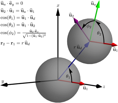
Fig. 1. Thus the orientation of the first particle is fixed. The relative position vector
rûd is now fixed to the
x–
z-plane and can be defined by the interparticle distance
r and the angle
θ1 between
û1 and
ûd. The orientation of the second particle can be expressed
via two angles. We choose the polar angle
θ2 and the azimuthal angle
ϕ2 as shown in
Fig. 1. Thus, the pair-distribution function only depends on four variables,
i.e.,
g =
g(
r,
θ1,
θ2,
ϕ2). The distance
r can furthermore be calculated
viaand the angles
θ1 and
θ2 are given by
The unit vector in
x-direction
êx can be obtained
via the cross product of the unit vector in
y-direction
êy and
û1, while
êy is obtained by calculating
û1 ×
ûd and normalizing the resulting vector
via division by sin(
θ1):
| |  | (13) |
The scalar product of
êx and the normalized projection of
û2 onto the
x–
y-plane is used to calculate
ϕ2. The projection is achieved by discarding the
z-component and normalizing the resulting vector. Normalizing the projection corresponds to a division by

. As
êx is orthogonal to the
z-axis, the
z-component of
û2 does not need to be discarded and the normalization is sufficient. The angle
ϕ2 is equal to the angle between the projections of
û2 into the
x–
y-plane and the
x-axis:
| |  | (14) |
There are coordinate singularities at sin(
θ1) = 0 and at sin(
θ2) = 0,
i.e., for
θ1 ∈ {0,π} and
θ2 ∈ {0,π}. The singularity for
θ2 ∈ {0,π} (
i.e., at the poles) is typical for spherical coordinates. In contrast, the singularity for
θ1 ∈ {0,π} (
i.e., when
û1‖
ûd) occurs due to the choice of
x- and
y-axis, which makes
ϕ2 ambiguous in this case.
 |
| | Fig. 1 Parametrization of the fully orientation-resolved pair-distribution function. The center of the coordinate system coincides with the center of the first particle and the z-axis is parallel to the orientation û1 of the first particle. The angle θ1 is the angle between the orientation of the first particle and the vector ud = rûd that connects the two particles, r the distance between the particles, and the angles θ2 and ϕ2 correspond to the polar and azimuthal angle, respectively, of the second particle's orientation û2 relative to that of the first particle. The vector ûa is a supportive vector in the x–z-plane that has the same polar angle as û2. | |
The pair-distribution function possesses several angular symmetries, in particular
| | | g(r, θ1, θ2, ϕ2) = g(r, θ1, θ2, −ϕ2), | (15a) |
| | | g(r, θ1, θ2, ϕ2) = g(r, −θ1, θ2, π − ϕ2), | (15b) |
| | | g(r, θ1, θ2, ϕ2) = g(r, θ1, −θ2, π − ϕ2). | (15c) |
By definition, the angles
θ1 and
θ2 are limited to the interval [0,π]. With the symmetries
(15a)–(15c), however, we can extend their definition to all angles in the interval [0,2π], making the pair-distribution function 2π-periodic in all angular parameters. This extension allows us to obtain a Fourier transformation of the pair-distribution function later. For simplicity, we always refer to the periodically extended version of the pair-distribution function in the following.
We measured the angles with a resolution of 2° resulting in Nb = 180 bins for each angular parameter for the interval [0,2π]. The bin size of the distance parameter r was chosen in a non-uniform way. Values smaller than 1.2σ were sampled with a bin size of 0.005σ, while for values smaller than 3σ a bin size of 0.02σ and for 3σ < r < 10σ a bin size of 0.05σ was chosen. We did not sample for any correlations beyond a distance of r = 10σ.
C. Orientation-averaged distribution function and relation to experiments
The pair-distribution function is often obtained in diffraction experiments.64 How this can be achieved is discussed in detail in ref. 46. In a nutshell, one obtains from experiment the structure factor S and calculates from this the experimentally obtained pair-distribution function gexp using the relation46| |  | (16) |
with the spatial number density ρ. The derivation of eqn (16) assumes the pair-distribution function to be defined as| |  | (17) |
which can be rewritten in the form| | | ρ(2)(r1,r2,t) = gexp(r1,r2,t)ρ(r1,t)ρ(r2,t) | (18) |
with the two-body density ρ(2) that gives the probability of finding a particle at position r1 and another one at position r2. This is a consequence of the fact that ref. 46 considers passive fluids, where (if the particles are spherical) a particle orientation cannot be meaningfully defined, implying that all densities and distribution functions depend only on the particle positions.
In an active system, the full pair-distribution function g depends also on the particle orientations. We can nevertheless still use the definition (17) of the experimental pair-distribution function g if we define ρ and ρ(2) as
| |  | (19) |
| |  | (20) |
If one does a neutron scattering experiment on a fluid consisting of APBs and calculates the pair-distribution function from the results using
eqn (16), what one obtains is the function
gexp, which depends only on the particle positions. It is therefore worth discussing how this function relates to the function
g discussed here, which is required for understanding the orientational dynamics of the ABPs and for the derivation of field theories.
From eqn (7), we find
| |  | (21) |
which together with
eqn (20) implies
| |  | (22) |
If we assume that the dependence of
ϱ on the particle orientation can be neglected, which by
eqn (19) implies that
ρ(
r1,
t) = 4π
ϱ(
r1,
t),
eqn (22) can be rewritten as
| |  | (23) |
with the orientation-averaged pair-distribution function
| |  | (24) |
Eqn (18) and (23) imply that in the case of a weak orientation dependence of
ϱ, the experimentally measured pair-distribution function
gexp is equal to the orientation-averaged pair-distribution function
gav. In general, this is not the case. Fortunately, in the homogeneous state, which is considered in our analysis of the ABP pair-distribution function, the orientation-dependence of
ϱ is indeed weak, such that our results can be directly compared to experiments.
III. Results and discussion
The parametrization used for g(Pe, Φ0; r, θ1, θ2, ϕ2) requires the system to be in a homogeneous state. Thus, we investigated the characteristic length Lc for different values of Pe and Φ0 to determine the regions in parameter space where the homogeneous state is stable. The results are shown in Fig. 2. It can be seen that the parameter space is split into two cohesive regions where either the homogeneous distribution is stable or phase separation occurs. More precisely, the system remains homogeneous over time if either Φ0 < 0.35 or Pe < 100. Outside this region, the system can exhibit phase separation. This becomes more favorable for high Péclet numbers and is suppressed only for very high densities. Here, we have a notable difference to the two-dimensional case discussed in ref. 26. In the two-dimensional case, the packing density of ABPs in a cluster can exceed the packing density of a perfect hexagonal structure of circles – the highest possible packing density for impenetrable spheres – due to overlapping.27 Therefore, phase separation occurs. In the three-dimensional case, however, the packing density of particles in a cluster is lower than the perfect packing density of an fcc grid, even though slight overlapping is possible.27 Consequently, the packing density of a “cluster” is not higher than the packing density of its environment, and therefore there is no phase separation. This argument, of course, hangs on the way we have defined the order parameter and therefore on our characterization of what “phase separation” is. If we, as done here, use the characteristic length, then the system will not be understood as being in a phase separated state if particles are everywhere (which is the case in three dimensions at high densities) since it then is homogeneous. In two dimensions, on the other hand, the fact that the particle density is extremely high in the cluster region has the consequence that there are fewer particles in another region, such that there is a finite characteristic length.
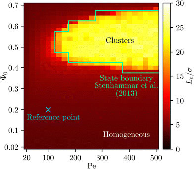 |
| | Fig. 2 State diagram for ABPs in three spatial dimensions. The characteristic length Lc described by eqn (4) quantifies density inhomogeneities which are characteristic for a clustered state thus allowing to identify regions of qualitatively different collective behavior. For comparison, the state boundary found by Stenhammar et al.27 is shown as well. The blue cross indicates the reference point at Pe = 100 and Φ0 = 0.2 used in the following figures. A file containing the raw data for Lc shown here is provided as ESI.†![[thin space (1/6-em)]](https://www.rsc.org/images/entities/char_2009.gif) 65 65 | |
Note that the state boundary found here is likely to be rather close to the spinodal. The reason is that, in the parameter region that is inside the binodal and outside the spinodal, both homogeneous states and clusters are (meta-)stable. In our simulations, we start with a homogeneous configuration and therefore end up in a homogeneous configuration in this region, but a simulation with an initial cluster could, in this region, have led to a final state with cluster formation.
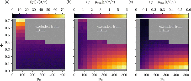
Our results confirm the state diagram by Stenhammar et al.27 and allow us to determine the regions where the symmetry assumptions introduced in Section IIB are valid (namely the regions where the particle distribution is homogeneous). The parameter combinations for which samples were taken to approximate g analytically are shown in Fig. 3.
 |
| | Fig. 3 Areas excluded from fitting and results for the product function p (see Section IIIB). (a) Mean absolute value (MAV) 〈|p|〉/(σ/ε) of the simulation data, (b) mean absolute error (MAE) 〈|p − papp|〉/(σ/ε) between the simulation data and the analytical approximation, and (c) the relative error MAE/MAV. The relative error is especially small for high packing densities and low Péclet number, and then grows with increasing Péclet number and shrinking packing density. The grey areas are excluded from fitting, as phase separation was observed for these parameter combinations. | |
To check whether this state diagram contains finite size effects, we also investigated the state diagram of a system with twice the size in each dimension resulting in an eight times higher particle number. The resulting state boundary widens up slightly, indicating phase separation for marginally smaller and higher densities. The critical Péclet number and density are not affected by the size of the system.
A. Pair-distribution function
The pair-distribution function is shown for selected configurations in Fig. 4, 6, and 7 for Pe = 100 and Φ0 = 0.2. These values have been chosen since they are deep in the homogeneous state (see Fig. 2).
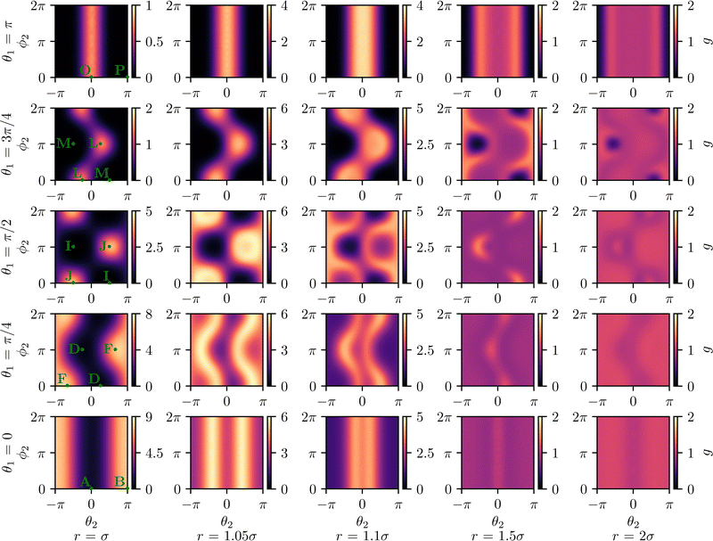 |
| | Fig. 4 Pair-distribution function g(Pe, Φ0; r, θ1, θ2, ϕ2) for distances r ∈ {σ, 1.05σ, 1.1σ, 1.5σ, 2σ} and angles θ1 ∈ {0, π/4, π/2, 3π/4, π} with fixed parameter values Pe = 100 and Φ0 = 0.2. This figure indicates the probability of finding a second particle with a prescribed position at different polar and azimuthal angles relative to a particle. The configurations marked in green, which are shown in Fig. 5, represent extrema of this probability. | |
Finding that the pair-distribution function can, with high accuracy, be represented by 15 Fourier modes, we use a low pass filter to cut off high frequencies in the angular dependence at the frequency ωcut = 15·2π = 30π to minimize statistical errors. For large distances, g goes to 1 since the probability of finding a particle at a position r2 is not influenced by the fact that another particle is at position r1 if r1 and r2 are very far apart.
We present g for values of r ∈ {σ, 1.05σ, 1.1σ, 1.5σ, 2σ}, which allows us to capture the most significant features of the pair-distribution function. Fig. 4 shows the pair-distribution function for a selection of fixed distances r and angles θ1. For each pair (r,θ1), we plot g as a function of θ2 and ϕ2. Therefore, each plot in Fig. 4 corresponds to a fixed position of the second particle relative to the first particle and indicates the probability for every possible orientation of the second particle. Similarly, Fig. 6 presents g for fixed distances r and polar angles θ2. For each pair (r,θ2), g is plotted as a function of θ1 and ϕ2. Finally, Fig. 7 displays g for fixed distances r and azimuthal angles of the second particle ϕ2. For each pair (r,ϕ2), g is plotted as a function of θ1 and θ2. Certain configurations, which are highlighted in Fig. 4, 6 and 7, are visualized in Fig. 5.
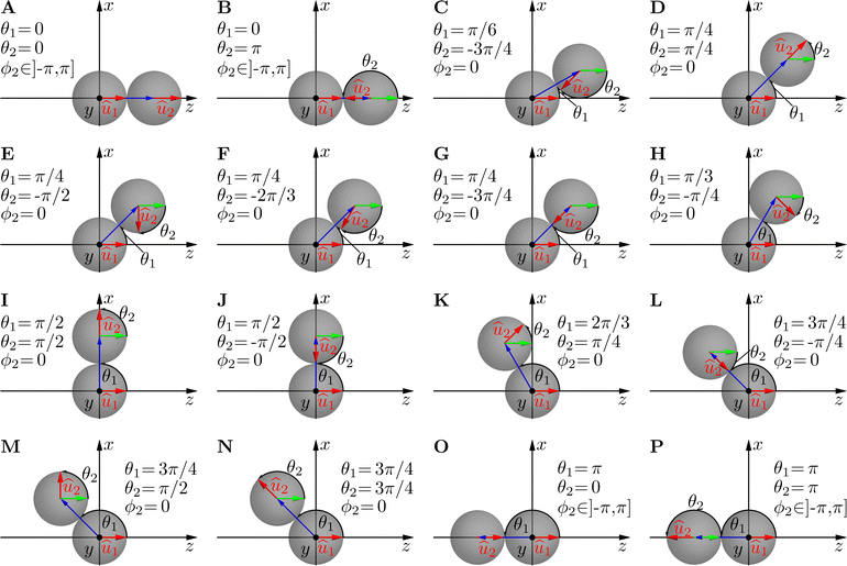 |
| | Fig. 5 Exemplary configurations of the particles that correspond to local extrema of the pair-distribution function g at r = σ. These configurations are marked as green dots in Fig. 4, 6 and 7. | |
In general, maxima of g are found for configurations that are very stable or easy to reach. Similarly, minima of g are found for configurations that are very unstable or impossible to reach. An example of a maximum of g is the configuration B in Fig. 5 with θ1 = 0, θ2 = π, and ϕ2 ∈ [−π, π]. In this case, the two particles are oriented towards each other and thus obstruct each other's motion until diffusion breaks up this configuration. Therefore, this configuration is very stable. In contrast, the configuration P in Fig. 5 with θ1 = π, θ2 = π, and ϕ2∈ [−π, π], i.e., two particles facing away from each other, coincides with a minimum of g. The reason is that (if we ignore thermal fluctuations) the only way to reach this configuration is that the particles move through each other (which is not possible for the interaction potential chosen here). As the repulsive interaction potential extends slightly further than r = σ, the pair-distribution function yields local maxima for r = σ where the particles' propulsion force pushes the particles towards each other (e.g., configurations B, F, J, L, and O of Fig. 5 marked in Fig. 4) and minima, where the interparticle force is minimized (e.g., configurations A, D, I, M, and P of Fig. 5 marked in Fig. 4). This line of reasoning also applies to the configurations in Fig. 6 and 7.
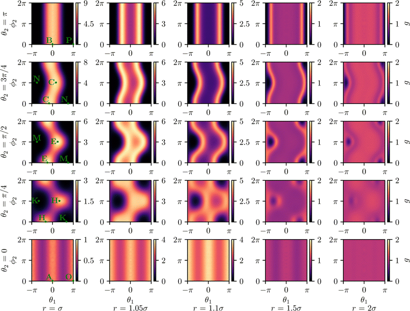 |
| | Fig. 6 Pair-distribution function g(Pe, Φ0; r, θ1, θ2, ϕ2) for distances r ∈ {σ, 1.05σ, 1.1σ, 1.5σ, 2σ} and angles θ2 ∈ {0, π/4, π/2, 3π/4, π} with fixed parameter values Pe = 100 and Φ0 = 0.2. This figure indicates the probability of finding a second particle with a prescribed polar angle at different positions and azimuthal angles relative to a particle. The configurations marked in green, which are shown in Fig. 5, represent extrema of this probability. | |
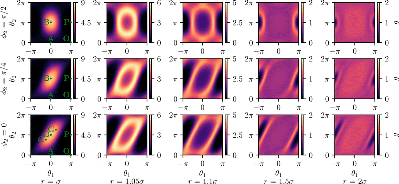 |
| | Fig. 7 Pair-distribution function g(Pe, Φ0; r, θ1, θ2, ϕ2) for distances r ∈ {σ, 1.05σ, 1.1σ, 1.5σ, 2σ} and angles ϕ2 ∈ {0, π/4, π/2} with fixed parameter values Pe = 100 and Φ0 = 0.2. This figure indicates the probability of finding a second particle with a prescribed azimuthal angle at different positions and polar angles relative to a particle. The configurations marked in green, which are shown in Fig. 5, represent extrema of this probability. | |
For slightly larger distances such as r = 1.05σ and r = 1.1σ, we find that the maxima broaden and create small local minima in their center. If the particles do not perfectly face each other, the interparticle force and propulsive force balance each other at a slightly larger separation.
The distribution function shows a change of structure for distances around r = 1.5σ. As particles cannot pass through each other, but, due to the overdamped motion, also do not bounce back after a collision,66 colliding particles often slide past each other. Therefore, configurations which result from particles moving past each other at a very small distance are more likely than configurations which result from particles moving past each other at a larger distance, as the latter happens only at random and not systematically due to interactions.
In similar cases, a configuration resulting from particles sliding past each other (high probability) and a configuration that can essentially only be reached by particles passing through each other (low probability) are only separated by small offsets in the respective angles. Therefore, some configurations that can practically only emerge from particles passing through each other, such as the configurations M, N, and K, are surrounded by local maxima.
If the azimuthal angle ϕ2 is zero, both orientation vectors û1 and û2 and the connecting vector ud lie in the same plane, such that the configuration is quasi-two-dimensional. The pair-distribution function for this scenario is plotted in the bottom row of Fig. 7. Note that the pair-distribution function is very similar to the pair-distribution function for a two-dimensional system obtained in ref. 26, which confirms our results.
We find that varying the Péclet number does not change the general structure of the pair-distribution function. Increasing the Péclet number and thus reducing the temperature merely sharpens the features of g in the form of taller and more narrow peaks of probability. This makes sense considering that probability peaks in g representing stable particle configurations are widened by rotational and translational diffusion, which diminish with decreasing temperatures.
In the case of low densities, in most cases only two particles interact with each other at a time. If the density increases, the probability of interactions between three or more particles increases. If several particles are involved in a collision, the resulting interactions that determine the pair-distribution function become more complex and the structure of g therefore becomes less sharp. Consequently, the effect of increasing the density is to broaden the maxima and minima of g.
In Fig. 8, we show in addition the orientation-averaged pair-distribution function gav of ABPs, defined in eqn (24), for different values of Pe and Φ0. Since the orientation-dependence of ϱ is weak in the homogeneous state, this corresponds to what would be measured in scattering experiments performed on the ABP system. The general shape of gav(r) is similar to that known from passive fluids.46 Comparing the curves for Φ0 = 0.2 and Φ0 = 0.4 (both with Pe = 100) shows that increasing Φ0 leads to more pronounced peaks, i.e., to higher spatial order. This is reasonable given that strong packing can lead to crystallization. Increasing Pe does, on the other hand, not have a very strong effect on the shape of gav (as can be seen from comparing the curves with Pe = 100 and Pe = 200 at Φ0 = 0.2). It leads to a larger first peak, implying that particles are more likely to be found close to another particle in the case of high activity.
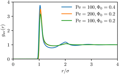 |
| | Fig. 8 Orientation-averaged pair-distribution function gav(r) of ABPs for several values of Pe and Φ0. | |
B. Analytical approximation of the function −gU′
One of the main reasons why the pair-distribution function is important is that it is required for deriving field theories.11,37,40,67,68 To see why, note that the dynamics of ϱ for a system of ABPs in three dimensions is given by39| |  | (25) |
with the interaction term| |  | (26) |
Here U′(r) = −dU2(r)/dr is the interparticle force and  the rotational operator. If (an approximation for) g is not known, we cannot (not even approximately) evaluate the integral in eqn (26). Therefore, field-theoretical models such as eqn (25) require an approximate analytical expression for g as an input. Once such an expression has been provided, the then closed dynamic equation for ϱ can be approximated further. This is done in the interaction-expansion method,37–39,69,70 which is reviewed in ref. 40.
Taking a closer look at eqn (26), we can see that what we actually require is not g, but the product of g and U′. Therefore, we now develop an analytical representation71 for the product function
| | | p(Pe, Φ0; r, θ1, θ2, ϕ2) = −U′(r)g(Pe, Φ0; r, θ1, θ2, ϕ2), | (27) |
which can be interpreted as a “pair-interaction-force distribution”. In contrast to the pair-distribution function
g, the product function
p is nonzero only for 0.9
σ <
r < 2
1/6σ.
72 The reason for this is that
g vanishes for
r less than approximately
σ due to the strong repulsion and
U′ vanishes for
r > 2
1/6σ due to the cutoff in the interaction force. Thus,
p only needs to be fitted in a narrow interval of
r.
The function p depends on the three angles θ1, θ2, and ϕ2, the distance r, the Péclet number Pe, and the packing density Φ0. First, we perform the real Fourier expansion
| |  | (28) |
with
and
| | 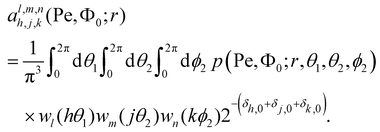 | (31) |
In our case,
p is not continuous but discrete since we use histograms for the data evaluation. This has to be accounted for in the definition of the coefficients
via| | 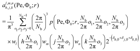 | (32) |
with the number of bins
Nb. Using the symmetries of
g shown in
eqn (15), one can show that many coefficients vanish. We find that the Fourier modes up to second order are sufficient for reproducing the structure of the product function reasonably well (similar to ref.
26).
73Fig. 3 shows that this truncation results only in a small error. This results in the approximation
| | 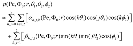 | (33) |
with
αh,j,k =
a1,1,1h,j,k and
βh,j,k =
a2,2,1h,j,k. We thus have 22 coefficients in total, each depending on
r, Pe, and
Φ0. In Appendix A, we discuss how the dependence of the coefficients on
r is fitted. The described fitting procedure allows us to describe four of the six parameter dependencies of
p(Pe,
Φ0;
r,
θ1,
θ2,
ϕ2) analytically and only the dependencies of the fit parameters on Pe and
Φ0 remain unknown. In order to get a purely analytical expression for
p, this dependence also needs to be interpolated for the region of parameter space shown in
Fig. 3. For this we use the empirically motivated fit function
| |  | (34) |
with the fit parameters
qm,n. The results of these fits are given in Appendix B.
To estimate the quality of our approximations, we calculate the deviation of our analytical approximations papp from the numerical result for p measured directly from simulation. We quantify the difference via the mean absolute error (MAE)
| |  | (35) |
In this case,
rmax equals

as the interaction potential is zero for higher values of
r and
rmin equals 0.8
σ as no two particles with a smaller distance were found in the simulations. For the relative error, we calculate the ratio between the MAE and the mean absolute value (MAV) of
p| |  | (36) |
In
Fig. 3, we show the MAE, the MAV, and the relative error MAE/MAV. The relative error varies between 2 and 55 percent with high errors occurring only for very small packing densities and very high Péclet numbers. We find that the errors are predominantly introduced by the frequency cutoff approximation and not by the two fitting steps. The reason for the high errors observed for low densities and high Péclet number are the high frequency modes of
g in this regime that result from the steeper slope of
g (see Section IIIA).
IV. Conclusions
In this work, we have obtained the state diagram and the full pair-distribution function of ABPs in three spatial dimensions using Brownian dynamics simulations. Our results confirm and improve state diagrams obtained in previous works.27–29 Note that the state boundary found in this work corresponds to the spinodal rather than to the binodal. Furthermore, the fully orientation-resolved pair-distribution function for homogeneous particle distributions has been extracted from the simulations for a wide range of Péclet numbers and packing densities. If our result is restricted to a two-dimensional plane, it agrees with the form obtained in ref. 26 for a two-dimensional system. Exploiting translational, rotational, and temporal invariances, the pair-distribution function can be parametrized using only six parameters. An intuitive explanation for the form of the pair-distribution function has been provided. In addition, we found an analytical expression for the product of the pair-distribution function and the derivative of the interaction potential that provides an excellent fit to the simulation data.
Our work extends the results by Jeggle et al.26 by adding a third spatial dimension, the results by Schwarzendahl et al.53 by providing the full angular dependence of the pair-distribution function, and the results by Dhont et al.56 by considering also the case of high densities. The consistency of our results with previous work is demonstrated by the agreement with ref. 26 for two-dimensional cross sections. However, the different form of the state boundary for MIPS shows the importance of considering also the three-dimensional case in full detail. Our results provide interesting insights into the collective dynamics of ABPs in three spatial dimensions and can be exploited in the derivation of active field theories and for obtaining microscopic predictions for state boundaries in active systems.11,37–40,68,69 In particular, our results have already been used in ref. 39 for the derivation of a predictive field theory. Possible extensions, for which our results provide a useful starting point, are the investigation of mixtures of active and passive particles and of particles with more complex shapes.
Conflicts of interest
There are no conflicts of interests to declare.
Appendices
Appendix A: Fit of r-dependence of expansion coefficients
To fit the dependence of the expansion coefficients on r, the product of an exponentially modified Gaussian distribution (EMG function) and a linear factor  enforcing the cutoff was found to be useful. The EMG function reads
| |  | (A1) |
where μ is the mean value, ω the standard deviation, λ the rate of the exponential component which controls the skewness of the distribution, and erfc the complementary error function.
We found that all coefficients can be fitted by a product of the EMG function, the linear cutoff term, and a polynomial of a degree less than four. Overall, the functions used to fit the coefficients αh,j,k and βh,j,1 are
| |  | (A2) |
| | | f1(r; a, μ, ω, λ, b) = f0(r; a, μ, ω, λ)(b − r), | (A3) |
| | | f2(r; a, μ, ω, λ, b, c) = f1(r; a, μ, ω, λ, b)(c − r), | (A4) |
| | | f3(r; a, μ, ω, λ, b, c) = f0(r; a, μ, ω, λ)(r2 + br + c), | (A5) |
| | | f4(r; a, μ, ω, λ, b, c, d) = f3(r; a, μ, ω, λ, b, c)(d − r), | (A6) |
where
a is a scaling factor of the EMG function and
b,
c, and
d are additional fit parameters of the polynomial functions. While
f2 is a special case of
f3 with the roots of the polynomial factor being purely real, we achieved higher numerical stability by fitting with
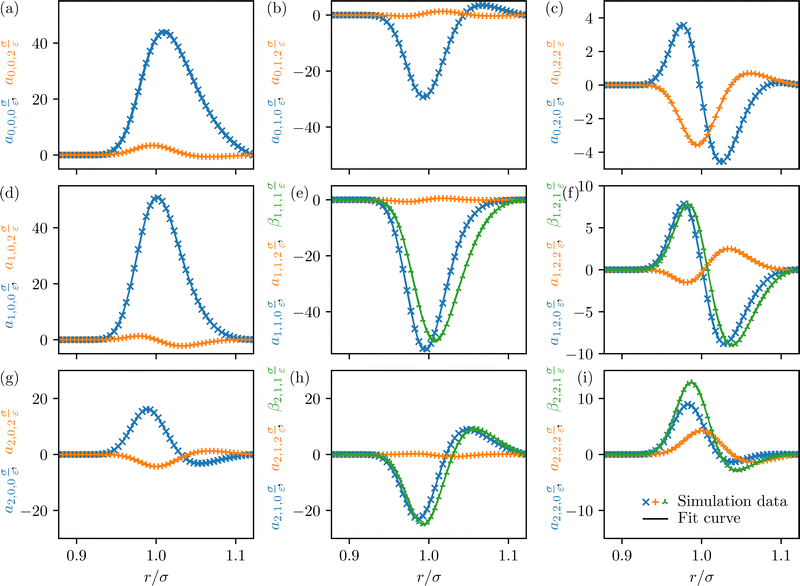
f2. The coefficients and their corresponding fits for Pe = 100 and
Φ0 = 0.2 are shown in
Fig. 9. We chose the fit function for each coefficient based on the number of zero-crossings and thus the required degree of the polynomial factor. As each coefficient also depends on the Péclet number and the packing density, the function to fit each coefficient is chosen according to the maximum number of zero-crossings observed for any value of Pe and
Φ0. If the number of zero-crossings changes with Pe or
Φ0, the roots of the polynomial term can move out of the interval, where
p is nonzero, causing numerical instability. These cases are treated separately with adjusted starting values for the fit to obtain reasonably smooth curves for the coefficients in Pe −
Φ0 parameter space.
 |
| | Fig. 9 Fourier coefficients αh,j,k(Pe, Φ0; r) and βh,j,1(Pe, Φ0; r) for the simulation data (symbols) and the corresponding fitted functions f0, f1, f2, f3, and f4 (solid lines) at the reference parameters Pe = 100 and Φ0 = 0.2. The coefficients αh,j,k and βh,j,1 are plotted in the h-th row and the j-th column. Coefficients where the last index is zero are plotted with blue crosses, while green triangular symbols are used for coefficients where the last index is one, and orange plus symbols are used if the last index is two. Since βh,j,k = 0 for h = 0 or j = 0, there are only two rather than three curves in (a), (b), (c), (d), and (g). | |
Table 1 Fit coefficients of the function h(Pe, Φ0) used to fit the variables of the Fourier coefficients α0,0,0, α0,0,2,th and α0,1,0 of the function p
|
|
q
−2,0
|
q
−2,1
|
q
−2,2
|
q
−2,3
|
q
−1,0
|
q
−1,1
|
q
−1,2
|
|
q
−1,3
|
q
0,0
|
q
0,1
|
q
0,2
|
q
0,3
|
q
1,0
|
q
1,1
|
|
q
1,2
|
q
1,3
|
q
2,0
|
q
2,1
|
q
2,2
|
q
2,3
|
|
α
0,0,0
via f
0
|
a
|
3.851 × 10³ |
−1.123 × 10³ |
1.455 × 10² |
−3.513 |
5.588 × 10⁻² |
−6.308 × 10⁴ |
2.123 × 10⁴ |
| −2.379 × 10³ |
1.222 × 10² |
−2.224 |
2.768 × 10⁵ |
−9.911 × 10⁴ |
1.235 × 10⁴ |
−6.949 × 10² |
| 1.387 × 101 |
−4.123 × 10⁵ |
1.561 × 10⁵ |
−2.077 × 10⁴ |
1.250 × 10³ |
−2.639 × 101 |
|
|
μ
|
−2.447 |
4.542 × 10⁻¹ |
9.584 × 10⁻¹ |
1.890 × 10⁻³ |
−3.198 × 10⁻⁵ |
2.386 × 101 |
−8.424 |
| 9.945 × 10⁻¹ |
−5.162 × 10⁻² |
9.456 × 10⁻⁴ |
−9.346 × 101 |
3.426 × 101 |
−4.336 |
2.438 × 10⁻¹ |
| −4.811 × 10⁻³ |
1.172 × 10² |
−4.404 × 101 |
5.750 |
−3.532 × 10⁻¹ |
7.436 × 10⁻³ |
|
|
ω
|
−2.809 × 10⁻¹ |
1.406 × 10⁻¹ |
1.862 × 10⁻² |
−1.068 × 10⁻³ |
2.083 × 10⁻⁵ |
−2.633 |
1.033 |
| −1.586 × 10⁻¹ |
1.068 × 10⁻² |
−2.284 × 10⁻⁴ |
2.100 × 101 |
−7.963 |
1.087 |
−6.189 × 10⁻² |
| 1.352 × 10⁻³ |
−4.072 × 101 |
1.581 × 101 |
−2.220 |
1.285 × 10⁻¹ |
−2.727 × 10⁻³ |
|
|
λ
|
−3.405 × 10² |
3.984 × 101 |
1.498 × 101 |
−6.157 × 10⁻¹ |
1.349 × 10⁻² |
−1.203 × 10³ |
3.853 × 10² |
| −3.356 × 101 |
1.403 |
−3.188 × 10⁻² |
2.147 × 10⁴ |
−7.477 × 10³ |
8.545 × 10² |
−3.612 × 101 |
| 5.803 × 10⁻¹ |
−4.258 × 10⁴ |
1.556 × 10⁴ |
−1.910 × 10³ |
9.345 × 101 |
−1.518 |
|
|
|
|
α
0,0,2
via f
1
|
a
|
2.002 × 10³ |
−1.673 × 10³ |
3.808 × 10² |
−2.512 × 101 |
1.068 |
−7.529 × 10³ |
1.430 × 10⁴ |
| −4.393 × 10³ |
4.686 × 10² |
−1.677 × 101 |
1.998 × 10⁵ |
−1.258 × 10⁵ |
2.746 × 10⁴ |
−2.472 × 10³ |
| 7.922 × 101 |
−5.533 × 10⁵ |
2.766 × 10⁵ |
−5.103 × 10⁴ |
4.068 × 10³ |
−1.196 × 10² |
|
|
μ
|
7.683 × 10⁻¹ |
−8.353 × 10⁻¹ |
1.131 |
−6.676 × 10⁻³ |
1.113 × 10⁻⁴ |
−3.965 × 10⁻¹ |
7.200 × 10⁻¹ |
| −2.385 × 10⁻¹ |
1.658 × 10⁻² |
−3.064 × 10⁻⁴ |
−1.126 × 101 |
3.394 |
−1.351 × 10⁻¹ |
1.328 × 10⁻³ |
| −2.613 × 10⁻⁵ |
6.032 |
−1.457 |
−1.526 × 10⁻¹ |
−7.083 × 10⁻³ |
3.552 × 10⁻⁴ |
|
|
ω
|
1.121 |
−3.779 × 10⁻¹ |
8.119 × 10⁻² |
−4.018 × 10⁻³ |
6.869 × 10⁻⁵ |
−1.637 × 101 |
6.245 |
| −8.541 × 10⁻¹ |
4.794 × 10⁻² |
−8.917 × 10⁻⁴ |
7.400 × 101 |
−2.869 × 101 |
3.968 |
−2.256 × 10⁻¹ |
| 4.411 × 10⁻³ |
−1.132 × 10² |
4.451 × 101 |
−6.264 |
3.627 × 10⁻¹ |
−7.212 × 10⁻³ |
|
|
λ
|
2.774 × 10³ |
−1.165 × 10³ |
1.764 × 10² |
−9.081 |
1.509 × 10⁻¹ |
−1.052 × 10⁴ |
3.676 × 10³ |
| −4.609 × 10² |
2.911 × 101 |
−4.903 × 10⁻¹ |
2.058 × 10⁴ |
−4.807 × 10³ |
2.294 × 10² |
−2.137 |
| −1.030 × 10⁻¹ |
−1.663 × 10⁴ |
2.009 × 10³ |
4.356 × 10² |
−4.623 × 101 |
1.114 |
|
|
b
|
−2.267 |
7.610 × 10⁻¹ |
9.643 × 10⁻¹ |
5.106 × 10⁻³ |
−7.955 × 10⁻⁵ |
2.320 × 101 |
−8.191 |
| 9.121 × 10⁻¹ |
−5.206 × 10⁻² |
8.520 × 10⁻⁴ |
−8.120 × 101 |
2.672 × 101 |
−3.146 |
1.709 × 10⁻¹ |
| −3.017 × 10⁻³ |
8.219 × 101 |
−2.691 × 101 |
3.089 |
−1.851 × 10⁻¹ |
3.605 × 10⁻³ |
|
|
|
|
α
0,1,0
via f
1
|
a
|
1.254 × 10⁴ |
−4.106 × 10³ |
4.094 × 10² |
−7.510 × 101 |
1.081 |
−6.389 × 10⁵ |
2.173 × 10⁵ |
| −2.288 × 10⁴ |
8.477 × 10² |
−7.028 |
2.438 × 10⁶ |
−8.023 × 10⁵ |
8.265 × 10⁴ |
−3.102 × 10³ |
| 1.588 × 101 |
−2.316 × 10⁶ |
7.385 × 10⁵ |
−7.197 × 10⁴ |
2.339 × 10³ |
1.562 × 101 |
|
|
μ
|
−1.037 |
−1.579 × 10⁻¹ |
1.038 |
−2.019 × 10⁻³ |
3.411 × 10⁻⁵ |
1.358 × 101 |
−4.490 |
| 4.320 × 10⁻¹ |
−1.802 × 10⁻² |
2.691 × 10⁻⁴ |
−4.949 × 101 |
1.729 × 101 |
−1.811 |
8.411 × 10⁻² |
| −1.360 × 10⁻³ |
3.676 × 101 |
−1.206 × 101 |
1.014 |
−5.802 × 10⁻² |
1.081 × 10⁻³ |
|
|
ω
|
1.481 × 10⁻¹ |
−3.711 × 10⁻² |
3.976 × 10⁻² |
−2.111 × 10⁻³ |
3.894 × 10⁻⁵ |
−7.839 |
3.182 |
| −4.780 × 10⁻¹ |
2.936 × 10⁻² |
−5.927 × 10⁻⁴ |
4.763 × 101 |
−1.909 × 101 |
2.778 |
−1.651 × 10⁻¹ |
| 3.408 × 10⁻³ |
−8.552 × 101 |
3.435 × 101 |
−4.986 |
2.964 × 10⁻¹ |
−6.075 × 10⁻³ |
|
|
λ
|
2.346 × 10³ |
−9.704 × 10² |
1.326 × 10² |
−5.178 |
7.707 × 10⁻² |
−6.794 × 10³ |
1.505 × 10³ |
| −1.468 × 101 |
−4.196 |
1.692 × 10⁻¹ |
−1.182 × 10³ |
5.812 × 10³ |
−1.582 × 10³ |
1.183 × 10² |
| −2.453 |
2.176 × 10⁴ |
−1431 × 104 |
2.889 × 10³ |
−1.957 × 10² |
3.904 |
|
|
b
|
−1.483 |
1.184 |
8.966 × 10⁻¹ |
8.901 × 10⁻³ |
−1.679 × 10⁻⁴ |
3.249 × 101 |
−1.538 × 101 |
| 2.104 |
−1.287 × 10⁻¹ |
2.594 × 10⁻³ |
−1.586 × 10² |
6.435 × 101 |
−9.404 |
5.762 × 10⁻¹ |
| −1.212 × 10⁻² |
2.251 × 10² |
−8.935 × 101 |
1.304 × 101 |
−8.239 × 10⁻¹ |
1.778 × 10⁻² |
|
Table 2 Table of fit coefficients analog to Table 1, but for the Fourier coefficients α0,1,2, α0,2,0, and α0,2,2
|
|
q
−2,0
|
q
−2,1
|
q
−2,2
|
q
−2,3
|
q
−1,0
|
q
−1,1
|
q
−1,2
|
|
q
−1,3
|
q
0,0
|
q
0,1
|
q
0,2
|
q
0,3
|
q
1,0
|
q
1,1
|
|
q
1,2
|
q
1,3
|
q
2,0
|
q
2,1
|
q
2,2
|
q
2,3
|
|
α
0,1,2
via f
2
|
a
|
3.634 × 10⁵ |
−1.563 × 10⁵ |
2.507 × 10⁴ |
−1.702 × 10³ |
2.754 × 101 |
−4.355 × 10⁶ |
1.626 × 10⁶ |
| −2.133 × 10⁵ |
1.126 × 10⁴ |
−1.742 × 10² |
1.759 × 10⁷ |
−6.411 × 10⁶ |
8.051 × 10⁵ |
−3.937 × 10⁴ |
| 5.723 × 10² |
−2.229 × 10⁷ |
8.150 × 10⁶ |
−1.024 × 10⁶ |
4.955 × 10⁴ |
−6.691 × 10² |
|
|
μ
|
3.288 × 10⁻¹ |
−7.811 × 10⁻¹ |
1.130 |
−6.010 × 10⁻³ |
9.349 × 10⁻⁵ |
3.024 |
1.652 |
| −5.221 × 10⁻¹ |
3.591 × 10⁻² |
−7.273 × 10⁻⁴ |
7.342 × 10⁻¹ |
−1.021 × 101 |
2.525 |
−1.780 × 10⁻¹ |
| 3.892 × 10⁻³ |
−1.064 × 101 |
1.781 × 101 |
−4.221 |
2.888 × 10⁻¹ |
−6.374 × 10⁻³ |
|
|
ω
|
9.646 × 10⁻¹ |
−3.793 × 10⁻¹ |
8.727 × 10⁻² |
−4.504 × 10⁻³ |
8.132 × 10⁻⁵ |
−1.558 × 101 |
7.503 |
| −1.171 |
7.068 × 10⁻² |
−1.411 × 10⁻³ |
8.686 × 101 |
−4.037 × 101 |
6.247 |
−3.791 × 10⁻¹ |
| 7.760 × 10⁻³ |
−1.444 × 10² |
6.508 × 101 |
−9.983 |
6.094 × 10⁻¹ |
−1.254 × 10⁻² |
|
|
λ
|
6.316 × 10³ |
−2.400 × 10³ |
3.151 × 10² |
−1.421 × 101 |
2.260 × 10⁻¹ |
−5.501 × 10⁴ |
1.956 × 10⁴ |
| −2.321 × 10³ |
1.177 × 10² |
−1.976 |
2.247 × 10⁵ |
−7.672 × 10⁴ |
8.659 × 10³ |
−4.104 × 10² |
| 6.932 |
−2.591 × 10⁵ |
8.718 × 10⁴ |
−9.476 × 10³ |
4.408 × 10² |
−7.454 |
|
|
b
|
−1.511 |
5.745 × 10⁻¹ |
1.010 |
3.445 × 10⁻³ |
−5.265 × 10⁻⁵ |
−3.274 |
2.234 × 10⁻¹ |
| −8.674 × 10⁻² |
−3.234 × 10⁻³ |
7.194 × 10⁻⁵ |
4.399 × 101 |
−1.757 × 101 |
2.111 |
−9.365 × 10⁻² |
| 1.354 × 10⁻³ |
−8.009 × 101 |
3.300 × 101 |
−4.349 |
2.017 × 10⁻¹ |
−3.030 × 10⁻³ |
|
|
c
|
−8.908 × 10⁻¹ |
−3.613 × 10⁻¹ |
1.043 |
−1.774 × 10⁻⁴ |
−1.274 × 10⁻⁵ |
−4.553 |
9.712 × 10⁻¹ |
| −1.633 × 10⁻² |
−1.058 × 10⁻² |
3.663 × 10⁻⁴ |
4.332 × 101 |
−1.122 × 101 |
4.903 × 10⁻¹ |
3.005 × 10⁻² |
| −1.496 × 10⁻³ |
−7.762 × 101 |
2.074 × 101 |
−1.261 |
−3.947 × 10⁻² |
2.319 × 10⁻³ |
|
|
|
|
α
0,2,0
via f
3
|
a
|
4.208 × 10⁴ |
4.401 × 10⁴ |
−1.751 × 10⁴ |
1.913 × 10³ |
−2.300 × 101 |
−4.087 × 10⁶ |
1.461 × 10⁶ |
| −1.860 × 10⁵ |
9.506 × 10³ |
−2.369 × 10² |
1.168 × 10⁷ |
−4.350 × 10⁶ |
5.895 × 10⁵ |
−3.447 × 10⁴ |
| 8.624 × 10² |
−3.928 × 10⁶ |
1.287 × 10⁶ |
−1.634 × 10⁵ |
1.205 × 10⁴ |
−5.759 × 10² |
|
|
μ
|
−1.690 |
−6.248 × 10⁻³ |
1.026 |
−1.100 × 10⁻³ |
1.390 × 10⁻⁵ |
3.729 × 101 |
−1.064 × 101 |
| 9.829 × 10⁻¹ |
−3.905 × 10⁻² |
5.705 × 10⁻⁴ |
−1.389 × 10² |
3.727 × 101 |
−3.208 |
1.113 × 10⁻¹ |
| −1.300 × 10⁻³ |
8.590 × 101 |
−1.522 × 101 |
−6.744 × 10⁻² |
6.539 × 10⁻² |
−2.028 × 10⁻³ |
|
|
ω
|
7.821 × 10⁻¹ |
−2.768 × 10⁻¹ |
6.939 × 10⁻² |
−3.540 × 10⁻³ |
6.355 × 10⁻⁵ |
−1.957 × 101 |
7.889 |
| −1.097 |
6.180 × 10⁻² |
−1.180 × 10⁻³ |
1.093 × 10² |
−4.394 × 101 |
6.069 |
−3.401 × 10⁻¹ |
| 6.590 × 10⁻³ |
−1.803 × 10² |
7.157 × 101 |
−9.904 |
5.593 × 10⁻¹ |
−1.086 × 10⁻² |
|
|
λ
|
−2.303 × 10⁴ |
7.985 × 10³ |
−9.645 × 10² |
5.099 × 101 |
−9.222 × 10⁻¹ |
4.980 × 10⁵ |
−1.760 × 10⁵ |
| 2.150 × 10⁴ |
−1.083 × 10³ |
1.928 × 101 |
−2.302 × 10⁶ |
8.174 × 10⁵ |
−1.004 × 10⁵ |
5.095 × 10³ |
| −9.095 × 101 |
2.942 × 10⁶ |
−1.049 × 10⁶ |
1.298 × 10⁵ |
−6.620 × 10³ |
1.187 × 10² |
|
|
b
|
−1.409 |
2.211 |
−2.499 |
2.368 × 10⁻² |
−4.594 × 10⁻⁴ |
7.873 × 101 |
−5.234 × 101 |
| 8.004 |
−4.453 × 10⁻¹ |
8.424 × 10⁻³ |
−5.396 × 10² |
2.802 × 10² |
−3.941 × 101 |
2.172 |
| −4.071 × 10⁻² |
8.501 × 10² |
−4.006 × 10² |
5.566 × 101 |
−3.036 |
5.698 × 10⁻² |
|
|
c
|
2.433 |
−2.558 |
1.539 |
−2.547 × 10⁻² |
4.896 × 10⁻⁴ |
−9.941 × 101 |
5.830 × 101 |
| −8.642 |
4.750 × 10⁻¹ |
−8.933 × 10⁻³ |
6.305 × 10² |
−3.061 × 10² |
4.217 × 101 |
−2.303 |
| 4.299 × 10⁻² |
−9.639 × 10² |
4.337 × 10² |
−5.922 × 101 |
3.208 |
−6.003 × 10⁻² |
|
|
|
|
α
0,2,2
via f
1
|
a
|
6.406 × 10³ |
−3.409 × 10³ |
6.365 × 10² |
−5.410 × 101 |
8.583 × 10⁻¹ |
−4.458 × 10⁴ |
2.302 × 10⁴ |
| −3.997 × 10³ |
2.663 × 10² |
−3.995 |
1.287 × 10⁵ |
−5.600 × 10⁴ |
8.468 × 10³ |
−5.111 × 10² |
| 6.340 |
−9.041 × 10⁴ |
3.268 × 10⁴ |
−3.920 × 10³ |
1.765 × 10² |
1.496 |
|
|
μ
|
−2.877 × 10⁻¹ |
−4.663 × 10⁻¹ |
1.073 |
−2.072 × 10⁻³ |
2.446 × 10⁻⁵ |
6.643 |
−4.170 × 10⁻² |
| −3.346 × 10⁻¹ |
2.613 × 10⁻² |
−5.736 × 10⁻⁴ |
−7.125 |
−6.820 |
2.375 |
−1.891 × 10⁻¹ |
| 4.291 × 10⁻³ |
−4.730 × 101 |
2.915 × 101 |
−5.767 |
3.856 × 10⁻¹ |
−8.336 × 10⁻³ |
|
|
ω
|
2.438 × 10⁻¹ |
−9.165 × 10⁻² |
4.796 × 10⁻² |
−2.486 × 10⁻³ |
4.870 × 10⁻⁵ |
−1.656 × 101 |
7.057 |
| −1.055 |
6.350 × 10⁻² |
−1.283 × 10⁻³ |
1.012 × 10² |
−4.176 × 101 |
6.105 |
−3.644 × 10⁻¹ |
| 7.443 × 10⁻³ |
−1.677 × 10² |
6.831 × 101 |
−9.932 |
5.939 × 10⁻¹ |
−1.213 × 10⁻² |
|
|
λ
|
3.832 × 10³ |
−1.407 × 10³ |
1.569 × 10² |
−2.707 |
−5.794 × 10⁻³ |
−3.534 × 10⁴ |
1.550 × 10⁴ |
| −2.290 × 10³ |
1.322 × 10² |
−2.333 |
1.628 × 10⁵ |
−7.364 × 10⁴ |
1.161 × 10⁴ |
−7.420 × 10² |
| 1.487 × 101 |
−2.613 × 10⁵ |
1.148 × 10⁵ |
−1.784 × 10⁴ |
1.153 × 10³ |
−2.415 × 101 |
|
|
b
|
−2.331 |
1.006 |
9.082 × 10⁻¹ |
6.947 × 10⁻³ |
−1.271 × 10⁻⁴ |
2.035 × 101 |
−9.455 |
| 1.407 |
−8.407 × 10⁻² |
1.647 × 10⁻³ |
−8.484 × 101 |
3.532 × 101 |
−5.382 |
3.332 × 10⁻¹ |
| −6.790 × 10⁻³ |
1.136 × 10² |
−4.555 × 101 |
6.634 |
−4.295 × 10⁻¹ |
8.994 × 10⁻³ |
|
Table 3 Table of fit coefficients analog to Table 1, but for the Fourier coefficients α1,0,0, α1,0,2, and α1,1,0
|
|
q
−2,0
|
q
−2,1
|
q
−2,2
|
q
−2,3
|
q
−1,0
|
q
−1,1
|
q
−1,2
|
|
q
−1,3
|
q
0,0
|
q
0,1
|
q
0,2
|
q
0,3
|
q
1,0
|
q
1,1
|
|
q
1,2
|
q
1,3
|
q
2,0
|
q
2,1
|
q
2,2
|
q
2,3
|
|
α
1,0,0
via f
1
|
a
|
3.223 × 10⁴ |
−2.288 × 10³ |
6.567 × 10² |
1.037 × 101 |
−3.946 × 10⁻¹ |
1.926 × 10⁵ |
−7.301 × 10⁴ |
| 4.908 × 10³ |
−5.720 × 101 |
2.264 × 10⁻² |
−6.046 × 10⁵ |
9.449 × 10⁴ |
9.811 × 10³ |
−1.600 × 10³ |
| 3.774 × 101 |
−3.533 × 10⁵ |
3.060 × 10⁵ |
−6.497 × 10⁴ |
4.935 × 10³ |
−1.050 × 10² |
|
|
μ
|
−2.140 |
2.843 × 10⁻¹ |
9.816 × 10⁻¹ |
6.331 × 10⁻⁴ |
−8.452 × 10⁻⁶ |
1.917 × 101 |
−6.149 |
| 6.120 × 10⁻¹ |
−2.679 × 10⁻² |
4.236 × 10⁻⁴ |
−6.004 × 101 |
1.915 × 101 |
−1.922 |
8.518 × 10⁻² |
| −1.418 × 10⁻³ |
4.008 × 101 |
−1.128 × 101 |
7.895 × 10⁻¹ |
−3.938 × 10⁻² |
8.041 × 10⁻⁴ |
|
|
ω
|
−2.134 × 10⁻¹ |
9.436 × 10⁻² |
2.385 × 10⁻² |
−1.383 × 10⁻³ |
2.739 × 10⁻⁵ |
−5.739 |
2.502 |
| −3.917 × 10⁻¹ |
2.467 × 10⁻² |
−5.049 × 10⁻⁴ |
4.312 × 101 |
−1.769 × 101 |
2.575 |
−1.528 × 10⁻¹ |
| 3.144 × 10⁻³ |
−8.246 × 101 |
3.333 × 101 |
−4.815 |
2.852 × 10⁻¹ |
−5.814 × 10⁻³ |
|
|
λ
|
3.563 × 10² |
−2.105 × 10² |
3.310 × 101 |
−1.076 |
2.070 × 10⁻² |
2.838 × 10³ |
−1.121 × 10³ |
| 1.430 × 10² |
−4.706 |
2.109 × 10⁻² |
7.034 × 10³ |
−2.198 × 10³ |
2.767 × 10² |
−1.819 × 101 |
| 5.701 × 10⁻¹ |
−4.452 × 10⁴ |
1.665 × 10⁴ |
−2.183 × 10³ |
1.247 × 10² |
−2.551 |
|
|
b
|
2.516 |
−7.562 × 10⁻¹ |
1.193 |
−3.130 × 10⁻³ |
5.917 × 10⁻⁵ |
−3.627 × 101 |
1.175 × 101 |
| −1.119 |
3.478 × 10⁻² |
−5.025 × 10⁻⁴ |
5.457 × 101 |
−1.370 × 101 |
3.540 × 10⁻¹ |
4.920 × 10⁻² |
| −1.397 × 10⁻³ |
3.410 × 101 |
−1.994 × 101 |
3.682 |
−2.765 × 10⁻¹ |
5.581 × 10⁻³ |
|
|
|
|
α
1,0,2
via f
2
|
a
|
−6.856 × 10⁵ |
2.623 × 10⁵ |
−3.660 × 10⁴ |
2.245 × 10³ |
−3.185 × 101 |
6.137 × 10⁶ |
−2.170 × 10⁶ |
| 2.585 × 10⁵ |
−1.155 × 10⁴ |
7.410 × 101 |
−1.449 × 10⁷ |
4.651 × 10⁶ |
−4.465 × 10⁵ |
8.896 × 10³ |
| 4.563 × 10² |
7.552 × 10⁶ |
−1.681 × 10⁶ |
−2.437 × 10⁴ |
2.417 × 10⁴ |
−1.310 × 10³ |
|
|
μ
|
2.029 |
−1.334 |
1.200 |
−1.022 × 10⁻² |
1.755 × 10⁻⁴ |
−2.053 × 101 |
9.209 |
| −1.457 |
8.576 × 10⁻² |
−1.652 × 10⁻³ |
1.027 × 10² |
−4.345 × 101 |
6.565 |
−3.852 × 10⁻¹ |
| 7.595 × 10⁻³ |
−1.842 × 10² |
7.522 × 101 |
−1.102 × 101 |
6.226 × 10⁻¹ |
−1.209 × 10⁻² |
|
|
ω
|
1.211 |
−4.355 × 10⁻¹ |
9.142 × 10⁻² |
−4.701 × 10⁻³ |
8.333 × 10⁻⁵ |
−1.655 × 101 |
6.928 |
| −1.013 |
5.926 × 10⁻² |
−1.150 × 10⁻³ |
8.318 × 101 |
−3.464 × 101 |
5.056 |
−2.970 × 10⁻¹ |
| 5.950 × 10⁻³ |
−1.396 × 10² |
5.726 × 101 |
−8.294 |
4.881 × 10⁻¹ |
−9.797 × 10⁻³ |
|
|
λ
|
3.516 × 10³ |
−1.375 × 10³ |
1.888 × 10² |
−9.350 |
1.590 × 10⁻¹ |
−1.693 × 10⁴ |
5.801 × 10³ |
| −6.929 × 10² |
3.810 × 101 |
−6.390 × 10⁻¹ |
4.885 × 10⁴ |
−1.419 × 10⁴ |
1.327 × 10³ |
−4.528 × 101 |
| 5.316 × 10⁻¹ |
−5.412 × 10⁴ |
1.444 × 10⁴ |
−1.023 × 10³ |
1.249 × 101 |
2.942 × 10⁻¹ |
|
|
b
|
9.896 × 10⁻¹ |
−5.359 × 10⁻¹ |
1.211 |
−6.517 × 10⁻³ |
1.397 × 10⁻⁴ |
−2.115 × 101 |
1.078 × 101 |
| −1.550 |
8.464 × 10⁻² |
−1.658 × 10⁻³ |
5.515 × 101 |
−3.271 × 101 |
4.342 |
−2.490 × 10⁻¹ |
| 4.841 × 10⁻³ |
−3.356 × 101 |
2.410 × 101 |
−3.469 |
1.856 × 10⁻¹ |
−3.718 × 10⁻³ |
|
|
c
|
−1.102 |
−9.582 × 10⁻² |
1.031 |
5.216 × 10⁻⁴ |
−2.164 × 10⁻⁵ |
1.656 × 101 |
−6.405 |
| 8.220 × 10⁻¹ |
−5.035 × 10⁻² |
1.016 × 10⁻³ |
−9.621 × 101 |
3.594 × 101 |
−4.997 |
2.923 × 10⁻¹ |
| −5.857 × 10⁻³ |
1.464 × 10² |
−5.501 × 101 |
7.618 |
−4.640 × 10⁻¹ |
9.416 × 10⁻³ |
|
|
|
|
α
1,1,0
via f
1
|
a
|
−8.518 × 10⁴ |
2.794 × 10⁴ |
−3.583 × 10³ |
1.440 × 10² |
−3.291 |
1.474 × 10⁶ |
−6.368 × 10⁵ |
| 9.604 × 10⁴ |
−5.886 × 10³ |
1.252 × 10² |
−8.437 × 10⁶ |
3.705 × 10⁶ |
−5.728 × 10⁵ |
3.648 × 10⁴ |
| −7.875 × 10² |
1.506 × 10⁷ |
−6.437 × 10⁶ |
9.829 × 10⁵ |
−6.297 × 10⁴ |
1.383 × 10³ |
|
|
μ
|
−9.903 × 10⁻¹ |
−1.304 × 10⁻¹ |
1.026 |
−1.183 × 10⁻³ |
1.950 × 10⁻⁵ |
2.422 × 101 |
−7.403 |
| 6.854 × 10⁻¹ |
−2.596 × 10⁻² |
3.136 × 10⁻⁴ |
−9.704 × 101 |
3.082 × 101 |
−3.044 |
1.126 × 10⁻¹ |
| −1.177 × 10⁻³ |
8.049 × 101 |
−2.415 × 101 |
1.997 |
−5.759 × 10⁻² |
−1.402 × 10⁻⁴ |
|
|
ω
|
2.283 × 10⁻¹ |
−6.643 × 10⁻² |
4.315 × 10⁻² |
−2.368 × 10⁻³ |
4.591 × 10⁻⁵ |
−9.536 |
4.169 |
| −6.508 × 10⁻¹ |
4.102 × 10⁻² |
−8.558 × 10⁻⁴ |
6.041 × 101 |
−2.522 × 101 |
3.767 |
−2.315 × 10⁻¹ |
| 4.892 × 10⁻³ |
−1.094 × 10² |
4.471 × 101 |
−6.566 |
3.996 × 10⁻¹ |
−8.359 × 10⁻³ |
|
|
λ
|
2.680 × 10² |
1.972 × 101 |
−4.234 × 101 |
7.669 |
−2.021 × 10⁻¹ |
1.199 × 10⁵ |
−4.799 × 10⁴ |
| 6.796 × 10³ |
−3.944 × 10² |
7.966 |
−7.647 × 10⁵ |
3.076 × 10⁵ |
−4.395 × 10⁴ |
2.588 × 10³ |
| −5.229 × 101 |
1.235 × 10⁶ |
−4.997 × 10⁵ |
7.238 × 10⁴ |
−4.362 × 10³ |
9.052 × 101 |
|
|
b
|
−1.006 × 101 |
4.058 |
5.726 × 10⁻¹ |
2.575 × 10⁻² |
−5.068 × 10⁻⁴ |
6.333 × 101 |
−3.497 × 101 |
| 6.370 |
−4.427 × 10⁻¹ |
1.021 × 10⁻² |
−4.339 × 10² |
2.164 × 10² |
−3.776 × 101 |
2.670 |
| −6.371 × 10⁻² |
8.827 × 10² |
−4.060 × 10² |
6.701 × 101 |
−4.706 |
1.154 × 10⁻¹ |
|
Table 4 Table of fit coefficients analog to Table 1, but for the Fourier coefficients α1,1,2, α1,2,0, and α1,2,2
|
|
q
−2,0
|
q
−2,1
|
q
−2,2
|
q
−2,3
|
q
−1,0
|
q
−1,1
|
q
−1,2
|
|
q
−1,3
|
q
0,0
|
q
0,1
|
q
0,2
|
q
0,3
|
q
1,0
|
q
1,1
|
|
q
1,2
|
q
1,3
|
q
2,0
|
q
2,1
|
q
2,2
|
q
2,3
|
|
α
1,1,2
via f
4
|
a
|
−9.954 × 10⁵ |
2.120 × 10⁵ |
1.642 × 10⁴ |
−3.131 × 10³ |
−2.341 × 10² |
6.628 × 10⁷ |
−3.079 × 10⁷ |
| 4.842 × 10⁶ |
−3.063 × 10⁵ |
7.906 × 10³ |
−2.906 × 10⁸ |
1.332 × 10⁸ |
−2.123 × 10⁷ |
1.364 × 10⁶ |
| −3.168 × 10⁴ |
3.307 × 10⁸ |
−1.482 × 10⁸ |
2.346 × 10⁷ |
−1.508 × 10⁶ |
3.412 × 10⁴ |
|
|
μ
|
2.706 × 101 |
−8.866 |
1.981 |
−4.382 × 10⁻² |
6.967 × 10⁻⁴ |
−5.583 × 10² |
1.683 × 10² |
| −1.796 × 101 |
8.070 × 10⁻¹ |
−1.299 × 10⁻² |
2.507 × 10³ |
−7.586 × 10² |
8.095 × 101 |
−3.643 |
| 5.881 × 10⁻² |
−2.676 × 10³ |
8.214 × 10² |
−8.910 × 101 |
4.054 |
−6.591 × 10⁻² |
|
|
ω
|
−1.849 |
5.386 × 10⁻¹ |
−1.905 × 10⁻² |
5.845 × 10⁻⁴ |
−6.065 × 10⁻⁶ |
1.305 × 101 |
−3.052 |
| 1.179 × 10⁻¹ |
5.620 × 10⁻³ |
−2.471 × 10⁻⁴ |
6.669 × 101 |
−2.891 × 101 |
4.476 |
−2.723 × 10⁻¹ |
| 5.539 × 10⁻³ |
−3.221 × 10² |
1.182 × 10² |
−1.548 × 101 |
8.384 × 10⁻¹ |
−1.575 × 10⁻² |
|
|
λ
|
−1.544 × 10⁴ |
4.235 × 10³ |
−3.744 × 10² |
1.519 × 101 |
−2.225 × 10⁻¹ |
2.254 × 10⁵ |
−6.849 × 10⁴ |
| 6.548 × 10³ |
−2.482 × 10² |
3.383 |
−3.195 × 10⁵ |
1.059 × 10⁵ |
−8.572 × 10³ |
2.122 × 10² |
| −7.060 × 10⁻¹ |
−2.433 × 10⁴ |
−2.159 × 10³ |
−2.794 × 10³ |
3.278 × 10² |
−8.104 |
|
|
b
|
−2.534 × 10² |
7.861 × 101 |
−1.061 × 101 |
3.801 × 10⁻¹ |
−6.141 × 10⁻³ |
4.491 × 10³ |
−1.408 × 10³ |
| 1.520 × 10² |
−6.850 |
1.107 × 10⁻¹ |
−1.878 × 10⁴ |
5.946 × 10³ |
−6.453 × 10² |
2.919 × 101 |
| −4.724 × 10⁻¹ |
1.924 × 10⁴ |
−6.144 × 10³ |
6.728 × 10² |
−3.056 × 101 |
4.967 × 10⁻¹ |
|
|
c
|
2.774 × 10² |
−8.556 × 101 |
1.032 × 101 |
−4.104 × 10⁻¹ |
6.609 × 10⁻³ |
−4.936 × 10³ |
1.539 × 10³ |
| −1.653 × 10² |
7.422 |
−1.195 × 10⁻¹ |
2.064 × 10⁴ |
−6.495 × 10³ |
7.012 × 10² |
−3.158 × 101 |
| 5.093 × 10⁻¹ |
−2.112 × 10⁴ |
6.694 × 10³ |
−7.280 × 10² |
3.288 × 101 |
−5.318 × 10⁻¹ |
|
|
d
|
5.807 |
−2.391 |
1.279 |
−1.231 × 10⁻² |
2.048 × 10⁻⁴ |
−9.335 × 101 |
3.723 × 101 |
| −4.730 |
2.371 × 10⁻¹ |
−4.149 × 10⁻³ |
4.002 × 10² |
−1.624 × 10² |
2.128 × 101 |
−1.100 |
| 1.957 × 10⁻² |
−5.175 × 10² |
2.080 × 10² |
−2.763 × 101 |
1.440 |
−2.580 × 10⁻² |
|
|
|
|
α
1,2,0
via f
2
|
a
|
−1.603 × 10⁶ |
5.281 × 10⁵ |
−6.178 × 10⁴ |
3.512 × 10³ |
−3.307 × 101 |
1.316 × 10⁷ |
−3.828 × 10⁶ |
| 3.396 × 10⁵ |
−1.020 × 10⁴ |
−4.895 × 101 |
−3.643 × 10⁷ |
1.044 × 10⁷ |
−8.937 × 10⁵ |
2.292 × 10⁴ |
| 2.179 × 10² |
3.757 × 10⁷ |
−1.153 × 10⁷ |
1.135 × 10⁶ |
−3.984 × 10⁴ |
1.086 × 10² |
|
|
μ
|
−2.224 × 10⁻¹ |
−3.805 × 10⁻¹ |
1.058 |
−2.449 × 10⁻³ |
3.693 × 10⁻⁵ |
2.086 |
−1.258 × 10⁻¹ |
| −1.434 × 10⁻¹ |
1.218 × 10⁻² |
−2.771 × 10⁻⁴ |
1.015 × 101 |
−6.481 |
1.503 |
−1.069 × 10⁻¹ |
| 2.338 × 10⁻³ |
−6.222 × 101 |
2.774 × 101 |
−4.642 |
2.769 × 10⁻¹ |
−5.567 × 10⁻³ |
|
|
ω
|
4.124 × 10⁻¹ |
−1.154 × 10⁻¹ |
4.686 × 10⁻² |
−2.377 × 10⁻³ |
4.308 × 10⁻⁵ |
−1.404 × 101 |
5.388 |
| −7.470 × 10⁻¹ |
4.257 × 10⁻² |
−8.198 × 10⁻⁴ |
7.506 × 101 |
−2.902 × 101 |
4.028 |
−2.294 × 10⁻¹ |
| 4.514 × 10⁻³ |
−1.146 × 10² |
4.511 × 101 |
−6.376 |
3.700 × 10⁻¹ |
−7.320 × 10⁻³ |
|
|
λ
|
9.843 × 10² |
−3.044 × 10² |
1.410 × 101 |
3.312 |
−8.335 × 10⁻² |
3.068 × 10⁴ |
−1.097 × 10⁴ |
| 1.377 × 10³ |
−7.070 × 101 |
1.315 |
−1.387 × 10⁵ |
4.859 × 10⁴ |
−5.797 × 10³ |
2.768 × 10² |
| −4.606 |
1.294 × 10⁵ |
−4.443 × 10⁴ |
5.192 × 10³ |
−2.296 × 10² |
3.289 |
|
|
b
|
−1.178 |
8.993 × 10⁻² |
9.996 × 10⁻¹ |
1.577 × 10⁻³ |
−4.047 × 10⁻⁵ |
1.308 × 101 |
−5.517 |
| 8.110 × 10⁻¹ |
−5.199 × 10⁻² |
1.105 × 10⁻³ |
−8.077 × 101 |
3.134 × 101 |
−4.710 |
2.929 × 10⁻¹ |
| −6.156 × 10⁻³ |
1.276 × 10² |
−4.931 × 101 |
7.152 |
−4.577 × 10⁻¹ |
9.653 × 10⁻³ |
|
|
c
|
1.477 × 101 |
−4.696 |
1.599 |
−2.106 × 10⁻² |
2.870 × 10⁻⁴ |
−1.491 × 10² |
4.808 × 101 |
| −4.498 |
1.570 × 10⁻¹ |
−1.685 × 10⁻³ |
3.277 × 10² |
−1.025 × 10² |
8.055 |
−1.884 × 10⁻¹ |
| 1.196 × 10⁻⁴ |
−1.812 × 10² |
5.169 × 101 |
−2.704 |
−7.203 × 10⁻² |
3.840 × 10⁻³ |
|
|
|
|
α
1,2,2
via f
2
|
a
|
1.995 × 10⁵ |
−4.584 × 10⁴ |
2.683 × 10³ |
−6.353 × 101 |
−1.861 × 101 |
−9.766 × 10⁵ |
−5.245 × 10⁴ |
| 7.792 × 10⁴ |
−9.151 × 10³ |
3.511 × 10² |
4.686 × 10⁵ |
1.249 × 10⁶ |
−4.199 × 10⁵ |
4.196 × 10⁴ |
| −1.398 × 10³ |
2.044 × 10⁶ |
−2.260 × 10⁶ |
5.774 × 10⁵ |
−5.380 × 10⁴ |
1.740 × 10³ |
|
|
μ
|
−1.569 |
1.049 × 10⁻¹ |
9.985 × 10⁻¹ |
1.772 × 10⁻³ |
−4.592 × 10⁻⁵ |
1.083 × 101 |
−4.147 |
| 4.547 × 10⁻¹ |
−2.317 × 10⁻² |
4.135 × 10⁻⁴ |
2.323 |
1.119 |
4.159 × 10⁻² |
−1.229 × 10⁻² |
| 4.499 × 10⁻⁴ |
−6.955 × 101 |
2.414 × 101 |
−3.515 |
1.915 × 10⁻¹ |
−3.820 × 10⁻³ |
|
|
ω
|
−3.021 × 10⁻¹ |
1.531 × 10⁻¹ |
1.326 × 10⁻² |
−5.701 × 10⁻⁴ |
1.048 × 10⁻⁵ |
−1.368 × 101 |
4.801 |
| −6.378 × 10⁻¹ |
3.622 × 10⁻² |
−7.034 × 10⁻⁴ |
1.036 × 10² |
−3.659 × 101 |
4.755 |
−2.609 × 10⁻¹ |
| 5.072 × 10⁻³ |
−1.736 × 10² |
6.276 × 101 |
−8.296 |
4.611 × 10⁻¹ |
−8.971 × 10⁻³ |
|
|
λ
|
−2.170 × 10² |
2.196 × 10² |
−6.125 × 101 |
7.196 |
−1.708 × 10⁻¹ |
1.436 × 10⁴ |
−5.802 × 10³ |
| 8.287 × 10² |
−4.758 × 101 |
1.017 |
−5.956 × 10⁴ |
2.262 × 10⁴ |
−2.840 × 10³ |
1.426 × 10² |
| −2.497 |
4.964 × 10⁴ |
−1.922 × 10⁴ |
2.423 × 10³ |
−1.088 × 10² |
1.442 |
|
|
b
|
9.771 |
−3.248 |
1.504 |
−1.990 × 10⁻² |
3.215 × 10⁻⁴ |
−1.267 × 10² |
4.251 × 101 |
| −4.779 |
2.194 × 10⁻¹ |
−3.474 × 10⁻³ |
3.875 × 10² |
−1.322 × 10² |
1.429 × 101 |
−6.451 × 10⁻¹ |
| 1.002 × 10⁻² |
−3.313 × 10² |
1.128 × 10² |
−1.223 × 101 |
5.206 × 10⁻¹ |
−7.804 × 10⁻³ |
|
|
c
|
−9.916 × 10⁻¹ |
−8.805 × 10⁻² |
1.027 |
9.428 × 10⁻⁴ |
−2.910 × 10⁻⁵ |
1.123 × 101 |
−5.418 |
| 7.821 × 10⁻¹ |
−4.997 × 10⁻² |
1.038 × 10⁻³ |
−7.815 × 101 |
3.260 × 101 |
−4.908 |
2.965 × 10⁻¹ |
| −6.045 × 10⁻³ |
1.262 × 10² |
−5.084 × 101 |
7.453 |
−4.679 × 10⁻¹ |
9.577 × 10⁻³ |
|
Table 5 Table of fit coefficients analog to Table 1, but for the Fourier coefficients α2,0,0, α2,0,2, and α2,1,0
|
|
q
−2,0
|
q
−2,1
|
q
−2,2
|
q
−2,3
|
q
−1,0
|
q
−1,1
|
q
−1,2
|
|
q
−1,3
|
q
0,0
|
q
0,1
|
q
0,2
|
q
0,3
|
q
1,0
|
q
1,1
|
|
q
1,2
|
q
1,3
|
q
2,0
|
q
2,1
|
q
2,2
|
q
2,3
|
|
α
2,0,0
via f
1
|
a
|
2.232 × 10⁴ |
−8.683 × 10³ |
1.043 × 10³ |
1.523 × 10⁻¹ |
1.598 × 10⁻¹ |
−1.126 × 10⁵ |
6.003 × 10⁴ |
| −1.080 × 10⁴ |
6.921 × 10² |
−1.601 × 101 |
3.951 × 10⁵ |
−2.471 × 10⁵ |
4.932 × 10⁴ |
−3.565 × 10³ |
| 8.221 × 101 |
−9.271 × 10⁵ |
4.707 × 10⁵ |
−8.323 × 10⁴ |
5.761 × 10³ |
−1.316 × 10² |
|
|
μ
|
−1.366 |
−4.593 × 10⁻² |
1.026 |
−1.295 × 10⁻³ |
2.143 × 10⁻⁵ |
1.535 × 101 |
−4.114 |
| 2.550 × 10⁻¹ |
−4.261 × 10⁻³ |
−3.273 × 10⁻⁵ |
−4.378 × 101 |
1.069 × 101 |
−3.810 × 10⁻¹ |
−2.221 × 10⁻² |
| 9.691 × 10⁻⁴ |
5.632 |
4.562 |
−1.853 |
1.389 × 10⁻¹ |
−3.193 × 10⁻³ |
|
|
ω
|
2.673 × 10⁻¹ |
−9.039 × 10⁻² |
4.793 × 10⁻² |
−2.601 × 10⁻³ |
4.939 × 10⁻⁵ |
−1.356 × 101 |
5.609 |
| −8.266 × 10⁻¹ |
4.926 × 10⁻² |
−9.806 × 10⁻⁴ |
7.876 × 101 |
−3.194 × 101 |
4.604 |
−2.711 × 10⁻¹ |
| 5.475 × 10⁻³ |
−1.298 × 10² |
5.233 × 101 |
−7.534 |
4.455 × 10⁻¹ |
−8.994 × 10⁻³ |
|
|
λ
|
2.194 × 10³ |
−8.328 × 10² |
1.057 × 10² |
−2.356 |
2.448 × 10⁻² |
−4.129 × 10³ |
1.062 × 10³ |
| −7.898 × 101 |
5.770 |
−9.333 × 10⁻² |
−1.726 × 10³ |
2.889 × 10³ |
−5.886 × 10² |
1.746 × 101 |
| 4.755 × 10⁻² |
8.435 × 10³ |
−5.612 × 10³ |
1.023 × 10³ |
−3.381 × 101 |
−1.859 × 10⁻¹ |
|
|
b
|
1.747 × 10⁻¹ |
−1.583 × 10⁻¹ |
1.066 |
−1.985 × 10⁻³ |
3.538 × 10⁻⁵ |
−9.342 |
4.294 |
| −6.326 × 10⁻¹ |
3.199 × 10⁻² |
−5.639 × 10⁻⁴ |
3.509 × 101 |
−1.836 × 101 |
2.787 |
−1.451 × 10⁻¹ |
| 2.526 × 10⁻³ |
−5.333 × 101 |
2.602 × 101 |
−4.135 |
2.088 × 10⁻¹ |
−3.535 × 10⁻³ |
|
|
|
|
α
2,0,2
via f
1
|
a
|
2.660 × 10³ |
−7.536 × 10² |
1.166 × 10² |
−2.067 × 101 |
−1.714 × 10⁻¹ |
−8.659 × 10⁴ |
2.403 × 10⁴ |
| −1.219 × 10³ |
−1.268 × 10² |
1.027 × 101 |
2.161 × 10⁵ |
−3.424 × 10⁴ |
−5.924 × 10³ |
1.328 × 10³ |
| −5.896 × 101 |
1.918 × 10⁴ |
−7.493 × 10⁴ |
2.455 × 10⁴ |
−2.711 × 10³ |
9.746 × 101 |
|
|
μ
|
−1.225 |
−2.013 × 10⁻¹ |
1.061 |
−1.887 × 10⁻³ |
2.472 × 10⁻⁵ |
2.141 × 101 |
−6.672 |
| 6.298 × 10⁻¹ |
−2.639 × 10⁻² |
3.912 × 10⁻⁴ |
−8.043 × 101 |
2.684 × 101 |
−2.844 |
1.214 × 10⁻¹ |
| −1.699 × 10⁻³ |
7.052 × 101 |
−2.258 × 101 |
2.130 |
−9.369 × 10⁻² |
1.112 × 10⁻³ |
|
|
ω
|
−1.074 × 10⁻¹ |
3.074 × 10⁻² |
3.653 × 10⁻² |
−2.180 × 10⁻³ |
4.455 × 10⁻⁵ |
−9.589 |
4.156 |
| −6.567 × 10⁻¹ |
4.327 × 10⁻² |
−9.303 × 10⁻⁴ |
6.784 × 101 |
−2.788 × 101 |
4.130 |
−2.558 × 10⁻¹ |
| 5.493 × 10⁻³ |
−1.237 × 10² |
5.027 × 101 |
−7.368 |
4.497 × 10⁻¹ |
−9.521 × 10⁻³ |
|
|
λ
|
4.393 × 10² |
−3.238 × 10² |
6.344 × 101 |
−2.286 |
1.926 × 10⁻² |
2.319 × 10⁴ |
−7.453 × 10³ |
| 8.172 × 10² |
−3.278 × 101 |
5.765 × 10⁻¹ |
−1.050 × 10⁵ |
3.556 × 10⁴ |
−4.146 × 10³ |
1.911 × 10² |
| −3.055 |
1.094 × 10⁵ |
−3.750 × 10⁴ |
4.496 × 10³ |
−2.069 × 10² |
3.125 |
|
|
b
|
−1.163 |
2.529 × 10⁻¹ |
1.037 |
9.466 × 10⁻⁴ |
−3.835 × 10⁻⁶ |
1.711 × 101 |
−5.952 |
| 5.516 × 10⁻¹ |
−2.612 × 10⁻² |
3.091 × 10⁻⁴ |
−6.643 × 101 |
2.179 × 101 |
−2.343 |
1.050 × 10⁻¹ |
| −1.436 × 10⁻³ |
6.706 × 101 |
−2.151 × 101 |
2.215 |
−1.136 × 10⁻¹ |
1.748 × 10⁻³ |
|
|
|
|
α
2,1,0
via f
1
|
a
|
−3.412 × 10⁴ |
1.391 × 10⁴ |
−1.893 × 10³ |
3.234 × 101 |
−8.629 × 10⁻¹ |
−2.166 × 10⁵ |
7.439 × 10⁴ |
| −7.044 × 10³ |
1.158 × 10² |
2.156 |
2.217 × 10⁶ |
−7.951 × 10⁵ |
9.464 × 10⁴ |
−4.267 × 10³ |
| 6.094 × 101 |
−3.422 × 10⁶ |
1.252 × 10⁶ |
−1.570 × 10⁵ |
7.866 × 10³ |
−1.213 × 10² |
|
|
μ
|
−2.290 |
3.341 × 10⁻¹ |
9.749 × 10⁻¹ |
9.764 × 10⁻⁴ |
−1.221 × 10⁻⁵ |
1.403 × 101 |
−4.619 |
| 4.739 × 10⁻¹ |
−2.118 × 10⁻² |
3.128 × 10⁻⁴ |
−3.421 × 101 |
1.138 × 101 |
−1.115 |
4.915 × 10⁻² |
| −7.017 × 10⁻⁴ |
9.591 |
−1.494 |
−3.637 × 10⁻¹ |
1.896 × 10⁻² |
−4.195 × 10⁻⁴ |
|
|
ω
|
−1.321 × 10⁻¹ |
6.721 × 10⁻² |
2.745 × 10⁻² |
−1.627 × 10⁻³ |
3.277 × 10⁻⁵ |
−9.448 |
3.629 |
| −5.049 × 10⁻¹ |
2.923 × 10⁻² |
−5.744 × 10⁻⁴ |
5.373 × 101 |
−2.044 × 101 |
2.786 |
−1.557 × 10⁻¹ |
| 3.077 × 10⁻³ |
−8.275 × 101 |
3.214 × 101 |
−4.483 |
2.561 × 10⁻¹ |
−5.063 × 10⁻³ |
|
|
λ
|
5.686 × 10² |
−2.220 × 10² |
2.888 × 101 |
9.465 × 10⁻¹ |
−7.025 × 10⁻³ |
−9.510 × 10³ |
2.150 × 10³ |
| −4.453 × 101 |
−6.490 |
1.107 × 10⁻¹ |
4.134 × 10⁴ |
−9.337 × 10³ |
2.426 × 10² |
2.999 × 101 |
| −7.581 × 10⁻¹ |
−3.456 × 10⁴ |
6.250 × 10³ |
3.222 × 10² |
−6.429 × 101 |
1.523 |
|
|
b
|
−1.354 |
3.519 × 10⁻¹ |
1.005 |
1.229 × 10⁻³ |
−2.823 × 10⁻⁵ |
1.451 × 101 |
−5.808 |
| 6.663 × 10⁻¹ |
−3.777 × 10⁻² |
7.535 × 10⁻⁴ |
−7.026 × 101 |
2.493 × 101 |
−3.249 |
1.862 × 10⁻¹ |
| −3.787 × 10⁻³ |
8.931 × 101 |
−3.169 × 101 |
4.128 |
−2.587 × 10⁻¹ |
5.483 × 10⁻³ |
|
Table 6 Table of fit coefficients analog to Table 1, but for the Fourier coefficients α2,1,2, α2,2,0, and α2,2,2
|
|
q
−2,0
|
q
−2,1
|
q
−2,2
|
q
−2,3
|
q
−1,0
|
q
−1,1
|
q
−1,2
|
|
q
−1,3
|
q
0,0
|
q
0,1
|
q
0,2
|
q
0,3
|
q
1,0
|
q
1,1
|
|
q
1,2
|
q
1,3
|
q
2,0
|
q
2,1
|
q
2,2
|
q
2,3
|
|
α
2,1,2
via f
2
|
a
|
3.221 × 10⁵ |
−8.918 × 10⁴ |
7.327 × 10³ |
−2.778 × 10² |
2.294 × 101 |
−6.844 × 10⁶ |
2.531 × 10⁶ |
| −3.415 × 10⁵ |
2.053 × 10⁴ |
−5.234 × 10² |
2.563 × 10⁷ |
−1.001 × 10⁷ |
1.434 × 10⁶ |
−9.006 × 10⁴ |
| 2.151 × 10³ |
−2.694 × 10⁷ |
1.089 × 10⁷ |
−1.621 × 10⁶ |
1.055 × 10⁵ |
−2.551 × 10³ |
|
|
μ
|
1.078 × 101 |
−4.196 |
1.535 |
−2.534 × 10⁻² |
4.372 × 10⁻⁴ |
−2.553 × 10² |
8.835 × 101 |
| −1.085 × 101 |
5.518 × 10⁻¹ |
−9.919 × 10⁻³ |
1.356 × 10³ |
−4.767 × 10² |
5.913 × 101 |
−3.041 |
| 5.519 × 10⁻² |
−2.024 × 10³ |
7.214 × 10² |
−9.072 × 101 |
4.707 |
−8.595 × 10⁻² |
|
|
ω
|
1.116 × 101 |
−3.952 |
5.310 × 10⁻¹ |
−2.785 × 10⁻² |
5.158 × 10⁻⁴ |
−2.520 × 10² |
9.165 × 101 |
| −1.171 × 101 |
6.199 × 10⁻¹ |
−1.154 × 10⁻² |
1.316 × 10³ |
−4.851 × 10² |
6.261 × 101 |
−3.338 |
| 6.253 × 10⁻² |
−1.953 × 10³ |
7.269 × 10² |
−9.471 × 101 |
5.092 |
−9.593 × 10⁻² |
|
|
λ
|
1.609 × 10³ |
−1.566 × 10³ |
2.495 × 10² |
−1.133 × 101 |
1.793 × 10⁻¹ |
−1.445 × 10⁴ |
2.380 × 10⁴ |
| −4.060 × 10³ |
2.347 × 10² |
−4.338 |
−3.852 × 10⁴ |
−8.451 × 10⁴ |
1.664 × 10⁴ |
−9.896 × 10² |
| 1.881 × 101 |
1.129 × 10⁵ |
9.439 × 10⁴ |
−2.031 × 10⁴ |
1.234 × 10³ |
−2.342 × 101 |
|
|
b
|
−3.102 |
1.233 |
9.453 × 10⁻¹ |
6.660 × 10⁻³ |
−1.152 × 10⁻⁴ |
7.308 × 101 |
−2.093 × 101 |
| 2.267 |
−1.159 × 10⁻¹ |
2.153 × 10⁻³ |
−2.908 × 10² |
7.913 × 101 |
−8.966 |
4.576 × 10⁻¹ |
| −8.879 × 10⁻³ |
3.474 × 10² |
−9.622 × 101 |
1.059 × 101 |
−5.499 × 10⁻¹ |
1.088 × 10⁻² |
|
|
c
|
−1.671 |
−9.642 × 10⁻² |
1.018 |
2.263 × 10⁻³ |
−6.480 × 10⁻⁵ |
4.225 × 101 |
−1.690 × 101 |
| 2.365 |
−1.397 × 10⁻¹ |
2.806 × 10⁻³ |
−2.920 × 10² |
1.119 × 10² |
−1.548 × 101 |
8.816 × 10⁻¹ |
| −1.740 × 10⁻² |
4.806 × 10² |
−1.806 × 10² |
2.467 × 101 |
−1.418 |
2.809 × 10⁻² |
|
|
|
|
α
2,2,0
via f
1
|
a
|
8.716 × 10⁴ |
−3.549 × 10⁴ |
4.905 × 10³ |
−2.508 × 10² |
5.721 |
−1.296 × 10⁶ |
5.658 × 10⁵ |
| −8.585 × 10⁴ |
5.163 × 10³ |
−1.069 × 10² |
4.190 × 10⁶ |
−1.877 × 10⁶ |
2.939 × 10⁵ |
−1.830 × 10⁴ |
| 3.763 × 10² |
−3.880 × 10⁶ |
1.745 × 10⁶ |
−2.753 × 10⁵ |
1.736 × 10⁴ |
−3.559 × 10² |
|
|
μ
|
−1.756 × 101 |
5.515 |
3.507 × 10⁻¹ |
3.300 × 10⁻² |
−5.992 × 10⁻⁴ |
3.339 × 10² |
−1.182 × 10² |
| 1.460 × 101 |
−7.559 × 10⁻¹ |
1.390 × 10⁻² |
−1.411 × 10³ |
5.189 × 10² |
−6.718 × 101 |
3.637 |
| −6.941 × 10⁻² |
1.686 × 10³ |
−6.380 × 10² |
8.563 × 101 |
−4.840 |
9.584 × 10⁻² |
|
|
ω
|
−4.290 |
1.478 |
−1.427 × 10⁻¹ |
7.116 × 10⁻³ |
−1.275 × 10⁻⁴ |
7.580 × 101 |
−2.628 × 101 |
| 3.163 |
−1.585 × 10⁻¹ |
2.846 × 10⁻³ |
−2.915 × 10² |
1.042 × 10² |
−1.304 × 101 |
6.802 × 10⁻¹ |
| −1.254 × 10⁻² |
2.977 × 10² |
−1.088 × 10² |
1.401 × 101 |
−7.548 × 10⁻¹ |
1.440 × 10⁻² |
|
|
λ
|
−5.443 × 10⁴ |
2.056 × 10⁴ |
−2.811 × 10³ |
1.685 × 10² |
−3.436 |
1.642 × 10⁶ |
−6.364 × 10⁵ |
| 8.810 × 10⁴ |
−5.101 × 10³ |
1.035 × 10² |
−1.027 × 10⁷ |
4.068 × 10⁶ |
−5.779 × 10⁵ |
3.443 × 10⁴ |
| −7.151 × 10² |
1.696 × 10⁷ |
−6.815 × 10⁶ |
9.860 × 10⁵ |
−6.015 × 10⁴ |
1.284 × 10³ |
|
|
b
|
2.264 × 101 |
−8.120 |
2.031 |
−5.235 × 10⁻² |
9.508 × 10⁻⁴ |
−4.082 × 10² |
1.533 × 10² |
| −1.986 × 101 |
1.057 |
−1.971 × 10⁻² |
1.769 × 10³ |
−6.816 × 10² |
9.169 × 101 |
−5.062 |
| 9.718 × 10⁻² |
−2.254 × 10³ |
8.820 × 10² |
−1.220 × 10² |
6.939 |
−1.366 × 10⁻¹ |
|
|
|
|
α
2,2,2
via f
1
|
a
|
−8.919 × 10³ |
3.958 × 10³ |
−7.205 × 10² |
6.877 × 101 |
−1.075 |
1.680 × 10⁵ |
−6.709 × 10⁴ |
| 9.513 × 10³ |
−5.547 × 10² |
9.029 |
−6.900 × 10⁵ |
2.692 × 10⁵ |
−3.681 × 10⁴ |
2.027 × 10³ |
| −3.499 × 101 |
8.664 × 10⁵ |
−3.374 × 10⁵ |
4.618 × 10⁴ |
−2.564 × 10³ |
4.521 × 101 |
|
|
μ
|
2.294 |
−1.429 |
1.208 |
−8.738 × 10⁻³ |
1.480 × 10⁻⁴ |
−1.854 × 101 |
8.452 |
| −1.391 |
8.337 × 10⁻² |
−1.643 × 10⁻³ |
7.341 × 101 |
−3.331 × 101 |
5.503 |
−3.555 × 10⁻¹ |
| 7.444 × 10⁻³ |
−1.378 × 10² |
5.916 × 101 |
−9.283 |
5.678 × 10⁻¹ |
−1.188 × 10⁻² |
|
|
ω
|
1.314 |
−4.760 × 10⁻¹ |
1.004 × 10⁻¹ |
−5.392 × 10⁻³ |
1.006 × 10⁻⁴ |
−2.184 × 101 |
8.651 |
| −1.249 |
7.532 × 10⁻² |
−1.503 × 10⁻³ |
1.006 × 10² |
−4.010 × 101 |
5.775 |
−3.484 × 10⁻¹ |
| 7.228 × 10⁻³ |
−1.549 × 10² |
6.207 × 101 |
−8.969 |
5.421 × 10⁻¹ |
−1.139 × 10⁻² |
|
|
λ
|
5.620 × 10³ |
−1.980 × 10³ |
2.372 × 10² |
−8.996 |
1.403 × 10⁻¹ |
−5.882 × 10⁴ |
2.183 × 10⁴ |
| −2.837 × 10³ |
1.529 × 10² |
−2.751 |
2.332 × 10⁵ |
−8.924 × 10⁴ |
1.212 × 10⁴ |
−6.838 × 10² |
| 1.314 × 101 |
−3.152 × 10⁵ |
1.216 × 10⁵ |
−1.668 × 10⁴ |
9.642 × 10² |
−1.924 × 101 |
|
|
b
|
−9.874 × 10⁻¹ |
1.693 × 10⁻¹ |
1.045 |
1.514 × 10⁻⁴ |
−6.177 × 10⁻⁷ |
1.950 × 101 |
−6.238 |
| 5.206 × 10⁻¹ |
−1.890 × 10⁻² |
2.243 × 10⁻⁴ |
−7.208 × 101 |
2.095 × 101 |
−1.830 |
5.301 × 10⁻² |
| −4.128 × 10⁻⁴ |
5.023 × 101 |
−1.161 × 101 |
3.972 × 10⁻¹ |
1.541 × 10⁻² |
−9.202 × 10⁻⁴ |
|
Table 7 Table of fit coefficients analog to Table 1, but for the Fourier coefficients β1,1,1 and β1,2,1
|
|
q
−2,0
|
q
−2,1
|
q
−2,2
|
q
−2,3
|
q
−1,0
|
q
−1,1
|
q
−1,2
|
|
q
−1,3
|
q
0,0
|
q
0,1
|
q
0,2
|
q
0,3
|
q
1,0
|
q
1,1
|
|
q
1,2
|
q
1,3
|
q
2,0
|
q
2,1
|
q
2,2
|
q
2,3
|
|
β
1,1,1
via f
1
|
a
|
1.819 × 10⁵ |
−8.367 × 10⁴ |
8.197 × 10³ |
−2.983 × 10² |
−4.344 |
−1.359 × 10⁶ |
4.460 × 10⁵ |
| −2.272 × 10⁴ |
−1.699 × 10³ |
1.455 × 10² |
4.377 × 10⁵ |
4.344 × 10⁵ |
−2.058 × 10⁵ |
2.346 × 10⁴ |
| −8.666 × 10² |
5.318 × 10⁶ |
−2.880 × 10⁶ |
5.687 × 10⁵ |
−4.702 × 10⁴ |
1.411 × 10³ |
|
|
μ
|
−1.371 |
−2.454 × 10⁻² |
1.023 |
−5.407 × 10⁻⁴ |
5.991 × 10⁻⁶ |
2.055 × 101 |
−6.534 |
| 6.527 × 10⁻¹ |
−3.057 × 10⁻² |
5.221 × 10⁻⁴ |
−8.104 × 101 |
2.680 × 101 |
−2.916 |
1.401 × 10⁻¹ |
| −2.484 × 10⁻³ |
7.758 × 101 |
−2.549 × 101 |
2.703 |
−1.470 × 10⁻¹ |
2.850 × 10⁻³ |
|
|
ω
|
1.273 × 10⁻¹ |
−2.189 × 10⁻² |
3.702 × 10⁻² |
−1.819 × 10⁻³ |
3.523 × 10⁻⁵ |
−8.519 |
3.526 |
| −5.260 × 10⁻¹ |
3.196 × 10⁻² |
−6.453 × 10⁻⁴ |
5.229 × 101 |
−2.124 × 101 |
3.075 |
−1.830 × 10⁻¹ |
| 3.764 × 10⁻³ |
−9.374 × 101 |
3.782 × 101 |
−5.466 |
3.257 × 10⁻¹ |
−6.686 × 10⁻³ |
|
|
λ
|
1.070 × 10³ |
−4.783 × 10² |
6.901 × 101 |
−3.412 |
5.471 × 10⁻² |
3.355 × 10³ |
−7.508 × 10² |
| 1.265 × 101 |
5.888 |
−1.633 × 10⁻¹ |
−8.855 × 10³ |
1.420 × 10³ |
1.381 × 10² |
−2.491 × 101 |
| 8.392 × 10⁻¹ |
−2.218 × 10⁴ |
1.058 × 10⁴ |
−1.726 × 10³ |
1.165 × 10² |
−2.688 |
|
|
b
|
3.364 |
−9.945 × 10⁻¹ |
1.218 |
−3.908 × 10⁻³ |
3.784 × 10⁻⁵ |
−3.493 × 101 |
8.829 |
| −3.835 × 10⁻¹ |
−1.838 × 10⁻² |
8.767 × 10⁻⁴ |
5.236 |
1.403 × 101 |
−4.730 |
3.847 × 10⁻¹ |
| −8.919 × 10⁻³ |
1.312 × 10² |
−6.563 × 101 |
1.119 × 101 |
−7.526 × 10⁻¹ |
1.567 × 10⁻² |
|
|
|
|
β
1,2,1
via f
2
|
a
|
−3.069 × 10⁵ |
4.543 × 10³ |
1.164 × 10⁴ |
−2.199 × 10² |
3.998 × 101 |
−2.884 × 10⁶ |
2.561 × 10⁶ |
| −5.676 × 10⁵ |
4.164 × 10⁴ |
−1.150 × 10³ |
2.628 × 10⁷ |
−1.463 × 10⁷ |
2.716 × 10⁶ |
−1.943 × 10⁵ |
| 4.968 × 10³ |
−3.938 × 10⁷ |
1.950 × 10⁷ |
−3.393 × 10⁶ |
2.401 × 10⁵ |
−6.115 × 10³ |
|
|
μ
|
−7.224 × 10⁻¹ |
−3.005 × 10⁻¹ |
1.060 |
−2.255 × 10⁻³ |
3.342 × 10⁻⁵ |
1.401 × 101 |
−3.599 |
| 2.067 × 10⁻¹ |
−3.320 × 10⁻³ |
−3.224 × 10⁻⁵ |
−3.442 × 101 |
7.213 |
4.784 × 10⁻³ |
−3.758 × 10⁻² |
| 1.221 × 10⁻³ |
−1.786 × 101 |
1.361 × 101 |
−3.019 |
1.970 × 10⁻¹ |
−4.249 × 10⁻³ |
|
|
ω
|
2.220 × 10⁻¹ |
−6.856 × 10⁻² |
4.296 × 10⁻² |
−2.130 × 10⁻³ |
3.970 × 10⁻⁵ |
−9.989 |
4.237 |
| −6.355 × 10⁻¹ |
3.826 × 10⁻² |
−7.651 × 10⁻⁴ |
6.243 × 101 |
−2.561 × 101 |
3.729 |
−2.204 × 10⁻¹ |
| 4.478 × 10⁻³ |
−1.103 × 10² |
4.476 × 101 |
−6.479 |
3.835 × 10⁻¹ |
−7.763 × 10⁻³ |
|
|
λ
|
8.770 × 10² |
−3.625 × 10² |
4.274 × 101 |
−5.121 × 10⁻¹ |
−8.168 × 10⁻³ |
2.130 × 10⁴ |
−7.205 × 10³ |
| 8.490 × 10² |
−4.049 × 101 |
7.572 × 10⁻¹ |
−9.761 × 10⁴ |
3.379 × 10⁴ |
−4.046 × 10³ |
2.063 × 10² |
| −3.686 |
9.481 × 10⁴ |
−3.331 × 10⁴ |
4.156 × 10³ |
−2.166 × 10² |
3.933 |
|
|
b
|
−5.807 × 10⁻¹ |
−6.937 × 10⁻² |
1.021 |
1.554 × 10⁻³ |
−4.359 × 10⁻⁵ |
1.306 × 101 |
−6.245 |
| 9.654 × 10⁻¹ |
−6.410 × 10⁻² |
1.370 × 10⁻³ |
−9.280 × 101 |
3.859 × 101 |
−6.028 |
3.780 × 10⁻¹ |
| −7.979 × 10⁻³ |
1.633 × 10² |
−6.586 × 101 |
9.834 |
−6.254 × 10⁻¹ |
1.318 × 10⁻² |
|
|
c
|
8.350 |
−2.255 |
1.255 |
8.829 × 10⁻⁵ |
−1.172 × 10⁻⁴ |
−6.034 × 101 |
1.212 × 101 |
| 8.163 × 10⁻¹ |
−1.555 × 10⁻¹ |
4.404 × 10⁻³ |
−3.859 × 101 |
4.673 × 101 |
−1.375 × 101 |
1.080 |
| −2.444 × 10⁻² |
2.494 × 10² |
−1.224 × 10² |
2.238 × 101 |
−1.521 |
3.148 × 10⁻² |
|
Table 8 Table of fit coefficients analog to Table 1, but for the Fourier coefficients β2,1,1 and β2,2,1
|
|
q
−2,0
|
q
−2,1
|
q
−2,2
|
q
−2,3
|
q
−1,0
|
q
−1,1
|
q
−1,2
|
|
q
−1,3
|
q
0,0
|
q
0,1
|
q
0,2
|
q
0,3
|
q
1,0
|
q
1,1
|
|
q
1,2
|
q
1,3
|
q
2,0
|
q
2,1
|
q
2,2
|
q
2,3
|
|
β
2,1,1
via f
1
|
a
|
−2.553 × 10⁴ |
1.023 × 10⁴ |
−1.124 × 10³ |
−5.362 × 101 |
8.654 × 10⁻¹ |
−3.253 × 10⁵ |
1.089 × 10⁵ |
| −1.141 × 10⁴ |
4.098 × 10² |
−1.075 |
1.868 × 10⁶ |
−6.211 × 10⁵ |
6.518 × 10⁴ |
−2.261 × 10³ |
| 6.240 |
−2.288 × 10⁶ |
7.595 × 10⁵ |
−7.980 × 10⁴ |
2.748 × 10³ |
4.771 |
|
|
μ
|
−7.713 × 10⁻¹ |
−2.647 × 10⁻¹ |
1.054 |
−1.962 × 10⁻³ |
2.835 × 10⁻⁵ |
1.233 × 101 |
−3.680 |
| 3.213 × 10⁻¹ |
−1.397 × 10⁻² |
2.290 × 10⁻⁴ |
−4.622 × 101 |
1.522 × 101 |
−1.535 |
6.899 × 10⁻² |
| −1.132 × 10⁻³ |
3.502 × 101 |
−1.088 × 101 |
8.592 × 10⁻¹ |
−4.721 × 10⁻² |
8.481 × 10⁻⁴ |
|
|
ω
|
2.618 × 10⁻¹ |
−7.396 × 10⁻² |
4.380 × 10⁻² |
−2.162 × 10⁻³ |
4.052 × 10⁻⁵ |
−1.071 × 101 |
4.269 |
| −6.129 × 10⁻¹ |
3.621 × 10⁻² |
−7.186 × 10⁻⁴ |
6.118 × 101 |
−2.411 × 101 |
3.416 |
−1.995 × 10⁻¹ |
| 4.053 × 10⁻³ |
−1.024 × 10² |
4.058 × 101 |
−5.794 |
3.414 × 10⁻¹ |
−6.947 × 10⁻³ |
|
|
λ
|
1.805 × 10³ |
−7.100 × 10² |
9.571 × 101 |
−2.925 |
3.504 × 10⁻² |
−4.075 × 10³ |
1.037 × 10³ |
| −2.630 × 101 |
−1.871 |
1.357 × 10⁻¹ |
−1.057 × 10³ |
2.868 × 10³ |
−8.358 × 10² |
6.425 × 101 |
| −1.448 |
1.025 × 10⁴ |
−6.955 × 10³ |
1.537 × 10³ |
−1.043 × 10² |
2.177 |
|
|
b
|
−1.364 |
4.053 × 10⁻¹ |
9.996 × 10⁻¹ |
2.801 × 10⁻³ |
−5.438 × 10⁻⁵ |
1.735 × 101 |
−7.564 |
| 9.667 × 10⁻¹ |
−5.885 × 10⁻² |
1.160 × 10⁻³ |
−9.094 × 101 |
3.526 × 101 |
−4.966 |
2.958 × 10⁻¹ |
| −6.033 × 10⁻³ |
1.328 × 10² |
−5.099 × 101 |
7.139 |
−4.463 × 10⁻¹ |
9.337 × 10⁻³ |
|
|
|
|
β
2,2,1
via f
1
|
a
|
1.039 × 10⁵ |
−4.006 × 10⁴ |
5.253 × 10³ |
−2.489 × 10² |
6.357 |
−1.781 × 10⁶ |
7.442 × 10⁵ |
| −1.102 × 10⁵ |
6.670 × 10³ |
−1.445 × 10² |
7.661 × 10⁶ |
−3.244 × 10⁶ |
4.910 × 10⁵ |
−3.063 × 10⁴ |
| 6.565 × 10² |
−1.021 × 10⁷ |
4.289 × 10⁶ |
−6.472 × 10⁵ |
4.060 × 10⁴ |
−8.732 × 10² |
|
|
μ
|
−6.563 |
1.712 |
8.111 × 10⁻¹ |
1.035 × 10⁻² |
−1.876 × 10⁻⁴ |
1.291 × 10² |
−4.376 × 101 |
| 5.056 |
−2.456 × 10⁻¹ |
4.217 × 10⁻³ |
−5.225 × 10² |
1.828 × 10² |
−2.201 × 101 |
1.095 |
| −1.908 × 10⁻² |
5.678 × 10² |
−2.031 × 10² |
2.515 × 101 |
−1.306 |
2.337 × 10⁻² |
|
|
ω
|
−1.349 |
4.598 × 10⁻¹ |
−1.863 × 10⁻² |
8.425 × 10⁻⁴ |
−9.710 × 10⁻⁶ |
1.851 × 101 |
−5.373 |
| 4.716 × 10⁻¹ |
−1.380 × 10⁻² |
9.073 × 10⁻⁵ |
−5.073 × 101 |
1.333 × 101 |
−8.777 × 10⁻¹ |
−5.314 × 10⁻⁴ |
| 8.269 × 10⁻⁴ |
9.060 |
2.775 |
−1.373 |
1.333 × 10⁻¹ |
−3.544 × 10⁻³ |
|
|
λ
|
−8.779 × 10³ |
3.413 × 10³ |
−4.992 × 10² |
3.560 × 101 |
−7.283 × 10⁻¹ |
2.967 × 10⁵ |
−1.109 × 10⁵ |
| 1.454 × 10⁴ |
−7.758 × 10² |
1.431 × 101 |
−1.603 × 10⁶ |
6.097 × 10⁵ |
−8.154 × 10⁴ |
4.421 × 10³ |
| −8.103 × 101 |
2.322 × 10⁶ |
−8.959 × 10⁵ |
1.223 × 10⁵ |
−6.797 × 10³ |
1.262 × 10² |
|
|
b
|
8.897 |
−3.240 |
1.428 |
−2.065 × 10⁻² |
3.736 × 10⁻⁴ |
−1.486 × 10² |
5.693 × 101 |
| −7.448 |
3.940 × 10⁻¹ |
−7.282 × 10⁻³ |
5.961 × 10² |
−2.352 × 10² |
3.201 × 101 |
−1.753 |
| 3.312 × 10⁻² |
−7.286 × 10² |
2.903 × 10² |
−4.060 × 101 |
2.274 |
−4.368 × 10⁻² |
|
Appendix B: Fit parameters
In Tables 1–8, we provide the optimal fit parameters to fit the function  to each parameter used to fit the Fourier coefficients α and β. Ref. 65 contains these parameters as a CSV-data set for easier use and a Python program with a function that reads the data set and returns the value of g(r, ûd, û1, û2) as well as g(r, θ1, θ2, ϕ2).
Acknowledgements
M. t. V. and R. W. are funded by the Deutsche Forschungsgemeinschaft (DFG, German Research Foundation) – Project-IDs 525063330 (M. t. V.) and 433682494 – SFB 1459 (R. W.). J. S. acknowledges financial support from the Swedish Research Council (Project No. 2019-03718). The simulations for this work were performed on the computer cluster PALMA II of the University of Münster.
References
- C. Bechinger, R. Di Leonardo, H. Löwen, C. Reichhardt, G. Volpe and G. Volpe, Active particles in complex and crowded environments, Rev. Mod. Phys., 2016, 88(4), 045006 CrossRef.
- M. C. Marchetti, J. F. Joanny, S. Ramaswamy, T. B. Liverpool, J. Prost and M. Rao,
et al., Hydrodynamics of soft active matter, Rev. Mod. Phys., 2013, 85(3), 1143–1189 CrossRef CAS.
- K. Drescher, J. Dunkel, L. H. Cisneros, S. Ganguly and R. E. Goldstein, Fluid dynamics and noise in bacterial cell–cell and cell–surface scattering, Proc. Natl. Acad. Sci. U. S. A., 2011, 108(27), 10940–10945 CrossRef CAS PubMed.
-
H. C. Berg, E. coli in Motion, Springer-Verlag, New York, 2008 Search PubMed.
- A. P. Petroff, X. L. Wu and A. Libchaber, Fast-moving bacteria self-organize into active two-dimensional crystals of rotating cells, Phys. Rev. Lett., 2015, 114, 158102 CrossRef.
- W. Bialek, A. Cavagna, I. Giardina, T. Mora, E. Silvestri and M. Viale,
et al., Statistical mechanics for natural flocks of birds, Proc. Natl. Acad. Sci. U. S. A., 2012, 109(13), 4786–4791 CrossRef CAS.
- M. Ballerini, N. Cabibbo, R. Candelier, A. Cavagna, E. Cisbani and I. Giardina,
et al., Interaction ruling animal collective behavior depends on topological rather than metric distance: evidence from a field study, Proc. Natl. Acad. Sci. U. S. A., 2008, 105(4), 1232–1237 CrossRef CAS.
- A. Walther and A. H. E. Müller, Janus particles, Soft Matter, 2008, 4(4), 663–668 RSC.
- J. Tailleur and M. E. Cates, Statistical mechanics of interacting run-and-tumble bacteria, Phys. Rev. Lett., 2008, 100(21), 218103 CrossRef CAS.
- M. E. Cates and J. Tailleur, Motility-induced phase separation, Annu. Rev. Condens. Matter Phys., 2015, 6(1), 219–244 CrossRef CAS.
- J. Bialké, H. Löwen and T. Speck, Microscopic theory for the phase separation of self-propelled repulsive disks, EPL, 2013, 103(3), 30008 CrossRef.
- J. Stenhammar, R. Wittkowski, D. Marenduzzo and M. E. Cates, Activity-induced phase separation and self-assembly in mixtures of active and passive particles, Phys. Rev. Lett., 2015, 114(1), 018301 CrossRef CAS.
- M. E. Cates and J. Tailleur, When are active Brownian particles and run-and-tumble particles equivalent? Consequences for motility-induced phase separation, EPL, 2013, 101(2), 20010 CrossRef CAS.
- I. Buttinoni, J. Bialké, F. Kümmel, H. Löwen, C. Bechinger and T. Speck, Dynamical clustering and phase separation in suspensions of self-propelled colloidal particles, Phys. Rev. Lett., 2013, 110(23), 238301 CrossRef.
- Y. Fily and M. C. Marchetti, Athermal phase separation of self-propelled particles with no alignment, Phys. Rev. Lett., 2012, 108(23), 235702 CrossRef PubMed.
- Y. Fily, S. Henkes and M. C. Marchetti, Freezing and phase separation of self-propelled disks, Soft Matter, 2014, 10(13), 2132–2140 RSC.
- G. S. Redner, M. F. Hagan and A. Baskaran, Structure and dynamics of a phase-separating active colloidal fluid, Phys. Rev. Lett., 2013, 110(5), 055701 CrossRef PubMed.
- R. Wittkowski, A. Tiribocchi, J. Stenhammar, R. J. Allen, D. Marenduzzo and M. E. Cates, Scalar ϕ4 field theory for active-particle phase separation, Nat. Commun., 2014, 5(13), 4351 CrossRef CAS PubMed.
- J. Bialké, J. T. Siebert, H. Löwen and T. Speck, Negative interfacial tension in phase-separated active Brownian particles, Phys. Rev. Lett., 2015, 115(9), 098301 CrossRef PubMed.
- J. Blaschke, M. Maurer, K. Menon, A. Zöttl and H. Stark, Phase separation and coexistence of hydrodynamically interacting microswimmers, Soft Matter, 2016, 12(48), 9821–9831 RSC.
- P. Digregorio, D. Levis, A. Suma, L. F. Cugliandolo, G. Gonnella and I. Pagonabarraga, Full phase diagram of active Brownian disks: From melting to motility-induced phase separation, Phys. Rev. Lett., 2018, 121(9), 098003 CrossRef CAS PubMed.
- M. Theers, E. Westphal, K. Qi, R. G. Winkler and G. Gompper, Clustering of microswimmers: interplay of shape and hydrodynamics, Soft Matter, 2018, 14(42), 8590–8603 RSC.
- A. Fischer, A. Chatterjee and T. Speck, Aggregation and sedimentation of active Brownian particles at constant affinity, J. Chem. Phys., 2019, 150(6), 064910 CrossRef PubMed.
- Y. E. Keta and J. Rottler, Cooperative motion and shear strain correlations in dense 2D systems of self-propelled soft disks, EPL, 2019, 125(5), 58004 CrossRef CAS.
- R. M. Navarro and S. M. Fielding, Clustering and phase behaviour of attractive active particles with hydrodynamics, Soft Matter, 2015, 11(38), 7525–7546 RSC.
- J. Jeggle, J. Stenhammar and R. Wittkowski, Pair-distribution function of active Brownian spheres in two spatial dimensions: simulation results and analytic representation, J. Chem. Phys., 2020, 152(19), 194903 CrossRef CAS PubMed.
- J. Stenhammar, D. Marenduzzo, R. J. Allen and M. E. Cates, Phase behaviour of active Brownian particles: the role of dimensionality, Soft Matter, 2014, 10(10), 1489–1499 RSC.
- A. Wysocki, R. G. Winkler and G. Gompper, Cooperative motion of active Brownian spheres in three-dimensional dense suspensions, EPL, 2014, 105(4), 48004 CrossRef.
- J. T. Siebert, J. Letz, T. Speck and P. Virnau, Phase behavior of active Brownian disks, spheres, and dimers, Soft Matter, 2017, 13(5), 1020–1026 RSC.
- S. Das, G. Gompper and R. G. Winkler, Confined active Brownian particles: theoretical description of propulsion-induced accumulation, New J. Phys., 2018, 20(1), 015001 CrossRef.
- F. Alarcón and I. Pagonabarraga, Spontaneous aggregation and global polar ordering in squirmer suspensions, J. Mol. Liq., 2013, 185, 56–61 CrossRef.
- P. Nie, J. Chattoraj, A. Piscitelli, P. Doyle, R. Ni and M. P. Ciamarra, Stability phase diagram of active Brownian particles, Phys. Rev. Res., 2020, 2(2), 023010 CrossRef CAS.
- V. Prymidis, S. Paliwal, M. Dijkstra and L. Filion, Vapour-liquid coexistence of an active Lennard-Jones fluid, J. Chem. Phys., 2016, 145(12), 124904 CrossRef.
- V. Prymidis, H. Sielcken and L. Filion, Self-assembly of active attractive spheres, Soft Matter, 2015, 11(21), 4158–4166 RSC.
- T. F. F. Farage, P. Krinninger and J. M. Brader, Effective interactions in active Brownian suspensions, Phys. Rev. E, 2015, 91(4), 042310 CrossRef CAS PubMed.
- M. Rein and T. Speck, Applicability of effective pair potentials for active Brownian particles, Eur. Phys. J. E, 2016, 39(9), 84 CrossRef.
- R. Wittkowski, J. Stenhammar and M. E. Cates, Nonequilibrium dynamics of mixtures of active and passive colloidal particles, New J. Phys., 2017, 19(10), 105003 CrossRef.
- J. Bickmann and R. Wittkowski, Predictive local field theory for interacting active Brownian spheres in two spatial dimensions, J. Phys.: Condens. Matter, 2020, 32, 214001 CrossRef CAS PubMed.
- J. Bickmann and R. Wittkowski, Collective dynamics of active Brownian particles in three spatial dimensions: a predictive field theory, Phys. Rev. Res., 2020, 2(3), 033241 CrossRef CAS.
- M. te Vrugt, J. Bickmann and R. Wittkowski, How to derive a predictive field theory for active Brownian particles: a step-by-step tutorial, J. Phys.: Condens. Matter, 2023, 35, 313001 CrossRef PubMed.
- S. Bröker, J. Bickmann, M. te Vrugt, M. E. Cates and R. Wittkowski, Orientation-dependent propulsion of active Brownian spheres: from self-advection to programmable cluster shapes, Phys. Rev. Lett., 2023, 131(16), 168203 CrossRef PubMed.
-
C. G. Gray and K. E. Gubbins, Theory of Molecular Fluids: Fundamentals, International Series of Monographs on Chemistry 9, Oxford University Press, Oxford, 1st edn, 1984, vol. 1 Search PubMed.
- T. Morita and K. Hiroike, A New Approach to the Theory of Classical Fluids. I, Prog. Theor. Phys., 1960, 23(6), 1003–1027 CrossRef.
-
J. K. Percus, The pair distribution function in classical statistical mechanics, in The Equilibrium Theory of Classical Fluids, ed. H. L. Frisch and J. L. Lebowitz, Benjamin, New York, 1964, pp. 33–170 Search PubMed.
-
G. Stell, Cluster expansions for classical systems in equilibrium, in The Equilibrium Theory of Classical Fluids, ed. H. L. Frisch and J. L. Lebowitz, Benjamin, New York, 1964, pp. 171–267 Search PubMed.
-
J. P. Hansen and I. R. McDonald, Theory of Simple Liquids: with Applications to Soft Matter, Elsevier Academic Press, Oxford, 4th edn, 2009 Search PubMed.
- A. van Blaaderen and P. Wiltzius, Real-Space Structure of Colloidal Hard-Sphere Glasses, Science, 1995, 270(5239), 1177–1179 CrossRef CAS.
- M. D. Carbajal-Tinoco, F. Castro-Román and J. L. Arauz-Lara, Static properties of confined colloidal suspensions, Phys. Rev. E, 1996, 53(4), 3745–3749 CrossRef CAS.
-
R. Hughes, An Introduction to Colloids, in Colloid Science: Principles, Methods and Applications, ed. T. Cosgrove, Wiley, Chichester, 2nd edn, 2010, pp. 1–21 Search PubMed.
- C. R. Iacovella, R. E. Rogers, S. C. Glotzer and M. J. Solomon, Pair interaction potentials of colloids by extrapolation of confocal microscopy measurements of collective suspension structure, J. Chem. Phys., 2010, 133(16), 164903 CrossRef PubMed.
- A. L. Thorneywork, R. Roth, D. G. A. L. Aarts and R. P. A. Dullens, Communication: radial distribution functions in a two-dimensional binary colloidal hard sphere system, J. Chem. Phys., 2014, 140(16), 161106 CrossRef.
-
M. P. Allen and D. J. Tildesley, Computer Simulation of Liquids, Oxford: Oxford University Press, 2nd edn, 2017 Search PubMed.
- F. J. Schwarzendahl and M. G. Mazza, Hydrodynamic interactions dominate the structure of active swimmers pair distribution functions, J. Chem. Phys., 2019, 150(18), 184902 CrossRef.
- A. Härtel, D. Richard and T. Speck, Three-body correlations and conditional forces in suspensions of active hard disks, Phys. Rev. E, 2018, 97, 012606 CrossRef PubMed.
- G. Pessot, H. Löwen and A. M. Menzel, Binary pusher-puller mixtures of active microswimmers and their collective behaviour, Mol. Phys., 2018, 116(21–22), 3401–3408 CrossRef CAS.
- J. K. G. Dhont, G. W. Park and W. J. Briels, Motility-induced inter-particle correlations and dynamics: a microscopic approach for active Brownian particles, Soft Matter, 2021, 17(22), 5613–5632 RSC.
-
J. Jeggle, J. Stenhammar and R. Wittkowski, abp.spherical2d.pairdistribution – Python module that provides a function for the product of the full pair-distribution function and the interparticle force for a homogeneous suspension of spherical active Brownian particles interacting by a Weeks–Chandler–Andersen potential in two spatial dimensions, 2019. GitHub: jjegg01/abp.spherical2d.pairdistribution DOI:10.5281/zenodo.3577846.
- A. P. Thompson, H. M. Aktulga, R. Berger, D. S. Bolintineanu, W. M. Brown and P. S. Crozier,
et al., LAMMPS – a flexible simulation tool for particle-based materials modeling at the atomic, meso, and continuum scales, Comput. Phys. Commun., 2022, 271, 108171 CrossRef CAS.
- J. D. Weeks, D. Chandler and H. C. Andersen, Role of repulsive forces in determining the equilibrium structure of simple liquids, J. Chem. Phys., 1971, 54(12), 5237 CrossRef CAS.
- N. de Macedo Biniossek, H. Löwen, T. Voigtmann and F. Smallenburg, Static structure of active Brownian hard disks, J. Phys.:
Condens. Matter, 2018, 30(7), 074001 CrossRef CAS PubMed.
-
W. C. Myrvold, Beyond chance and credence: A theory of hybrid probabilities, Oxford University Press, Oxford, 2021 Search PubMed.
- T. Weber and A. Simonov, The three-dimensional pair distribution function analysis of disordered single crystals: basic concepts, Z. Kristallogr. - Cryst. Mater., 2012, 227, 238–247 CrossRef CAS.
- A. Ahmed and R. J. Sadus, Phase diagram of the Weeks–Chandler–Andersen potential from very low to high temperatures and pressures, Phys. Rev. E, 2009, 80(6), 061101 CrossRef.
- A. H. Narten, W. E. Thiessen and L. Blum, Atom pair distribution functions of liquid water at 25 °C from neutron diffraction, Science, 1982, 217(4564), 1033–1034 CrossRef CAS.
- ESI for this article is available at https://doi.org/10.1039/d3sm00987d.
- H. Löwen, Inertial effects of self-propelled particles: From active Brownian to active Langevin motion, J. Chem. Phys., 2020, 152(4), 040901 CrossRef PubMed.
- J. Stenhammar, A. Tiribocchi, R. J. Allen, D. Marenduzzo and M. E. Cates, Continuum theory of phase separation kinetics for active Brownian particles, Phys. Rev. Lett., 2013, 111(14), 145702 CrossRef.
- T. Speck, A. M. Menzel, J. Bialké and H. Löwen, Dynamical mean-field theory and weakly non-linear analysis for the phase separation of active Brownian particles, J. Chem. Phys., 2015, 142(22), 224109 CrossRef.
- J. Bickmann, S. Bröker, J. Jeggle and R. Wittkowski, Analytical approach to chiral active systems: suppressed phase separation of interacting Brownian circle swimmers, J. Chem. Phys., 2022, 156, 194904 CrossRef CAS.
- M. te Vrugt, T. Frohoff-Hülsmann, E. Heifetz, U. Thiele and R. Wittkowski, From a microscopic inertial active matter model to the Schrödinger equation, Nat. Commun., 2023, 14, 1302 CrossRef CAS PubMed.
- In principle, since the interaction force is known in a microscopic simulation, the result also allows to calculate the pair-distribution function in the region where the force does not vanish. However, since the fit minimizes the error for p rather than for g, it is not guaranteed that the resulting analytical expression for g is always accurate.
- It is negligible for r < 0.9σ and exactly zero for r > 21/6σ.
- The Fourier expansion truncated at the fifteenth order in Section IIIA had the purpose of removing statistical errors. Here, the purpose of the Fourier expansion is to get tractable analytical expressions, which is why we truncate it already at second order.
Footnote |
| † Electronic supplementary information (ESI) available: It contains a spreadsheet with the values of the fit parameters (as shown in Appendix B) that are needed to recreate the analytical representation of the product function, a Python script abp.spherical3d.pairdistribution that recreates the approximation of the product function p using the values of the fit parameters, and the Python scripts and raw data needed to recreate Fig. 1–9. See DOI: https://doi.org/10.1039/d3sm00987d |
|
| This journal is © The Royal Society of Chemistry 2024 |
Click here to see how this site uses Cookies. View our privacy policy here.  a,
Michael
te Vrugt
 ab,
Julian
Jeggle
 a,
Joakim
Stenhammar
 c and
Raphael
Wittkowski
 *a
*a

 , and the noise term ft,i(t). For U, we use the Weeks–Chandler–Andersen potential,59i.e., a truncated and shifted Lennard-Jones potential. This purely repulsive potential reads
![[1 with combining low line]](https://www.rsc.org/images/entities/char_0031_0332.gif) , where ⊗ is the dyadic product and
, where ⊗ is the dyadic product and ![[1 with combining low line]](https://www.rsc.org/images/entities/char_0031_0332.gif) the identity matrix. To quantify the ratio between active and thermal forces, we use (as is common) the Péclet number Pe = v0σ/Dt.
the identity matrix. To quantify the ratio between active and thermal forces, we use (as is common) the Péclet number Pe = v0σ/Dt.

![[1 with combining low line]](https://www.rsc.org/images/entities/char_0031_0332.gif) . Here, Dr is the rotational diffusion coefficient that for spherical particles in a viscous fluid is given by the Stokes–Einstein–Debye relation Dr = kBT/(πσ3η) = 3Dt/σ2. The swimming speed of a particle is v0 = 24σ/τLJ = 24Dtε/(σkBT), such that the repulsive force of the potential at r = σ is equal to the force corresponding to self-propulsion. We vary the Péclet number by changing the temperature:26,27 as the temperature diverges for small Péclet numbers, we vary Pe between 50 and 500. We use the Lennard-Jones units τLJ = σ2/(εβDt), σ, and ε as units of time, length, and energy, respectively.
. Here, Dr is the rotational diffusion coefficient that for spherical particles in a viscous fluid is given by the Stokes–Einstein–Debye relation Dr = kBT/(πσ3η) = 3Dt/σ2. The swimming speed of a particle is v0 = 24σ/τLJ = 24Dtε/(σkBT), such that the repulsive force of the potential at r = σ is equal to the force corresponding to self-propulsion. We vary the Péclet number by changing the temperature:26,27 as the temperature diverges for small Péclet numbers, we vary Pe between 50 and 500. We use the Lennard-Jones units τLJ = σ2/(εβDt), σ, and ε as units of time, length, and energy, respectively.
![[thin space (1/6-em)]](https://www.rsc.org/images/entities/char_2009.gif) 096]. The particles were initially placed on a hexagonal grid to prevent strong overlapping. After an initial simulation time of 150τLJ at a low Péclet number (Pe = 50), the positions of the particles are relaxed to the steady state distribution. Then, the pair-distribution function was analyzed by sampling the system configuration at regular time intervals and binning the relative configuration for all particle pairs with a distance less than 10σ. Aiming for an average of 500 entries in the bins for the distance r = σ, we chose the simulation time according to the number of particles in the simulation. Thus, the simulation time scaled quadratically with the inverse of the number of particles and varied between 2.4 × 10⁴τLJ and 4.7 × 10⁶τLJ depending on Φ0. The time step size was 5 × 10⁻⁵τLJ and the time between samples was chosen such that a noninteracting self-propelled particle would be displaced by twice its diameter.
096]. The particles were initially placed on a hexagonal grid to prevent strong overlapping. After an initial simulation time of 150τLJ at a low Péclet number (Pe = 50), the positions of the particles are relaxed to the steady state distribution. Then, the pair-distribution function was analyzed by sampling the system configuration at regular time intervals and binning the relative configuration for all particle pairs with a distance less than 10σ. Aiming for an average of 500 entries in the bins for the distance r = σ, we chose the simulation time according to the number of particles in the simulation. Thus, the simulation time scaled quadratically with the inverse of the number of particles and varied between 2.4 × 10⁴τLJ and 4.7 × 10⁶τLJ depending on Φ0. The time step size was 5 × 10⁻⁵τLJ and the time between samples was chosen such that a noninteracting self-propelled particle would be displaced by twice its diameter.


 is the unit sphere in three spatial dimensions. This allows to define the pair-distribution function as46


 . As êx is orthogonal to the z-axis, the z-component of û2 does not need to be discarded and the normalization is sufficient. The angle ϕ2 is equal to the angle between the projections of û2 into the x–y-plane and the x-axis:


![[thin space (1/6-em)]](https://www.rsc.org/images/entities/char_2009.gif) 65
65


 the rotational operator. If (an approximation for) g is not known, we cannot (not even approximately) evaluate the integral in eqn (26). Therefore, field-theoretical models such as eqn (25) require an approximate analytical expression for g as an input. Once such an expression has been provided, the then closed dynamic equation for ϱ can be approximated further. This is done in the interaction-expansion method,37–39,69,70 which is reviewed in ref. 40.


 as the interaction potential is zero for higher values of r and rmin equals 0.8σ as no two particles with a smaller distance were found in the simulations. For the relative error, we calculate the ratio between the MAE and the mean absolute value (MAV) of p
 enforcing the cutoff was found to be useful. The EMG function reads

 to each parameter used to fit the Fourier coefficients α and β. Ref. 65 contains these parameters as a CSV-data set for easier use and a Python program with a function that reads the data set and returns the value of g(r, ûd, û1, û2) as well as g(r, θ1, θ2, ϕ2).

