
 Open Access Article
 This Open Access Article is licensed under a
 Creative Commons Attribution 3.0 Unported Licence
Flow of wormlike micellar solutions over concavities†
Fabian
Hillebrand
 *a,
Stylianos
Varchanis
ab,
Cameron C.
Hopkins
a,
Simon J.
Haward
a and
Amy Q.
Shen
a
*a,
Stylianos
Varchanis
ab,
Cameron C.
Hopkins
a,
Simon J.
Haward
a and
Amy Q.
Shen
a
aMicro/Bio/Nanofluidics Unit, Okinawa Institute of Science and Technology Graduate University, Onna-son, Kunigami-gun, Okinawa 904-0495, Japan. E-mail: fabian.hillebrand@oist.jp
bCenter for Computational Biology, Flatiron Institute, Simons Foundation, New York, NY 10010, USA
First published on 22nd August 2024
Abstract
We present a comprehensive investigation combining numerical simulations with experimental validation, focusing on the creeping flow behavior of a shear-banding, viscoelastic wormlike micellar (WLM) solution over concavities with various depths (D) and lengths (L). The fluid is modeled using the diffusive Giesekus model, with model parameters set to quantitatively describe the shear rheology of a 100![[thin space (1/6-em)]](https://www.rsc.org/images/entities/char_2009.gif) :60 mM cetylpyridinium chloride:sodium salicylate aqueous WLM solution used for the experimental validation. We observe a transition from “cavity flow” to “expansion–contraction flow” as the length L exceeds the sum of depth D and channel width W. This transition is manifested by a change of vortical structures within the concavity. For L ≤ D + W, “cavity flow” is characterized by large scale recirculations spanning the concavity length. For L > D + W, the recirculations observed in “expansion–contraction flow” are confined to the salient corners downstream of the expansion plane and upstream of the contraction plane. Using the numerical dataset, we construct phase diagrams in L–D at various fixed Weissenberg numbers Wi, characterizing the transitions and describing the evolution of vortical structures influenced by viscoelastic effects.
:60 mM cetylpyridinium chloride:sodium salicylate aqueous WLM solution used for the experimental validation. We observe a transition from “cavity flow” to “expansion–contraction flow” as the length L exceeds the sum of depth D and channel width W. This transition is manifested by a change of vortical structures within the concavity. For L ≤ D + W, “cavity flow” is characterized by large scale recirculations spanning the concavity length. For L > D + W, the recirculations observed in “expansion–contraction flow” are confined to the salient corners downstream of the expansion plane and upstream of the contraction plane. Using the numerical dataset, we construct phase diagrams in L–D at various fixed Weissenberg numbers Wi, characterizing the transitions and describing the evolution of vortical structures influenced by viscoelastic effects.
1 Introduction
Viscoelastic fluids are encountered in a variety of different flow configurations specifically within manufacturing processes, such as during fiber spinning, extrusion, or for drag reduction. To better understand the flow of such fluids, numerous experimental and numerical studies have been performed for a variety of geometries encountered in manufacturing processes, such as for expansion flows,1–3 contraction flows,4–10 contraction–expansion flows,11–17 or flows past concavities17–22 (e.g., see Fig. 1). All of these geometries introduce salient and re-entrant corners to the flow as well as changes in the cross-section. These result in complex flow structures for viscoelastic fluids such as lip vortices, corner vortices, or time-dependence even at negligible inertia. Due to this, these simple geometries are also used as benchmarks for numerical methods with non-Newtonian constitutive models,23 with specifically the 4-1 contraction channel garnering significant attention. Another similar benchmark is the lid-driven cavity,24–27 which is used extensively for inertial flows.28–30 For viscoelastic fluids, the effect of changing the aspect ratio (depth-to-length) of the lid-driven cavity has been investigated both experimentally31,32 and numerically.33 However, while a number of studies consider the effect of changing the dimensions for expansion, contraction, or lid-driven cavity flows,3,8,20,34–36 it is not entirely clear how the flow of a viscoelastic fluid over a concavity transitions from “expansion–contraction flow” to “cavity flow” (Fig. 1). Here we consider the flow over different concavities to investigate this transition. | ||
| Fig. 1 Examples of fluidic channels with a concavity on one wall, where W is the width of the channel, and D and L are the depth and length of the concavity, respectively. For L ≫ D, we refer to the concavity as a (one-sided) “expansion–contraction” (a). For L ≲ D, we refer to the concavity simply as a “cavity” (b). In each case the coordinate system is indicated with origin at the re-entrant corner of the expansion plane. In experiments we also define the uniform height H of the geometry through the z-direction (out of the page). | ||
We focus on flows of entangled wormlike micellar (WLM) solutions. WLMs are formed from surfactants that self-organize into elongated micellar chains often termed “living polymers”,37–40 distinguishing them from conventional polymers as they possess the ability to reform after breaking. This is particularly relevant for flows with large elastic stresses and results in elastic instabilities absent in polymer solutions,41 and for strong flows that result in breaking of the micelles.42–49 New elastic instabilities also include interface instabilities and jetting exhibited for channels with high aspect ratios.50–52 WLM solutions find varied applications, serving as drag reduction agents in industrial settings and as rheological modifiers in household products.53–56 They are further renowned to be strongly shear-thinning and even to display shear-banding phenomena. Shear-banding, or gradient banding, is characterized by multiple distinct shear rates that correspond to the same shear stress value, forming in practice a plateau in shear stress.57,58
In addition to strong shear-thinning and shear-banding, WLM solutions also exhibit memory effects, which are associated with a relaxation time λ that Newtonian fluids lack. They maintain a memory of their past states due to their internal structure and interactions. This introduces a temporal aspect to their behavior, influencing various flow processes and material behaviors. To quantify these effects we use the non-dimensional Weissenberg number Wi, defined as the product of λ and a characteristic shear-rate ![[small gamma, Greek, dot above]](https://www.rsc.org/images/entities/i_char_e0a2.gif) , with the latter typically estimated by a characteristic velocity and length scale. In this study, we use the mean velocity U and channel width W upstream of the expansion plane or, equivalently, downstream of the contraction plane, see Fig. 1:
, with the latter typically estimated by a characteristic velocity and length scale. In this study, we use the mean velocity U and channel width W upstream of the expansion plane or, equivalently, downstream of the contraction plane, see Fig. 1:
 | (1) |
WLM solutions have been experimentally studied in various geometries at small scales,42,61 including the cross-slot,62–64 the flow around a sharp bend,65,66 contraction–expansion or contraction flows,67–70 as well as over concavities,34 though not necessarily in the shear-banding regime. These studies typically describe lip vortices upstream of re-entrant corners, corner vortices within salient corners, and unsteady flow depending on Wi. Similarly, numerical works have been performed using various constitutive models to capture the flow behavior of WLM solutions in contraction–expansion,71 contraction,72,73 or expansion–contraction flows.74–76 It should be mentioned that unlike for Newtonian flows, where the Newtonian law of viscosity is well-established, modeling complex fluids is a difficult task even under low or negligible inertial effects and typically leads to only a semi-quantitative prediction.23,77 A recent study by Varchanis et al.78 suggests that the Giesekus constitutive model,79 although not initially developed for wormlike micelles, is the most suitable model among the ones considered for shear-banding WLM solutions, offering the closest qualitative match to experimental observations. However, similar to the other models examined (including the Johnson–Segalmann model80 and Vasquez–Cook–McKinley model81), the Giesekus model can only provide quantitative agreements for a limited range of flow conditions. Additionally, previous studies have highlighted certain shortcomings of the Giesekus model, particularly in its treatment of time dependence.82
In this study, we investigate the flow behavior of a viscoelastic WLM solution over a geometric configuration with a concavity by considering the transition from one-sided expansion–contractions to narrow cavities as we vary D and L (Fig. 1). We primarily use numerical simulations with the diffusive Giesekus model to investigate this transition, complemented by comparisons with microfluidic experiments on expansion–contraction flows. In Section 2 we detail our methodology, including the experimental procedures, the governing equations, and the numerical frameworks. We discuss our results in Section 3, starting by comparing experiment and simulation with an emphasis on the expansion phase, followed by a discussion on the simulations and exhibited flow structures as we decrease the length L with respect to the depth D. We end the section by summarizing the observations in phase diagrams at selected Wi values. Finally, Section 4 concludes our study with an outlook for future studies.
2 Methods
2.1 Experiments
 | (2) |
 | ||
| Fig. 2 Comparison between experimental (T = 24 °C)85 and simulated rheological data using the Giesekus model for (a) simple shear and (b) small amplitude oscillatory shear. For small amplitude oscillatory shear, the Giesekus model matches the single-mode Maxwell model complemented with a viscous contribution ηsω for the loss modulus, see eqn (2). We use the material parameters λ = 1.54 s and G0 = η0/λ for the simulation. | ||
Experimental velocity fields are obtained using micro-particle image velocimetry (μ-PIV). The test fluid is seeded with a low concentration (≈0.02 wt%) of 2 μm-diameter fluorescent tracers (Thermo Fisher), with an excitation wavelength of 530 nm and emission wavelength of 607 nm. We use Insight 4G™ software (TSI Inc.) together with a Phantom Miro M310 high-speed camera and a Nikon Eclipse Ti inverted optical microscope with a 4× magnification (Nikon Plan Fluor objective lens, numerical aperture NA = 0.13) to record PIV frame pairs. The focal plane is set at the half-height of the channel. For the tracer particles to fluoresce we use volume illumination via an Nd:YLF dual-pulsed laser with a wavelength of 527 nm. The time between laser pulses is chosen such that the displacement of tracer particles between the two images in each pair is around 4 pixels. After letting the flow stabilize for 20–60 s (depending on the imposed flow rate), a total of 500 image pairs are captured at a rate of 50 frames-per-second. Cross-correlation and post-processing of the raw PIV frame pairs is performed with OpenPIV87 in Python.
2.2 Governing equations
We assume that the flow is governed by the incompressible and isothermal Cauchy equations coupled with the diffusive Giesekus constitutive model that accounts for the viscoelastic stresses. Neglecting inertia, the continuity and momentum equations read:| ∇·u = 0, | (3) |
∇·(−pI + τ + ηs![[small gamma, Greek, dot above]](https://www.rsc.org/images/entities/b_char_e0a2.gif) ) = 0, ) = 0, | (4) |
= ∇u + ∇uT is the deformation rate tensor (or twice the symmetric velocity gradient), and ηs is the solvent viscosity. The diffusive Giesekus constitutive model is expressed in the stress tensor formulation as follows: | (5) |
 | (6) |
We further define the mean squared velocity over the simulation domain Ω as:
 | (7) |
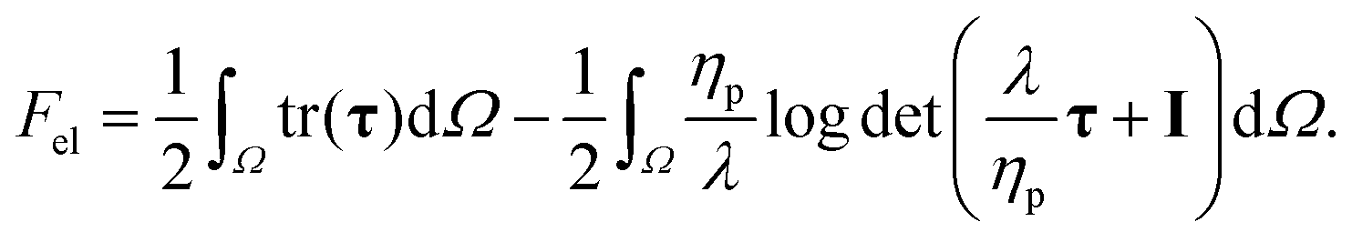 | (8) |
The model parameters of the Giesekus model (see Table 1) are calculated by fitting the predictions of the model in simple shear and small amplitude oscillatory shear using the experimental data discussed already in Section 2.1.1 and is shown in Fig. 2. Fielding and coworkers gave a simple and efficient rule for choosing the stress diffusion Ds in numerical simulations:82,94 . This rule is based on the interface width between the shear bands that scales as
  . With respect to our experiments, with a channel width of W = 8 × 10⁻⁴ m and a relaxation time of λ = 1.54 s, we find a value of Ds ≈ 4 × 10⁻¹¹ m2 s−1. For numerical stability, we relax this value to Ds = 4 × 10⁻¹⁰ m2 s−1. This stress diffusion coefficient lies within the range of experimental measurements for similar WLM solutions58,95–102 and thus we expect the difference to Fielding and coworkers’ rule to be negligible. Moreover, we note that in the simulations the corresponding interface width, assuming the flow is fully shear-banded, corresponds to ≈0.04W, which is discussed further in the ESI,† Section S1. For short (L ≪ W) and shallow (D ≪ W) geometries the interface width is expected to influence the flow.99 The experimental value, see again Section S1 (ESI†), appears to be around 0.07W, though this estimate is affected by numerous sources of noise. Nevertheless, we in fact see that, although increased for numerical stability, the larger stress diffusion is potentially more appropriate for our experimental fluid. We note that the interface width appears to be relatively large compared to the channel width. Therefore, the shear-banding nature of the fluid in our geometry is not entirely established and as such we will typically refer to shear localization, referring to the region of high shear between low shear regions or near the wall, rather than shear bands.
| η p [Pa s] | η s [Pa s] | λ [s] | α | D s [m2 s−1] |
|---|---|---|---|---|
| 27.5 | 2.75 × 10⁻³ | 1.54 | 0.85 | 4 × 10⁻¹⁰ |
|
|
|
λ* | α* |
|
|---|---|---|---|---|
| 1–10−4 | 10−4 | Wi | 0.85 | 10−3 |

The eqn (3)–(5) are solved in their non-dimensional form using as scaling quantities the characteristic mean velocity U, characteristic channel width W, the zero-shear viscosity η0 = ηp + ηs, and the flow time scale W/U (see Fig. 1 and Table 1).
2.3 Simulations
The coupled non-linear eqn (3)–(5), restricted to two dimensions, are solved using the Petrov–Galerkin stabilized finite element method for viscoelastic flows (PEGAFEM-V) developed by Varchanis et al.27,103,104 Linear basis functions are used together with the Newton-Raphson method to solve the system of non-linear equations. In total, we have 6 unknown quantities at each node of the numerical mesh (Fig. 3), corresponding to the pressure p, the velocity u, and the symmetric stress tensor τ. We use steady-state simulations to explore Wi ranging from 0.1 to 30 but separately verify steadiness using a time-dependent simulation with 2nd-order backward finite differences and a time-step Δt = 0.01 at fixed Wi values starting from a zero initial state. In particular, we only probe a limited set of Wi values and assume that once a flow becomes unsteady, it will not return to steady flow for higher Wi values. This is motivated by our experimental observations. When the time-dependent simulation converge to a steady-state, they appear identical to the steady-state simulations when the two are compared. We note that according to Moorcroft and Fielding,82 we generally expect discrepancies relating to time dependence for the Giesekus model. In general, we expect only a qualitative, not quantitative, agreement with respect to experiments. | ||
| Fig. 3 Schematic of the mesh around the upstream re-entrant corner illustrating the different densities of the elements (D = W, L = W). Shown is a coarse mesh created only for visualization purposes and not for simulations. The total number of elements is 6144 compared to the actual mesh used with 393216 elements. | ||
We employ the usual no-slip and no-penetration boundary conditions (i.e., u = 0) on all walls. Furthermore, we enforce no-flux through the walls for the stress (i.e., n·∇τ = 0).58,105 At the inlet, we impose fully developed velocity and stress fields, while we apply the open boundary condition (OBC)106 at the outlet. In all simulations we use structured meshes composed of linear triangular elements. The mesh density is higher near the walls and within the cavity, where the largest elements have a maximum size of 10−2W. Near the walls, the elements have a width in wall-direction of ≲2 × 10⁻³W to account for shear localization. This value is consistent with the experimental interface width, which is of the order 10−2W. A schematic of the mesh around the expansion re-entrant corner is shown in Fig. 3 for a square cavity. The actual mesh used for the geometry has 64 times more elements. The total number of elements ranges between approximately 400000 and 4000000, accounting for the different concavity sizes. In the ESI,† Section S2 we consider the effect of mesh size on 〈u2〉 and Eel for the cavity with D = W and L = W. The accuracy of the numerical solution decreases with increasing Wi due to shear localization occurring within the bulk, acting as a primary limiting factor for the simulations. This happens because sharp variations in the deformation rate occur within the region of shear localization. We further expect a nearly singular point at the re-entrant corner.107 Due to this, we repeat our simulations with a mesh where the re-entrant corners are smoothed using a quarter circle with radius 2 × 10⁻²W, but no significant change is observed for the flow structures inside the concavity, as discussed in the ESI,† Section S3.
In some cases, the simulation fails to converge, potentially due to issues related to the interface width and/or the mesh resolution. Alternatively, the simulations may also fail due to subcritical behaviors that the first order continuation, corresponding to an equal spacing in Wi, cannot resolve. To handle such cases, we use the pseudo-arclength continuation108,109 for advancing in Wi. In this method, an auxiliary problem is solved for the solution vector T, which consists of all unknown quantities at each node including the current Wi value. The solution vector follows a trajectory in the solution space which is parameterized by the pseudo-arclength s. At step n + 1 with step size Δs, the solution vector is updated by solving the auxiliary equation:
| Ṫn·(Tn+1 − Tn) = Δs, | (9) |
3 Results and discussion
For validation purposes, we begin our presentation of the results with a brief comparison between simulation and experiment. Subsequently, we consider the mean squared velocity and elastic Helmholtz free energy derived from the numerical simulations as a function of Wi. Next, we present the bulk of our detailed numerical simulations, beginning with expansion–contraction flows and proceeding by decreasing the length L relative to the depth D until we reach cavity flows. Finally, we summarize our results and provide phase diagrams in D and L at fixed Wi.3.1 Comparison to experiment
For the comparison between experimental and simulated data, we focus on the expansion phase in the expansion–contraction regime. In Fig. 4(a) and (b) we show the velocity magnitude u and streamlines for the microchannel with D = W and L = 5W at Wi = 1 and Wi = 5. A good qualitative match is found with their corresponding simulations, shown in Fig. 4(c) and (d), respectively. In particular, in both the experiment and the simulation at Wi = 5 (Fig. 4(b) and (d)), we note the formation of lip and corner vortices at the re-entrant and salient corners upstream and downstream of the expansion plane, respectively. For the experiment at Wi = 5 a quantitatively better match in terms of vortex sizes is obtained for a higher Wi = 30 in the simulation, see Fig. 4(e). This again demonstrates that the diffusive Giesekus model only captures the flow qualitatively and some quantitative deviations are expected. Nevertheless, we note that all flow structures as well as their Wi dependence are captured by the simulations. | ||
| Fig. 4 Velocity magnitude u and streamlines in the expansion phase for the expansion–contraction D = W and L = 5W at Wi = 1 and Wi = 5 obtained from (a) and (b) the time-averaged experimental μ-PIV data and (c)–(e) the steady-state simulation. A better match with the experiment at Wi = 5 is obtained by the steady-state simulation of Wi = 30, see (e). The velocities are normalized using the flow rate and all spatial dimensions are normalized with the channel width W. In (b), (d), and (e), we note the lip vortex at the upstream re-entrant corner and the corner vortex in the downstream salient corner. | ||
A detailed discussion on the lip vortex is provided in the ESI,† Section S4, with a quantitative comparison for the lip vortex sizes between experiment and simulation in Section S4.1 (ESI†). In the next section we consider the mean squared velocity and Helmholtz free energy to provide a big picture on the fluid behavior in terms of Wi.
3.2 Mean squared velocity and elastic Helmholtz free energy
To provide a general idea about the fluid behavior, we look at the mean squared velocity over the simulation domain Ω and the elastic Helmholtz free energy of the system in relation to Wi. Overall, these results are similar to those of the straight channel, which is shown in Fig. 5(a). The mean squared velocity exhibits a progressive decrease, with a notable inflection point around Wi ≈ 0.15. The value reaches its minimum approximately at Wi ≈ 17 for the straight channel, before exhibiting a gradual resurgence. However, this minimum is notably variable across different expansion–contraction and cavity configurations. The initial decrease in the mean squared velocity is expected and due to the flattening of the flow profile within the channel, where for the straight channel the theoretical lower limit is 〈u2〉 > U2.‡ In contrast, the increase is surprising as it suggests a change, albeit small, in the high shear region near the walls at very large Wi, at least for steady-state flow. This is potentially linked to the end of the shear-banding regime in Fig. 2(a), where the local shear rate at the wall is high and the stress at the wall increases with shear rate beyond the stress plateau. | ||
| Fig. 5 Mean squared velocity 〈u2〉/U2 and elastic Helmholtz free energy Fel compared to Wi for (a) a straight channel with a total length 31W as well as concavities of various lengths L, (b) an expansion–contraction with length L = 3W showing a potentially supercritical behavior, and (c) an expansion–contraction with length L = 2.5W showing a subcritical behavior. All concavities have a depth D = W. | ||
The elastic Helmholtz free energy linearly increases with Wi until reaching a maximum at Wi ≈ 0.21 and then decays as  over the remaining range of considered Wi values. The maximum appears to coincide with the onset of shear-thinning before any shear bands are expected to form, see Fig. 2(a) and note Wi ≈ λ for the onset. After the onset of shear-thinning and when the shear localizes, stretching of the micelles is expected to take place only in the regions of high shear rate close to the walls. Meanwhile, the micelles in the plug flow within the bulk, which corresponds to a low shear band, should exhibit minimal, if any stretching.110–113 As the flow rate increases, the high shear rate regions near the walls become narrower and the elastic Helmholtz free energy decreases, explaining the maximum in the elastic Helmholtz free energy.
The channels with concavities mostly follow the behavior described above for a straight channel. However, in a few cases corresponding to shorter contraction–expansions, deviations from such behaviour are observed. In some cases, for example, we observe a sudden small drop in the mean squared velocity indicating a potentially supercritical behavior, such as shown in the insert to Fig. 5(b). In other cases, we observe multiple values in energy at moderate to large fixed Wi, with an example displayed in Fig. 5(c). While some of these are clear artifacts from the numerical method and mesh, others are qualitatively retained even upon mesh refinement. Nevertheless, as mentioned before, it is not entirely clear if these are numerical artifacts or real. To fully establish this, higher resolution simulations are likely required. We discuss this further in the ESI,† Section S5, specifically for the channel D = W and L = 2.5W shown in Fig. 5(c).
3.3 Flow structures
We now describe the flow structures as we change the length L and depth D from an expansion–contraction (L > D + W) to a cavity flow (L < D + W). This includes intermediate “transitional” flow regimes that we describe as “short expansion–contractions” (L ≳ D + W) as well as “long cavities” (L ≲ D + W). The data shown in this section uses the steady state simulation with first order continuation in Wi, with separate simulations for verifying steadiness. As stated previously, we focus on the structure inside the cavity or between the expansion and contraction planes. | ||
| Fig. 6 (a) and (b) Velocity magnitude u with streamlines and (c) and (d) flow-type parameter ξ for the expansion–contraction with depth D = W and length L = 8W at a Weissenberg number (a) and (c) Wi = 0.1 and (b) and (d) Wi = 10. The displayed data is obtained from the steady-state numerical simulations. We note that in (a) the expansion and contraction phases are independent, as shown by (c) the flow-type parameter displaying pure shear flow (ξ = 0) between expansion and contraction phases, while in (b) they interact (d) with both rotational (ξ = −1) and extensional (ξ = 1) flow being present. | ||
Before taking a closer look at the corner or lip vortices, however, we first consider the interaction between the expansion and contraction phases. Both Fig. 6(a) and (b) appear to consists of properly separated expansion and contraction phases based on the velocity magnitude and streamlines (i.e., the flow appears to become fully-developed in the region between the expansion and contraction planes). However, while this is true for the former, it is not the case for latter. To see this, we use the flow-type parameter ξ,114–116§ defined as:
 | (10) |
is the deformation rate tensor, W is the rotation rate tensor, given by the skew-symmetric part of the velocity gradient, and ‖·‖ denotes the Frobenius norm. The flow-type parameter ξ is useful to distinguish between pure rotational (ξ = −1), shear (ξ = 0), and extensional (ξ = 1) flows. In a straight channel we expect only shear flow, which similarly occurs if the expansion and contraction phases do not interact. This is typically the case at low Wi, shown in Fig. 6(c), while at higher Wi values the expansion and contraction phases interact, see Fig. 6(d). This interaction is also expected to affect the corner vortex sizes.
A closer look at the corner vortices shows that the corner vortex at the expansion decreases in size as the Weissenberg number Wi increases, after a brief span of Wi ≲ 1 where its size changes little for depths D ≥ W, displayed in Fig. 7(a) and (c). Note that the size here is measured along the length L of the expansion–contraction by extrapolating a zero stream-wise velocity to the wall. At large Wi values the upstream corner vortex starts to slowly grow again. To provoke a better data collapse, though not perfect, Fig. 7(c) uses a different definition of the Weissenberg number: since the corner vortices are inside the concavity, we should expect them to relate to the depth D. We thus define WiD = λU/D. This follows in part the results for the 4-1 contraction channel, where the corner vortex is better described when scaled using the upstream height.8 In contrast to the depth D, the length L should not play a significant role because the expansion and contraction phases separate further as this parameter is increased. With the modified Weissenberg number WiD the expansion corner vortex starts to decrease around WiD ≈ 2 for D ≥ W, as shown in Fig. 7(c). The breakdown for D = 0.5W is attributed to the stress diffusion with the interface width becoming sizeable in comparison to the other length scales,99 causing the corner vortex to smear out. Furthermore, the measured vortex size is generally smaller than its largest extent due to a “bulge” structure where streamlines above the vortex curve back near the wall, previously described by Sato et al.34
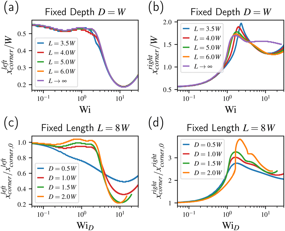 | ||
| Fig. 7 Corner vortex sizes measured along the concavity length for (a) the left corner at fixed depth D = W, (b) the right corner at fixed depth D = W, (c) the left corner normalized with the Newtonian size at fixed length L = 8W, and (d) the right corner normalized with the Newtonian size at fixed length L = 8W. The data shown is based on the steady-state numerical simulations. The Weissenberg number WiD uses the depth D as characteristic length in place of to the channel width W in eqn (1). Note that for (a) and (b) WiD = Wi. | ||
The size of the corner vortex at the contraction phase sharply increases with increasing Wi (or WiD), see Fig. 7(b) and (d), before shrinking after attaining a maximum and then, together with the other corner vortex, growing yet again but at a slower rate. The maximum occurs at around WiD ≈ 2, similar to the decrease in the expansion corner vortex. The initial increase followed by a decrease has been previously reported by Hooshyar and Germann73 in the 4-1 contraction channel for a shear-banding fluid, who attributed the increase to shear-thinning and the decrease to shear-banding. The eventual increase of the corner vortex, however, appears to relate to an interaction with the expansion phase, as we observe instead a saturation and further decrease in size with a solitary contraction. This is in contrast to the growth of the corner vortex at the expansion, which is also exhibited even without a contraction phase.
We further remark on lip vortices attached to the vertical walls at the re-entrant corners of the expansion–contraction geometries, as shown in Fig. 8, where we emphasize the expanded scaling of the x-axis due to the extreme narrowness of the vortices in the x-direction. In some cases (as in Fig. 8) such vertical lip vortices were observed at both the expansion and contraction planes, and in other cases at the expansion plane only. However, such a lip vortex at only the contraction plane was never observed. This may be explained by the relatively large size of the corner vortex at the contraction plane which engulfs any lip vortices that potentially form. Indeed, with increasing Wi, a lip vortex fixed at the contraction plane (e.g., Fig. 8(b)) is consumed by the growing corner vortex, thus forming a single vortex covering the entire corner such as in Fig. 6(b). For non-shear-thinning fluids, numerical studies typically predict the opposite and this lip vortex grows while the corner vortex decreases in size.9,10,23 The corner vortex at the expansion plane shrinks with increasing Wi and the re-entrant corner is expected to promote the formation of at least one lip vortex. This is in relation to the Pakdel–McKinley criterion,31,117 which predicts elastic instabilities due to strong curvature of streamlines and high first normal stress difference along them. The lip vortex decreases the curvature and typically forms upstream, discussed in the ESI,† Section S4, rather than downstream of the expansion re-entrant corner. A similar observation was reported by Wojcik et al.118 for a sharp bend where non-Newtonian flows typically form a lip vortex upstream, corresponding to “elasticity driven” lip vortices. Similar lip vortices have been reported by Poole et al.2,3 for expansion flows, who proposed their explanation via the Pakdel–McKinley criterion. The vertical lip vortex at the expansion plane detaches from the re-entrant corner with increasing Wi and moves to merge with the corner vortex. We emphasize that these vertical lip vortices only appear if the depth D is large enough compared to the channel width W. This is in line with numerical work on contraction channels by Alves et al.8 for a shear-thinning fluid.
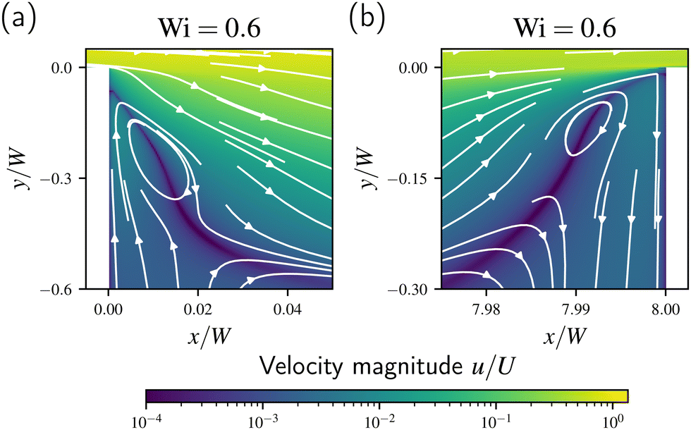 | ||
| Fig. 8 Velocity magnitude u (using a log10-scale) and streamlines for the expansion–contraction with D = W and L = 8W at Wi = 0.5 focused on (a) the vertical lip vortex at the wall of the expansion phase and (b) the vertical lip vortex at the wall of the contraction phase. These lip vortices are narrow and we emphasize the different scaling in x- and y-axis. | ||
Finally, we also point out that the expansion–contraction flows exhibit ternary vortices, Moffatt-like vortices119 that we will describe in more detail for cavity flows, and that the flows further show time dependence starting around Wi ≳ 4. Time-dependence is, however, only observed if the depth D ≥ 1.5W. We recall that time dependence is generally inadequately captured by the Giesekus model82 which may offer an explanation for this rather restricted observation on time-dependent flows.
 | ||
| Fig. 9 Velocity magnitude u and streamlines for the short expansion–contractions using the steady-state numerical data with (a) depth D = 0.5W and length L = 2W; (b) and (c) depth D = 1.5W and length L = 3W at two different Weissenberg numbers. We note the shear localization in (a) which does not align with the the boundaries of the vortices, and the extra recirculation inside the concavity in (b) compared to (c). | ||
The transitional regime proves to be numerically challenging. Alongside the deeper expansion–contraction flows, it is in particular for the short expansion–contraction at higher Wi that the pseudo-arclength continuation is required but, as mentioned before, likely does not yield accurate results. This may be due to a frustrated energy landscape, which makes the constrained minimization problem underlying the finite element method difficult to solve. It may, however, also be due to the mesh resolution and shear localization in the bulk where the elements are larger compared to the walls and the top of the concavity. These numerical issues are again discussed in the ESI,† Section S5, where we focus specifically on the short expansion–contraction.
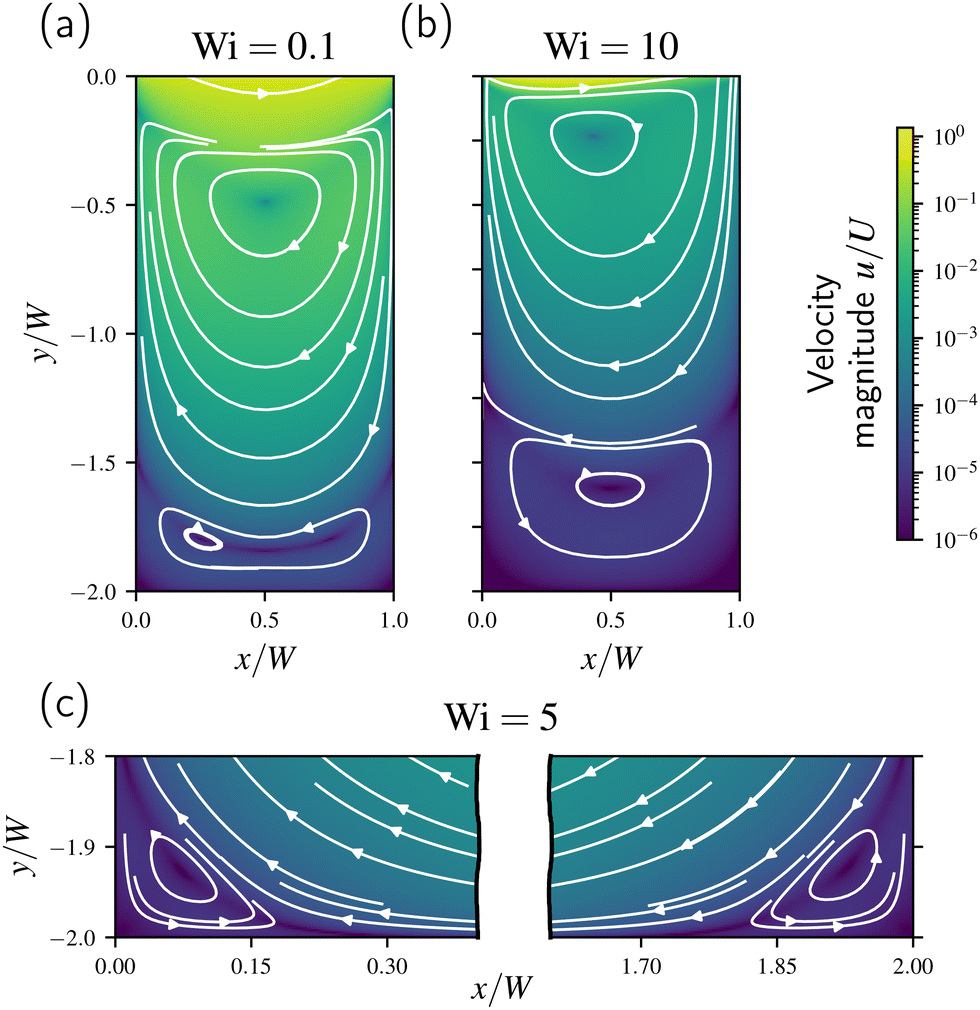
Decreasing the concavity length further leads to what we term a “long cavity”, illustrated in Fig. 10 where we only focus on the cavity section. Similar to the short expansion–contraction, the long cavity behaves as an expansion–contraction for low Wi values, Fig. 10(a), but for higher Wi transitions to a cavity with a single recirculation zone containing two vortices side-by-side, such as in Fig. 10(b). Upon further increasing Wi a single vortex forms, see Fig. 10(c). In the short expansion–contraction the distance of the shear localization from the bottom wall of the concavity decreases as Wi increases and thus expansion–contraction flow re-appears at high Wi. In contrast, for the long cavity the shear localization continuously recedes from the wall as Wi increases and the flow structures remain resembling those expected of cavity flow. Finally, as shown in Fig. 10(d) for even higher Wi the vortex splits again into two as the shear localization creates a sizeable cavity.
 | ||
| Fig. 10 Velocity magnitude u (using a log10-scale) and streamlines for a long cavity, where D = W and L = 2W, using the steady-state numerical data at (a) Wi = 0.1, (b) Wi = 1, (c) Wi = 10, and (d) Wi = 20. We note the the change from (a) an expansion–contraction towards (c) and (d) a cavity with different number of vortices. | ||
We expect both the short expansion–contraction and the long cavity to be affected by the shear localization, such as from shear-thinning or shear-banding. For example, as we have seen in the prior section and as argued by Hooshyar and Germann73 for the 4-1 contraction, the decrease in the corner vortex at the contraction plane is related to shear-banding. This likely has an effect on the short expansion–contraction and the absence of such a decrease may prevent the short expansion–contraction from recovering an expansion–contraction flow. On the other hand, for a fluid that is neither shear-thinning nor shear-banding it is often observed that this corner vortex decreases in size9,10,23 which in turn may prevent a long cavity from forming. However, further investigations using different constitutive models are required in order to make a definite statement.
 | ||
| Fig. 11 Steady-state velocity magnitude u (using log10-scale) and streamlines for the cavities (a) and (b) with length L = W and depth D = 2W or (c) with length L = 2W and depth D = 2W, at different Wi. We note the two vortices at the bottom in (a) compared to the single vortex in (b). Furthermore, the cavity and channel are separated by a region of localized shear reminiscent of a lid-driven cavity, specifically as Wi is increased. For the square cavity (c) we note the ternary vortex structures that form at the salient corners of the cavity. | ||
Overall, the cavity flow appears to approach a lid-driven cavity flow with increasing Wi, with the primary flow barely penetrating into the cavity. In this context, we can connect our observations to prior studies for lid-driven cavities. For example, given the low local Wi within the cavity due to the slow flow, we connect the split vortices at the bottom to the Newtonian case: they arise and merge from vortices located at the bottom corners as the depth D increases,24,29 see Fig. 11(c). These are again the Moffatt vortices119 mentioned in prior sections. Furthermore, as the Wi value increases the shear localization at the top of the cavity moves upwards resulting in a larger effective depth D and better approximation to the lid-driven cavity that also allows the corner vortices to merge, as shown in Fig. 11(a) and (b). The same process permits a change in the number of vortices, for example from a single vortex to two vortices stacked with the bottom split that occurs for the channel D = 2.5W and L = 1.5W (see also Fig. S9 in the ESI†). With respect to viscoelastic lid-driven flows, we emphasize the upstream shift of the upper vortex center from Fig. 11(a) and (b), which is due to the generation of large normal stresses as viscoelasticity increases.33
The analogy to the lid-driven cavity is not perfect but can be verified by fixing the aspect ratio D/L for different lengths L. This is shown in Fig. 12 for D/L = 2, where we use the flow-type parameter ξ introduced in Section 3.3.1 to show details masked by the direct velocity field. We have corrected the Weissenberg number by the geometric factor W/L, yielding what is considered a Deborah number De = λU/L for the lid-driven cavity.32,59 This is to account for the different velocities when scaling the channel dimensions. In particular, the scaling ensures that a fluid particle in the primary flow above the cavity, which drives the flow inside, takes an equal amount of time to travel the cavity length L. We highlight the clear differences in Fig. 12(a) and (d) compared to the latter two pairs. This presumably relates to the stress diffusion and the interface width,99 similar to the corner vortex at the expansion phase discussed for expansion–contraction flows. This in turn changes the shape of the driving velocity, or regularization,33 for the lid-driven cavity. Therefore, we cannot completely decouple the flow inside the cavity from the main channel when D or L are small.
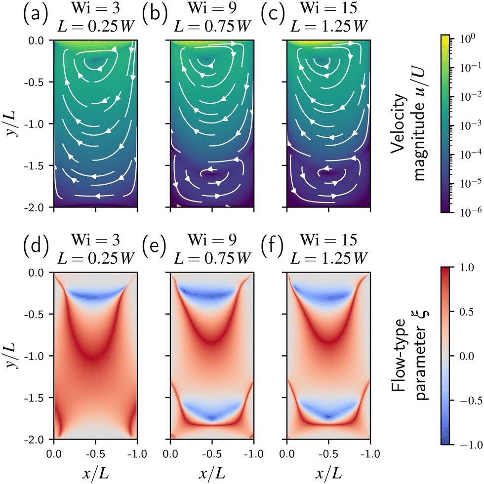 | ||
| Fig. 12 Cavities of fixed ratio D/L = 2. Displayed are (a)–(c) the steady-state velocity (using a log10-scale) with streamlines and (d)–(f) the flow-type parameter ξ. The length varies from (a) and (d) L = 0.25W, to (b) and (e) L = 0.75W, and finally (c) and (f) L = 1.25W. We adjust the Weissenberg numbers such that the Deborah number De = Wi·W/L = 12 remains constant. | ||
3.4 Flow summary: phase diagrams
We summarize the observations of the prior sections as phase diagrams in L–D at different Wi in Fig. 13, alongside some representative examples of corresponding flow states. We use again the first order continuation with the steady-state simulation. However, we have supplemented the data with simulations using the pseudo-arclength continuation where the first order continuation fails. These are marked using an overlay with diagonal lines at a 135° angle. Additionally, we indicate the onset of time-dependence (diagonal lines at a 45° angle) based on separate unsteady simulations. Several flow structures are differentiated, ranging from different types of deep cavities to expansion–contraction flows. A complete classification can be found in the ESI,† Section S6. | ||
| Fig. 13 Different flows observed based on depth D and length L at Wi = 0.2, Wi = 1, Wi = 5, and Wi = 25 using the simulation data. The different color indicate the different flow structures, ignoring finer details such as additional lip vortices in expansion–contractions. We highlight (a) and (g) deep cavities, (b) and (e) square cavities, (d) a long cavity, (f) a short expansion–contraction, and (c) and (h) expansion–contractions. The dashed line indicates the transition L = D + W. We further mark the cases where time-dependence was observed (45°-diagonals) and where the pseudo-arclength continuation was required (135°-diagonals). | ||
Overall, we differentiate two clearly distinct categories: cavity flows (blue shadings), characterized by recirculation zones spanning the length L, and expansion–contraction flows (red shading), characterized by separate corner vortices in the salient corners. These are separated by a more ambiguous transitional regime (white shading), which exhibits characteristics of both. Generally, we find that expansion–contraction flows occur when the length L exceeds the sum of the depth D and channel width W, i.e., L > D + W. On the other hand, the flow is typically a cavity flow for L ≲ D + W. This includes long cavities, which contain two vortices side-by-side within a single encapsulating recirculation zone. We emphasize that the exact flow structures in terms of number of vortices or their size depend on the Wi value. We further emphasize that the transition applies to the lengths L and depths D considered within this study. This will clearly break down as D or L are further decreased. In fact, this is already apparent in our discussion on the corner vortex sizes in the expansion–contraction flows, see Fig. 7(c), and in the discussion on the applicability of the lid-driven cavity analogy for the cavity, see Fig. 12. In both cases, we attribute these deviations to the interface width that becomes significant in size compared to the other (geometric) length scales and thus cannot be ignored. On the other hand, we also expect a breakdown simply based on geometric consideration. For example, a very shallow (D ≪ W) channel but with a comparable length and channel width L ≈ W is unlikely to sustain a cavity flow even if L < D + W. Nevertheless, the inclusion of the channel width W in the classification appears useful in the geometries we have considered and allows the inclusion of long cavities while excluding short expansion–contractions.
4 Conclusions
In this study, we have investigated the creeping flow of a fluid that exhibits strong shear localization through a geometry with a concavity on one wall. We employ two-dimensional numerical simulations, which were validated against experimental measurements of the flow at the expansion phase of the concavity. By changing the depth D and length L, different flow regimes were identified: cavity flow (L ≲ D + W), expansion–contraction flow (L > D + W), and a complex transitional regime separating the former two. Our work connects to many prior studies, which typically focus on a single aspect of our geometry or use non-shear-banding fluids. However, the concavities investigated in our study are not symmetric about the channel centreline, as is typically the case for studies on expansions and/or contractions. We also note a lip vortex upstream of the cavity or expansion plane at the re-entrant corner, which was similarly found in other studies2,3 and whose discussion can be found in the ESI,† Section S4. We simply note here that this lip vortex qualitatively differs in behavior from the structures inside the concavity, specifically in the limit of large depths D and lengths L. In this limit, the lip vortex appears to be independent of the ratio D/L and the flow inside the concavity. In contrast, the flow structures inside are expected to entirely depend on the ratio D/L.While we have examined different depths and lengths for the concavity, future studies looking at concavities at greater depths would be beneficial to validate the trends we have identified. Currently, we are limited by the computational cost associated with the large meshes required by their geometries, but the use of adaptive meshes or different programming methodologies to extend parallelization can potentially overcome this issue. The Giesekus constitutive model also provides no insights into the breaking and reformation that wormlike micelles exhibit. The use of a constitutive model including these effects, such as Vasquez–Cook–McKinley model,81 would provide additional information on the microstructural behavior of WLM solutions. Furthermore, we have focused on shear-banding fluids but fluids with other rheological properties could also yield important insights.
Finally, while numerical simulations provide an efficient method to explore various geometries and flow conditions, experimental investigations should not be neglected. Specifically conducting thorough experimental analyses in the transitional regime would greatly enhance our understanding and offer valuable insights for future research.
Author contributions
F. H.: conceptualization, data curation, formal analysis, investigation, methodology, software (minor), visualization, writing – original draft; S. V.: methodology (sim.), software, resources (sim.), supervision (sim.), writing – review & editing; C. C. H.: conceptualization (exp.), investigation (exp.), methodology (exp.), resources (exp.), supervision (exp.), writing – review & editing; S. J. H.: conceptualization (exp.), writing – review & editing; A. Q. S.: conceptualization (exp.), resources, writing – review & editing.Data availability
The data supporting this article are available within the article and the ESI.†Conflicts of interest
There are no conflicts to declare.Acknowledgements
We gratefully acknowledge the support of the Okinawa Institute of Science and Technology Graduate University (OIST) and the Scientific Computing and Data Analysis (SCDA) section of the Core Facilities at OIST. The latter provided the supercomputer Deigo, which has been used to process the experimental data and run the simulations. A. Q. S. and S. J. H. gratefully acknowledge funding support from the Japan Society for the Promotion of Science (JSPS, Grant No. 24K00810 and 24K07332, respectively). F. H. thanks Kazumi Toda-Peters for helping design and create the channels and Dr Daniel W. Carlson and Dr Ricardo Arturo López de la Cruz for insightful discussions. Finally, all authors like to extend their gratitude to the referees for their insightful comments and recommendations that have helped improve this manuscript.References
- F. T. Pinho, P. J. Oliveira and J. P. Miranda, Int. J. Heat Fluid Flow, 2003, 24, 747–761 CrossRef.
- R. J. Poole, M. A. Alves, P. J. Oliveira and F. T. Pinho, J. Non-Newtonian Fluid Mech., 2007, 146, 79–91 CrossRef CAS.
- R. J. Poole, F. T. Pinho, M. A. Alves and P. J. Oliveira, J. Non-Newtonian Fluid Mech., 2009, 163, 35–44 CrossRef CAS.
- K. Chiba, S. Tanaka and K. Nakamura, J. Non-Newtonian Fluid Mech., 1992, 42, 315–322 CrossRef CAS.
- B. Yesilata, A. Öztekin and S. Neti, J. Non-Newtonian Fluid Mech., 1999, 85, 35–62 CrossRef CAS.
- F. Olsson, J. Non-Newtonian Fluid Mech., 1994, 51, 309–340 CrossRef CAS.
- A. Baloch, P. Townsend and M. F. Webster, J. Non-Newtonian Fluid Mech., 1996, 65, 133–149 CrossRef CAS.
- M. A. Alves, P. J. Oliveira and F. T. Pinho, J. Non-Newtonian Fluid Mech., 2004, 122, 117–130 CrossRef CAS.
- F. Pimenta and M. Alves, J. Non-Newtonian Fluid Mech., 2017, 239, 85–104 CrossRef CAS.
- M. Niethammer, H. Marschall and D. Bothe, Chem. Ing. Tech., 2019, 91, 522–528 CrossRef CAS.
- J. P. Rothstein and G. H. McKinley, J. Non-Newtonian Fluid Mech., 1999, 86, 61–88 CrossRef CAS.
- J. P. Rothstein and G. H. McKinley, J. Non-Newtonian Fluid Mech., 2001, 98, 33–63 CrossRef CAS.
- L. E. Rodd, T. P. Scott, D. V. Boger, J. J. Cooper-White and G. H. McKinley, J. Non-Newtonian Fluid Mech., 2005, 129, 1–22 CrossRef CAS.
- F. Khalkhal and S. Muller, Phys. Rev. Fluids, 2022, 7, 023303 CrossRef.
- P. P. Jagdale, D. Li, X. Shao, J. B. Bostwick and X. Xuan, Micromachines, 2020, 11, 278 CrossRef PubMed.
- M. K. Raihan, S. Wu, Y. Song and X. Xuan, Soft Matter, 2021, 17, 9198–9209 RSC.
- T. Cochrane, K. Walters, M. F. Webster and W. J. G. Beynon, Philos. Trans. R. Soc. London, Ser. A, 1981, 301, 163–181 CrossRef.
- J.-H. Kim, A. Öztekin and S. Neti, J. Non-Newtonian Fluid Mech., 2000, 90, 261–281 CrossRef CAS.
- M. K. Raihan, P. P. Jagdale, S. Wu, X. Shao, J. B. Bostwick, X. Pan and X. Xuan, Micromachines, 2021, 12, 836 CrossRef PubMed.
- C.-D. Xue, Z.-Y. Zheng, G.-S. Zheng, D.-W. Zhao and K.-R. Qin, Soft Matter, 2022, 18, 3867–3877 RSC.
- X.-Y. Xu, Z.-Y. Zheng, K. Tian, D. Wang, K.-R. Qin and C.-D. Xue, Phys. Fluids, 2024, 36, 042001 CrossRef CAS.
- G. Yin, Y. Nakamura, H. Suzuki, F. Lequeux and R. Hidema, Phys. Fluids, 2024, 36, 043114 CrossRef CAS.
- M. Alves, P. Oliveira and F. Pinho, Annu. Rev. Fluid Mech., 2021, 53, 509–541 CrossRef.
- P. N. Shankar, J. Fluid Mech., 1993, 250, 371–383 CrossRef CAS.
- R. Fattal and R. Kupferman, J. Non-Newtonian Fluid Mech., 2004, 123, 281–285 CrossRef CAS.
- R. Fattal and R. Kupferman, J. Non-Newtonian Fluid Mech., 2005, 126, 23–37 CrossRef CAS.
- S. Varchanis, A. Syrakos, Y. Dimakopoulos and J. Tsamopoulos, J. Non-Newtonian Fluid Mech., 2019, 267, 78–97 CrossRef CAS.
- U. Ghia, K. N. Ghia and C. T. Shin, J. Comput. Phys., 1982, 48, 387–411 CrossRef.
- P. N. Shankar and M. D. Deshpande, Annu. Rev. Fluid Mech., 2000, 32, 93–136 CrossRef.
- H. C. Kuhlmann and F. Romanò, in The Lid-Driven Cavity, ed. A. Gelfgat, Springer International Publishing, Cham, 2019, pp. 233–309 Search PubMed.
- P. Pakdel and G. H. McKinley, Phys. Rev. Lett., 1996, 77, 2459–2462 CrossRef CAS PubMed.
- P. Pakdel, S. H. Spiegelberg and G. H. McKinley, Phys. Fluids, 1997, 9, 3123–3140 CrossRef CAS.
- R. Sousa, R. Poole, A. Afonso, F. Pinho, P. Oliveira, A. Morozov and M. Alves, J. Non-Newtonian Fluid Mech., 2016, 234, 129–138 CrossRef CAS.
- H. Sato, M. Kawata, R. Hidema and H. Suzuki, J. Non-Newtonian Fluid Mech., 2022, 310, 104946 CrossRef CAS.
- M. Pavlidis, G. Karapetsas, Y. Dimakopoulos and J. Tsamopoulos, J. Non-Newtonian Fluid Mech., 2016, 234, 201–214 CrossRef CAS.
- A. Marousis, D. Pettas, G. Karapetsas, Y. Dimakopoulos and J. Tsamopoulos, J. Fluid Mech., 2021, 915, A98 CrossRef CAS.
- M. E. Cates, Macromolecules, 1987, 20, 2289–2296 CrossRef CAS.
- J. D. Peterson and M. E. Cates, J. Rheol., 2020, 64, 1465–1496 CrossRef CAS.
- J. D. Peterson and M. E. Cates, J. Rheol., 2021, 65, 633–662 CrossRef CAS.
- J. D. Peterson and L. Gary Leal, J. Rheol., 2021, 65, 959–982 CrossRef CAS.
- J. P. Rothstein, Rheol. Rev., 2008, 2008, 1–46 Search PubMed.
- J. P. Rothstein and H. Mohammadigoushki, J. Non-Newtonian Fluid Mech., 2020, 285, 104382 CrossRef CAS.
- A. Sambasivam, A. V. Sangwai and R. Sureshkumar, Phys. Rev. Lett., 2015, 114, 158302 CrossRef PubMed.
- S. Dhakal and R. Sureshkumar, ACS Macro Lett., 2016, 5, 108–111 CrossRef CAS.
- R. Omidvar, A. Dalili, A. Mir and H. Mohammadigoushki, J. Non-Newtonian Fluid Mech., 2018, 252, 48–56 CrossRef CAS.
- A. A. Dey, Y. Modarres-Sadeghi and J. P. Rothstein, Phys. Rev. Fluids, 2018, 3, 063301 CrossRef.
- C. C. Hopkins, S. J. Haward and A. Q. Shen, Small, 2020, 16, 1903872 CrossRef CAS PubMed.
- A. A. Dey, Y. Modarres-Sadeghi, A. Lindner and J. P. Rothstein, Soft Matter, 2020, 16, 1227–1235 RSC.
- A. A. Dey, Y. Modarres-Sadeghi and J. P. Rothstein, J. Fluids Struct., 2020, 96, 103025 CrossRef.
- P. Nghe, S. M. Fielding, P. Tabeling and A. Ajdari, Phys. Rev. Lett., 2010, 104, 248303 CrossRef CAS PubMed.
- S. J. Haward, F. J. Galindo-Rosales, P. Ballesta and M. A. Alves, Appl. Phys. Lett., 2014, 104, 124101 CrossRef.
- P. F. Salipante, C. A. E. Little and S. D. Hudson, Phys. Rev. Fluids, 2017, 2, 033302 CrossRef PubMed.
- J. Yang, Curr. Opin. Colloid Interface Sci., 2002, 7, 276–281 CrossRef CAS.
- S. Ezrahi, E. Tuval and A. Aserin, Adv. Colloid Interface Sci., 2006, 128–130, 77–102 CrossRef CAS PubMed.
- C. A. Dreiss, Soft Matter, 2007, 3, 956–970 RSC.
- S. Honarmand, M. Mehraei, Z. A. Radmoghadam, E. Mohammadi, M. Dastjerdi, S. Akbari and A. Akbari, Nanosci. Technol., 2023, 10, 1–32 Search PubMed.
- T. Divoux, M. A. Fardin, S. Manneville and S. Lerouge, Annu. Rev. Fluid Mech., 2016, 48, 81–103 CrossRef.
- S. Lerouge and P. D. Olmsted, Front. Phys., 2020, 7, 246 CrossRef.
- R. J. Poole, Rheol. Bull., 2012, 53, 32–39 Search PubMed.
- J. L. White, J. Appl. Polym. Sci., 1964, 8, 2339–2357 CrossRef CAS.
- Y. Zhao, P. Cheung and A. Q. Shen, Adv. Colloid Interface Sci., 2014, 211, 34–46 CrossRef CAS PubMed.
- J. A. Pathak and S. D. Hudson, Macromolecules, 2006, 39, 8782–8792 CrossRef CAS.
- S. J. Haward, T. J. Ober, M. S. Oliveira, M. A. Alves and G. H. McKinley, Soft Matter, 2012, 8, 536–555 RSC.
- N. Dubash, P. Cheung and A. Q. Shen, Soft Matter, 2012, 8, 5847–5856 RSC.
- M. Y. Hwang, H. Mohammadigoushki and S. J. Muller, Phys. Rev. Fluids, 2017, 2, 043303 CrossRef.
- Y. Zhang, H. Mohammadigoushki, M. Y. Hwang and S. J. Muller, Phys. Rev. Fluids, 2018, 3, 093301 CrossRef.
- T. Hashimoto, K. Kido, S. Kaki, T. Yamamoto and N. Mori, Rheol. Acta, 2006, 45, 841–852 CrossRef CAS.
- V. Lutz-Bueno, J. Kohlbrecher and P. Fischer, J. Non-Newtonian Fluid Mech., 2015, 215, 8–18 CrossRef CAS.
- R. M. Matos, M. A. Alves and F. T. Pinho, Exp. Fluids, 2019, 60, 145 CrossRef.
- E. Jafari Nodoushan, Y. J. Lee, G.-H. Lee and N. Kim, Phys. Fluids, 2021, 33, 093112 CrossRef CAS.
- J. López-Aguilar, M. Webster, H. Tamaddon-Jahromi and O. Manero, J. Non-Newtonian Fluid Mech., 2014, 204, 7–21 CrossRef.
- H. Tamaddon Jahromi, M. Webster, J. Aguayo and O. Manero, J. Non-Newtonian Fluid Mech., 2011, 166, 102–117 CrossRef CAS.
- S. Hooshyar and N. Germann, Polymers, 2019, 11, 417 CrossRef PubMed.
- M. R. Stukan, E. S. Boek, J. T. Padding, W. J. Briels and J. P. Crawshaw, Soft Matter, 2008, 4, 870–879 RSC.
- M. R. Stukan, E. S. Boek, J. T. Padding and J. P. Crawshaw, Eur. Phys. J. E: Soft Matter Biol. Phys., 2008, 26, 63–71 CrossRef CAS PubMed.
- C. Sasmal, Phys. Fluids, 2020, 32, 013103 CrossRef CAS.
- R. Larson and P. S. Desai, Annu. Rev. Fluid Mech., 2015, 47, 47–65 CrossRef.
- S. Varchanis, S. J. Haward, C. C. Hopkins, J. Tsamopoulos and A. Q. Shen, J. Non-Newtonian Fluid Mech., 2022, 307, 104855 CrossRef CAS.
- H. Giesekus, J. Non-Newtonian Fluid Mech., 1982, 11, 69–109 CrossRef CAS.
- M. Johnson and D. Segalman, J. Non-Newtonian Fluid Mech., 1977, 2, 255–270 CrossRef.
- P. A. Vasquez, G. H. McKinley and L. Pamela Cook, J. Non-Newtonian Fluid Mech., 2007, 144, 122–139 CrossRef CAS.
- R. L. Moorcroft and S. M. Fielding, J. Rheol., 2014, 58, 103–147 CrossRef CAS.
- H. Rehage and H. Hoffmann, J. Phys. Chem., 1988, 92, 4712–4719 CrossRef CAS.
- H. Rehage and H. Hoffmann, Mol. Phys., 1991, 74, 933–973 CrossRef CAS.
- C. C. Hopkins, S. J. Haward and A. Q. Shen, Soft Matter, 2022, 18, 4868–4880 RSC.
- N. Burshtein, S. T. Chan, K. Toda-Peters, A. Q. Shen and S. J. Haward, Curr. Opin. Colloid Interface Sci., 2019, 43, 1–14 CrossRef CAS.
- A. Liberzon, T. Käufer, A. Bauer, P. Vennemann and E. Zimmer, OpenPIV/openpiv-python: OpenPIV-Python v0.23.4, Zenodo, 2021 DOI:10.5281/zenodo.4409178.
- A. W. El-Kareh and L. Gary Leal, J. Non-Newtonian Fluid Mech., 1989, 33, 257–287 CrossRef CAS.
- C.-Y. D. Lu, P. D. Olmsted and R. C. Ball, Phys. Rev. Lett., 2000, 84, 642–645 CrossRef CAS PubMed.
- J. H. Snoeijer, A. Pandey, M. A. Herrada and J. Eggers, Proc. R. Soc. A, 2020, 476, 20200419 CrossRef CAS PubMed.
- A. N. Beris and B. J. Edwards, Thermodynamics of Flowing Systems: with Internal Microstructure, Oxford University Press, 1994 Search PubMed.
- W. Kuhn, Kolloid-Z., 1934, 68, 2–15 CrossRef CAS.
- G. Sarti and G. Marrucci, Chem. Eng. Sci., 1973, 28, 1053–1059 CrossRef CAS.
- S. M. Fielding and P. D. Olmsted, Eur. Phys. J. E: Soft Matter Biol. Phys., 2003, 11, 65–83 CrossRef CAS PubMed.
- O. Radulescu, P. D. Olmsted, J. P. Decruppe, S. Lerouge, J.-F. Berret and G. Porte, Europhys. Lett., 2003, 62, 230 CrossRef CAS.
- P. Ballesta, M. P. Lettinga and S. Manneville, J. Rheol., 2007, 51, 1047–1072 CrossRef CAS.
- C. Masselon, J.-B. Salmon and A. Colin, Phys. Rev. Lett., 2008, 100, 038301 CrossRef PubMed.
- M. E. Helgeson, P. A. Vasquez, E. W. Kaler and N. J. Wagner, J. Rheol., 2009, 53, 727–756 CrossRef CAS.
- C. Masselon, A. Colin and P. D. Olmsted, Phys. Rev. E: Stat., Nonlinear, Soft Matter Phys., 2010, 81, 021502 CrossRef PubMed.
- M.-A. Fardin, O. Radulescu, A. Morozov, O. Cardoso, J. Browaeys and S. Lerouge, J. Rheol., 2015, 59, 1335–1362 CrossRef CAS.
- H. Mohammadigoushki and S. J. Muller, Soft Matter, 2016, 12, 1051–1061 RSC.
- P. Cheng, M. C. Burroughs, L. Gary Leal and M. E. Helgeson, Rheol. Acta, 2017, 56, 1007–1032 CrossRef CAS.
- S. Varchanis, A. Syrakos, Y. Dimakopoulos and J. Tsamopoulos, J. Non-Newtonian Fluid Mech., 2020, 284, 104365 CrossRef CAS.
- S. Varchanis and J. Tsamopoulos, Sci. Talks, 2022, 3, 100053 CrossRef.
- J. Adams, S. Fielding and P. Olmsted, J. Non-Newtonian Fluid Mech., 2008, 151, 101–118 CrossRef CAS.
- T. C. Papanastasiou, N. Malamataris and K. Ellwood, Int. J. Numer. Methods Fluids, 1992, 14, 587–608 CrossRef CAS.
- E. J. Hinch, J. Non-Newtonian Fluid Mech., 1993, 50, 161–171 CrossRef CAS.
- E. J. Doedel, V. A. Romanov, R. C. Paffenroth, H. B. Keller, D. J. Dichmann, J. Galán-Vioque and A. Vanderbauwhede, Int. J. Bifurcation Chaos, 2007, 17, 2625–2677 CrossRef.
- S. Varchanis, Y. Dimakopoulos and J. Tsamopoulos, Phys. Rev. Fluids, 2017, 2, 124001 CrossRef.
- J.-F. Berret, in Rheology of Wormlike Micelles: Equilibrium Properties and Shear Banding Transitions, ed. R. G. Weiss and P. Terech, Springer, Netherlands, Dordrecht, 2006, pp. 667–720 Search PubMed.
- Y. T. Hu and A. Lips, J. Rheol., 2005, 49, 1001–1027 CrossRef CAS.
- E. Miller and J. P. Rothstein, J. Non-Newtonian Fluid Mech., 2007, 143, 22–37 CrossRef CAS.
- J.-B. Salmon, A. Colin, S. Manneville and F. Molino, Phys. Rev. Lett., 2003, 90, 228303 CrossRef PubMed.
- P. D. Patil, J. J. Feng and S. G. Hatzikiriakos, J. Non-Newtonian Fluid Mech., 2006, 139, 44–53 CrossRef CAS.
- H. Giesekus, Rheol. Acta, 1962, 2, 101–112 CrossRef CAS.
- R. J. Poole, J. Non-Newtonian Fluid Mech., 2023, 320, 105106 CrossRef CAS.
- G. H. McKinley, P. Pakdel and A. Öztekin, J. Non-Newtonian Fluid Mech., 1996, 67, 19–47 CrossRef CAS.
- B. Wojcik, J. LaRuez, M. Cromer and L. A. Villasmil Urdaneta, Appl. Sci., 2021, 11, 6588 CrossRef CAS.
- H. K. Moffatt, J. Fluid Mech., 1964, 18, 1–18 CrossRef.
Footnotes |
| † Electronic supplementary information (ESI) available. See DOI: https://doi.org/10.1039/d4sm00594e |
| ‡ This limit value corresponds to a completely flat flow profile with slip on the walls. We emphasize that with the no-slip boundary condition the limit cannot be reached. |
§ Patils et al.114 use the symbol ψ instead. Giesekus115 defines 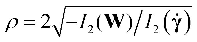 using the second invariant I2, where the flow-type parameter is recovered as ξ = (1 − ρ)/(1 + ρ). using the second invariant I2, where the flow-type parameter is recovered as ξ = (1 − ρ)/(1 + ρ). |
| This journal is © The Royal Society of Chemistry 2024 |