Shear annealing of a self-interacting sheet

Abstract

2D materials such as graphene, graphene oxide, transition metal dichalcogenides, and 2D polymers have unique properties which allow them to be used in many applications from electronics to energy to biotechnology. Producing and applying these materials often involves solution processing. Previous computational studies have observed 2D sheets in shear and extensional flows, but have focused on steady flows, even though the dynamics of these materials might exhibit hysteresis. In this work, we study 2D sheets with short-ranged attractive interactions under time-varying shear. We show that, even with relatively simple protocols, the properties of sheet suspensions can be tuned.

---

1 Introduction

2D materials, or sheets, such as graphene, graphene oxide, transition metal dichalcogenides, and, more recently, synthetic 2D polymers, have a wide breadth of applications due to their unique properties. Graphene and graphene oxide, for example, possess high surface areas, tunability (e.g. through functionalization), and favorable electrical, optical, and catalytic properties while being lightweight, flexible, and mechanically stable, allowing them to see success as membranes for separations,¹ in biomedical applications such as drug delivery,^2,3 in flexible electronic devices,⁴ and more.^5–7

In order to apply graphene and its derivatives to industrial and commercial use, it is important to be able to produce them at high quality and with relatively low cost. Many of the methods of producing graphene such as mechanical exfoliation⁸ and various bottom–up synthesis strategies,^9–11 have been restricted by high costs and/or limited scalability.^12–15 Liquid exfoliation, which typically involves using either sonication or shear of a material in solution to separate its stacked layers, represents a cheap, facile, and easily scalable method for producing 2D materials for certain applications.^15–20 Furthermore, many of the applications of graphene involve the use a suspension precursor regardless of the synthesis method (e.g. graphene inks for the printing of flexible electronics²¹). Therefore, in order to optimize the production and application of graphene as well as other 2D materials, it is important to understand how suspensions of 2D materials behave in flow.

Theoretical and computational studies have shown that the properties of sheets are greatly impacted by both their own attractive interactions^22–26 and the flow fields applied to them.^27–34 In our previous paper,³⁵ we combined these features and discovered a rich landscape of conformational properties which, when combined with the rotational behavior of the sheets, showed that the non-monotonic rheological properties and sheet orientations observed in dilute sheet suspensions^36,37 could be explained even in the athermal, dilute limit.

One question that arises when looking at our previous results is that of initial condition. Our simulations began with an initially flat sheet, but our results suggest that, for sufficiently low bending rigidities relative to interaction strength, such a state might not be accessible for a long period of time at any shear rate. Of particular importance, the no shear configuration of sheets might also look very different from a flat sheet.^38–41 It was observed that the final conformation of the sheets was highly dependent on the initial condition, leading naturally to the question of whether these sorts of conformations can be observed in real systems. More broadly, we can ask questions about how the conformations of these systems can be controlled over time by applying non-steady flows or, more generally, by varying the parameters of the system over time.

This idea is not without precedent. Suspensions of colloidal particles exhibit different microstructures, analogous to sheet conformations, depending on factors such as the shear rate and volume fraction. These microstructures, in turn, result in unique macroscopic material properties (liquids, gels, glasses, and crystals) which can be tuned for a particular application. Notably, colloidal suspensions with attractive interactions, even at volume fractions much lower than the glass transition, exhibit the same characteristic shear-thinning into shear-thickening rheological behavior seen in sheet suspensions due to the breakdown and formation of particle clusters.^42–46 The time scales for these microstructural changes cause the material to have memory of the flow history.⁴⁷ This memory allows for tuning of the final microstructure of a material through control of the applied flow protocol, for example by varying the “quenching” time from a high-shear “rejuvenation” (memoryless) regime.^48,49 Similarly, the tumbling regime for 2D sheets, which appears at high shear rates, represents a region where the conformation of sheets is continuously changing (i.e., they have access to many conformations, similar to a rejuvenation regime).^33,35 Additionally, the folded regime represents a regime where sheet conformation and rotation does not change significantly with time and where the final conformational and rotational properties of sheets possibly depends highly on the initial condition/flow history.³⁵ Thus, it makes sense to examine the 2D sheet system from a similar framework as that used for colloidal suspensions.

The remainder of the paper will be divided as follows. First, we explain our models and methods. Next, we show that the final conformation of sheets can be controlled by varying the quench time in a linear annealing simulation. Then, we implement simple step protocols utilizing the features of the phase plot discovered in previous work³⁵ to control both the conformation and orientation of sheets. Finally, we summarize our results and give our concluding remarks.

2 Models and methods

2.1 Simulation methodology

We employ the same model used in previous work³⁵, which we will describe briefly here, adapted from Silmore et al.^33,34 We generate hexagonal sheets with circumradius L = 39a, where a is the bead radius, such that each interior bead has 6 tangent neighbors, totalling N = 1141 beads. To enforce the connectivity of the sheet, we apply a harmonic potential between neighboring beads:where k is the spring constant and r₀ = 2a is the equilibrium distance between beads. We use a stiffness of k = 1000 × 6πη[small gamma, Greek, dot above]a. The continuum 2D Young's modulus, Y, which characterizes the in-plane stiffness (the “stretchiness”) of the sheet, can be connected to the discrete spring constant, k, with for this hexagonal triangulation.⁵⁰

We also apply a dihedral potential between neighboring triangles to give the sheet bending rigidity:

U_dhdl = κ(1 − n̂_i·n̂_j), (2)

where κ is the bending rigidity (out-of-plane stiffness) and n̂_i is the normal vector to triangle i. Note that these normal vectors must be consistently defined such that the potential is always positive (that is, there is always a penalty for bending). Thus, without attractive interactions, the equilibrium shape of the sheet is flat. This discrete bending rigidity can be mapped to a continuum bending rigidity, , with for this hexagonal triangulation.⁵¹

The values of k and κ were chosen such that the in-plane stiffness of sheets is much larger than their out-of-plane stiffness, as is true in many real systems. This can be quantified using the Föppl–von Kármán number, FvK ∼kL²/κ, which was always greater than 10³ for the simulations in this paper. Thus, the sheets are inextensible relative to bending.

We also apply hard-sphere interactions between non-neighboring beads with a pair-potential which places overlapping beads tangent to each other under Rotne–Prager–Yamakawa (RPY) dynamics, which we discuss later:

Finally, we apply a short-ranged interaction in the form of a truncated Lennard-Jones potential between non-neighboring beads:

where ε is the interaction strength and σ is the interaction range. We use a turn-on distance of r_on = 2a and cut-off radius of r_cut = 2.5σ. For all simulations, we set .

We integrate the system forward in time with an Euler–Maruyama integrator following the equations of motion

where L is the velocity gradient tensor, (L)_mn = [small gamma, Greek, dot above]δ_m1δ_n2, [small gamma, Greek, dot above] is the shear rate, and U_i is the sum of the applied potentials on bead i (the harmonic, dihedral, hard sphere, and Lennard-Jones potentials). To achieve long-range hydrodynamics, we use the Rotne–Prager–Yamakawa tensor for , which is given by ref. 52:where η is the fluid viscosity, r is the distance between two beads, and r̂ is the unit vector pointing from particle i to particle j. Note that, because we wish to study the behavior of a single, isolated sheet, we use the non-periodic RPY tensor here. Our boundary conditions for the system are still periodic such that the sheet will return to the simulation box if it leaves, but it will not interact hydrodynamically with its periodic images.

We previously identified two relevant dimensionless groups for this system. First, the relative strength of shear to interactions:

where is the interaction energy density of the sheet. Second, the relative strength of bending rigidity to interactions:

We note again in this paper that the pair of dimensionless groups χ⁻¹, K have a convenient physical interpretation. Varying χ⁻¹ at constant K corresponds to changing experimental conditions (i.e. shear rate) at constant material conditions, whereas varying K corresponds to changing the material conditions (e.g. sheet composition or solvent).

We generate initial conditions by generating a flat sheet in the flow-vorticity plane then rotating by a constant angle θ = 5° about the vorticity axis and a variable angle ϕ degrees about the flow axis. These angles are depicted visually in Fig. 1 we then run a shear simulation at constant χ⁻¹, K to generate an initial conformation. We then implement several protocols varying χ⁻¹, performing a constant χ⁻¹ simulation at the end of each protocol to gather statistics for sheet properties. These protocols are detailed in the following sections.

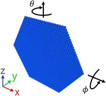Fig. 1 Depiction of initial angle conditions. θ is the angle about the vorticity (z) axis. ϕ is the angle about the flow (x) axis. y is the shear axis.

Simulations were run using HOOMD-blue on NVIDIA GeForce GTX 1080 Ti's⁵³ with a custom package from ref. 33 which was adapated from ref. 54. Averages were taken from every 100[small gamma, Greek, dot above]t due to the autocorrelation of tumbling sheets, as discussed in previous work.³⁵ All images of sheets were rendered using Ovito.⁵⁵

2.2 Sheet conformations

Here, we briefly describe and provide images of the conformational behaviors sheets can exhibit. For more detailed descriptions as well as how these sheets are classified, see previous work.³⁵ We observe four conformational behaviors for single, self-interacting sheets in shear flow: flat, tumbling, 1D folded, and 2D folded. Flat sheets are characterized by a lack of curvature throughout. Tumbling sheets are characterized by folds which are continuously changing and deforming. 1D folded sheets are characterized by parallel, persistent folds. A rolled-up sheet has either one fold along the length of the sheet or two close, parallel folds along the length of the sheet. 2D folded sheets are characterized by many, persistent folds which are not parallel. These conformations are depicted in Fig. 2, recreated from Fig. 1 in previous work.³⁵

Fig. 2 Example conformations for (a) flat, (b) tumbling, (c) 1D folded, and (d) 2D folded sheets. x is the flow direction and y is the shear direction. Recreated from previous work.³⁵

2.3 Annealing simulations

Next, we describe the time-dependent flow protocols we apply in this work. Similarly to shear protocols applied to attractive colloidal suspensions,⁴⁹ we apply a linear annealing shear protocol to sheets. First, we run a constant shear simulation at χ⁻¹ = 4.1 × 10² for 2000[small gamma, Greek, dot above]₀t, where [small gamma, Greek, dot above]₀ is the initial shear rate. Then, the shear rate is decreased linearly to zero over a variable quench time [small gamma, Greek, dot above]₀t_q, relative to the initial shear rate: [small gamma, Greek, dot above](T) = [small gamma, Greek, dot above]₀(1 − T/t_q), where T is the time since beginning the annealing process. Finally, the sheet is allowed to equilibrate at no shear for another 2000[small gamma, Greek, dot above]₀t. We choose equilibration times of 2000[small gamma, Greek, dot above]₀t to correspond to the longest time to observe conformational changes in previous work,³⁵ allowing for the collection of statistics. The largest quench time, [small gamma, Greek, dot above]₀t_q = 10 000 is chosen to be much larger than this time. The smallest quench time, [small gamma, Greek, dot above]₀t_q = 10, is chosen to be around than the typical time for a half rotation of a 1D folded sheet, which we believe to be the smallest relevant time scale for conformational changes in the system.

Averages are taken over the last 500[small gamma, Greek, dot above]₀t of the constant shear and no shear portions. We expect that, by varying the quench time, the final conformation of the sheets will vary. Specifically, as quench time increases, sheets will have more time at moderate shear rates to rearrange themselves into more energetically favorable conformations.

The equilibration period allows the interplay between interaction strength and bending rigidity to rearrange the sheet to a more energetically stable conformation. When thermal energy is larger than interaction strength, it will likely break apart folded conformations in the absence of shear.²³ However, even small thermal fluctuations may allow important rearrangements of a sheet in no shear which have important impacts on its final conformation. We do not consider such fluctuations in this work, however such a study would be valuable in the future.

We measure several properties of the final conformation: the radius of gyration, R_g, and the relative shape anisotropy, ζ². The radius of gyration is a measure of the size of a sheet. Flat sheets have the largest possible radius of gyration for an inextensible sheet (R_g ≈ 0.65L). 1D folded sheets have moderate R_g ≈ 0.5L and 2D folded sheets have smaller R_g ≲ 0.4. Tumbling sheets have widely varying values of R_g but tend to average around the value for 1D folded sheets, R_g ≈ 0.5.

The relative shape anisotropy, ζ² is a measure of the shape of a sheet. It ranges from 0 to 1, with 0 corresponding to a spherically symmetric sheet and 1 corresponding to a linear sheet. The equation for ζ² is provided in the ESI.† 1D folded sheets, who have a single large axis and are therefore “line-like,” have large values of ζ² ≈ 0.7. Flat (planar) sheets have low values of ζ² ≈ 0.25. Different 2D folded sheets can have very different values of ζ² corresponding to different fold patterns. Tumbling sheets again have widely varying values of ζ², but tend to average with very low values of ζ² ≲ 0.2, corresponding to a more “sphere-like” sheet.

These properties therefore give a more detailed description of sheets than just their conformations. Flat sheets have large R_g and low ζ², 1D folded sheets have moderate R_g and high ζ², 2D folded sheets have lower R_g and ζ² values than 1D folded sheets, and tumbling sheets typically have moderate R_g and low ζ², with larger variances in these values. The behavior of an individual sheet is dependent on the initial condition, necessitating averages over many initial conditions, given by ϕ, the initial angle about the flow axis.

2.4 Step protocols

Next, we show that the features of the phase plot can be exploited to tune the final properties of a dilute suspension of sheets. As a target, we choose 1D folded, high alignment sheets, which we would like to achieve at low shear rates. We define the alignment of a sheet as the magnitude of the dot product between the unit vector corresponding to the largest size of the sheet (v₁) with the vorticity axis (the z-axis, ẑ). Thus, the alignment varies from 0 to 1 and is a measure of the orientation of a sheet with respect to the vorticity axis (high alignments correspond to a sheet whose largest axis lies along the vorticity axis). This value was shown previously³⁵ to correspond to the viscosity of a dilute suspension of sheets, with high alignments corresponding to lower viscosities. In this work, we use the eigenvector of the gyration tensor corresponding to its largest eigenvalue as opposed to the largest semi-axis of the minimum bounding ellipsoid, as it points in a similar direction and is much cheaper to calculate.

Flat sheets have alignments which depend on their orientation. Flat sheets which rotate about the voriticity axis have alignments close to 0 while flat sheets in the flow-vorticity plane can have a range of alignments (as they have more than one largest axis). 2D folded sheets similarly have a range of alignments corresponding to the particular orbit they occupy. Tumbling sheets, on the other hand, tend to have alignments close to what would be achieved with a random sheet orientation, |v₁·ẑ| ≈ 0.52. This makes sense, as these sheets tend to have low values of ζ² and therefore little preference for different alignments in shear. 1D folded sheets tend to have alignments close to 0 or 1 depending on the initial condition, with 1 being more likely for higher shear rates.³⁵

A suspension with high alignment might have favorable macroscopic properties. For example, this suspension would have the minimal viscosity for a dilute suspension for a particular value of K as seen in previous work.³⁵ In addition, this suspension would be highly ordered and thus might carry favorable electronic properties, packing properties when concentrated, etc. We would like to achieve this state from both the high-shear tumbling regime and from folded sheets with lower alignments, which would suggest that this desired state could be achieved from many initial conditions. In particular, achieving this state from tumbling would be desirable as tumbling accesses many different configurations.

To achieve this, we note the features of Fig. 7 from previous work,³⁵ recreated in Fig. 3. In particular, this figure shows that high alignment for sheets with relatively low values of K is achieved at values of χ⁻¹ just before the tumbling transition (1.4 × 10¹ ≲ χ⁻¹ ≲ 1.4 × 10²). While these results were achieved from flat initial configurations, it is likely that these shear rates have the effect of creating 1D folded, high alignment sheets. The mechanism for changing average alignments was discussed in previous work, having to do with the deformability of these sheets allowing them to shift Jeffrey orbits.^56–58 As χ⁻¹ increases, the low alignment state becomes less favorable due to its higher stress, causing an increase in the high alignment state. However, it remains to be seen if this high alignment can be achieved from 1D folded sheets which are already in low alignment orbits. Because sheet sections can slide along each other, this region likely has the additional effect of rearranging 2D folded sheets into lower stress, more energetically favorable 1D folded sheets. At large enough values of χ⁻¹, the sheets tumble and alignment is broken down due to the low relative shape anisotropy of tumbling sheets, leading to this Goldilocks zone for alignment. Therefore, targeting this region requires knowledge of the tumbling transition for sheets.

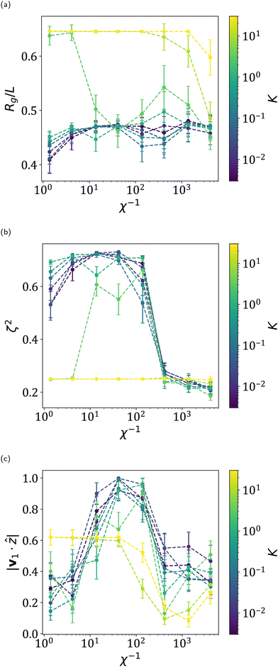Fig. 3 (a) Radius of gyration, (b) relative shape anisotropy, and (c) alignment starting from flat initial configurations and averaged over the last 200[small gamma, Greek, dot above]t of 2000[small gamma, Greek, dot above]t and all ϕ. Error bars are 95% confidence intervals. Dotted lines drawn to guide the eye. Recreated from previous work.³⁵ Note that we use a slightly different definition for the alignment here as in the rest of this work, as described in Section 2.4.

We design two step protocols to target this region. Protocol 1 starts in the 1D folded regime at moderate alignments, χ⁻¹ = 1.4 × 10¹ (Step 0), and steps into the high alignment zone, χ⁻¹ = 1.4 × 10² (Step 1), before stepping back down to the original χ⁻¹ = 1.4 × 10¹ (Step 2). Each step is run for equal strains of 2000[small gamma, Greek, dot above]t, where [small gamma, Greek, dot above] is the shear rate at each step. This protocol is run at a variety of K. We visualize this protocol on an abstraction of the phase plot from previous work,³⁵ seen in Fig. 4. The shape of this abstraction is explained in previous work.³⁵

Fig. 4 Abstractions of different annealing protocols. Shaded regions denote the steady state conformational phase map discovered in previous work.³⁵ Dots with numbers indicate constant χ⁻¹ simulations run for 2000[small gamma, Greek, dot above]t. Arrows represent a factor of 10 change in χ⁻¹. (a) Protocol 1, which starts at χ⁻¹ = 1.4 × 10¹. (b) Protocol 2, which starts at χ⁻¹ = 1.4 × 10³. The boundary between the flat/tumbling and tumbling regions lies at about K = 1. The boundary between the tumbling and 1D folded regions lies at about χ⁻¹ = 1.4 × 10². The boundary between the 1D/2D folded and 1D folded regions lies at about χ⁻¹ = 1.4. For detailed values, see Fig. 4 from previous work.³⁵

For tunability, it is important that high alignment is achieved upon increasing χ⁻¹ and is maintained upon returning to the lower χ⁻¹. Once sheets are in a high alignment state, we don't expect reducing χ⁻¹ to produce a mechanism for alignment to decrease, as the low alignment state still produces higher stresses than the high alignment state, making it likely that the high alignment state can be retained.

Protocol 2 starts in the tumbling regime, χ⁻¹ = 1.4 × 10³ (Step 0), steps into the high alignment zone, χ⁻¹ = 1.4 × 10² (Step 1), then steps down to χ⁻¹ = 1.4 × 10¹. Each step is again run for 2000[small gamma, Greek, dot above]t and this protocol is also run at a variety of K. This protocol tests if high alignment, 1D folded sheets can be generated from the tumbling regime, which accesses many more configurations than the 1D folded regime. We visualize this protocol in Fig. 4.

We calculate the radius of gyration, R_g, and relative shape anisotropy, ζ², as before, as well as the alignment, |v₁·ẑ| of these simulations. Again, the behavior of an individual sheet is erratic, necessitating averages over many initial conditions, given by ϕ, the initial angle about the flow axis.

3 Results and discussion

3.1 Annealing simulations

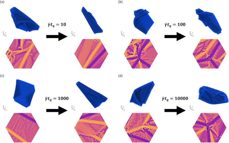
In these simulations, sheets start in the tumbling regime at varying K (χ⁻¹ = 4.1 × 10²) and are annealed to no shear over a variable quench time t_q. Sample configurations along with their corresponding signed local mean curvature (SLMC, as described in Silmore et al.³³) at the start of annealing ([small gamma, Greek, dot above]₀t = 2000) and at the end of the simulation ([small gamma, Greek, dot above]₀t = 4000 + [small gamma, Greek, dot above]₀t_q) for K = 0.03 are shown in Fig. 5. A video of an annealing simulation can be found in the ESI.† The images on the left of each subfigure, which correspond to tumbling sheets, can display a variety of folding patterns. After annealing, the sheets appear to become more compact due to the presence of attractive interactions (for K ≲ 1). However, the behavior of an individual sheet depends on its configuration at the onset of annealing. Therefore, it is necessary to look at averages over many initial conditions.

Fig. 5 Sample configurations (top) and their corresponding signed local mean curvatures (bottom), shown before (left) and after (right) annealing, for K = 0.03 and (a) [small gamma, Greek, dot above]₀t_q = 10, (b) [small gamma, Greek, dot above]₀t_q = 100, (c) [small gamma, Greek, dot above]₀t_q = 1000, and (d) [small gamma, Greek, dot above]₀t_q = 10 000. Before annealing, sheets are sheared with a constant χ⁻¹ = 4.1 × 10², which is in the tumbling regime. In configurations, x is the flow direction and y is the shear direction. Signed local mean curvature plots are all drawn to the same scale.

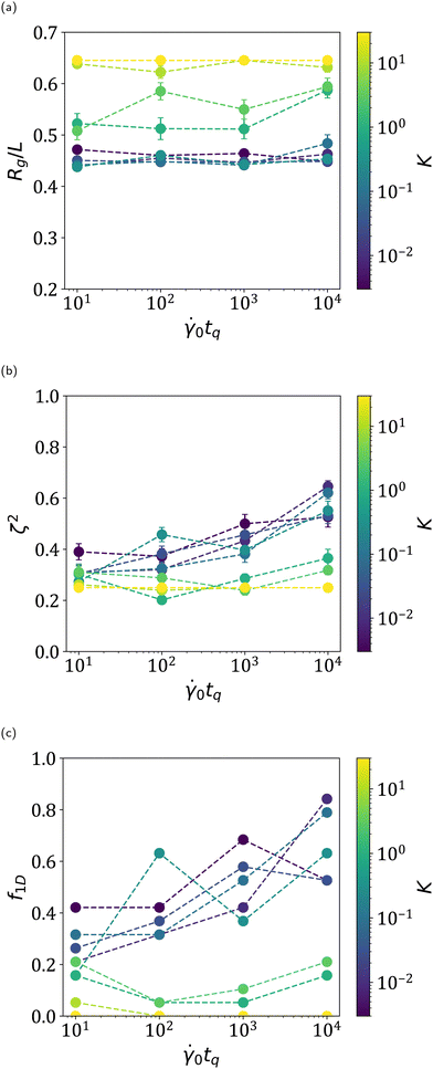
We report summary statistics for the final sheet configurations in Fig. 6. For K ≲ 1, the radius of gyration does not change much with quench time. Its approximate value of 0.45L is smaller than tumbling sheets, showing that sheets become more compact due to attractive interactions to a fairly consistent value, which makes sense for K ≲ 1, as attractive interaction can overcome bending rigidity. For K ≳ 1, there are flat sheets as well as folded sheets, causing a higher average radius of gyration.

Fig. 6 Sheet (a) radius of gyration and (b) relative shape anisotropy as a function of quench time, averaged over the last 500[small gamma, Greek, dot above]₀t of the no shear portion of annealing simulations and all ϕ. Error bars indicate 95% confidence intervals. (c) The fraction of sheets which were 1D folded after annealing. Dotted lines are drawn to guide the eye.

For K ≲ 1, the relative shape anisotropy of the sheets increases with quench time. This indicates that sheets on average exhibit more 1D folded conformations. Indeed, Fig. 6c calculates the fraction of sheets which are 1D folded, which matches with the relative shape anisotropy. This makes sense, as 1D folded sheets are slightly more energetically favorable than 2D folded sheets. Longer quench times gives more time for sheets which were more 2D folded-like to anneal towards this more energetically favorable conformation. The fraction of 1D folded sheets not increasing monotonically and instead only trending upwards is due to two reasons. First, it is possibly a sampling error due to the relatively few number of initial conditions sampled (19). Second, because this is a classification scheme where all sheets are classified as either flat, 1D folded, or 2D folded, subtle changes in the average behavior of the sheets (such as ζ²) are not picked up on. This highlights the importance of considering these summary statistics in our analyses. For moderate K ∼ 1, the relative shape anisotropy and fraction of 1D folded sheets also increased with quench time due to increased annealing, although the trend is suppressed because most sheets were flat in this regime. We suspect the initial decrease to be due to the relatively small number of annealing strain cycles causing larger variance in the final sheet conformations. For K ≳ 10, the relative shape anisotropy is relatively constant, corresponding to nearly all sheets being flat.

These results show that controlling quench time can indeed influence the final conformations of sheets. While the size of the sheets, even in the athermal limit, seems to depend on the material properties of the sheet (i.e. low or high K), the average relative shape anisotropy of the sheets increases significantly with quench time. For the shortest quench times studied here, about 20% to 40% of sheets were 1D folded. For the longest quench times studied here, most sheets (about 50% to 85%) were 1D folded. It is unknown if long enough quench times would produce nearly 100% 1D folded sheets or if there is an asymptote with this shear protocol.

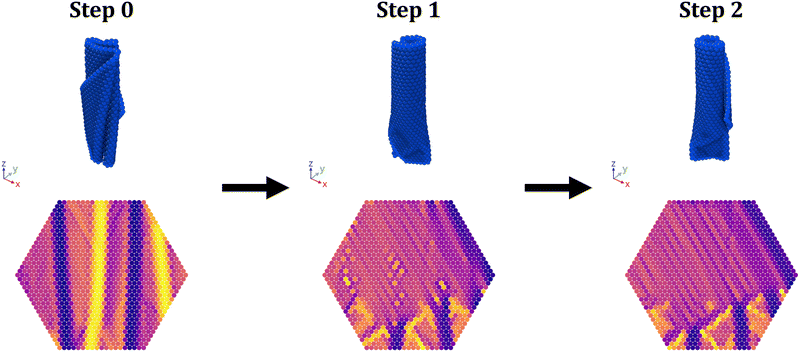
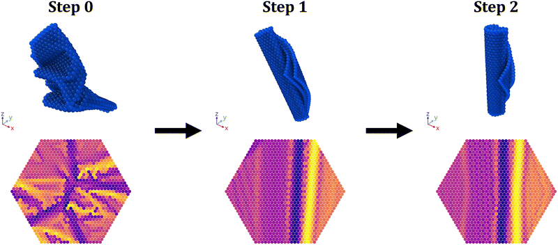
We note here that in these simulations and in the step protocol simulations, 1D folded sheets which appear at the end of protocols are usually rolled-up sheets. That is, they have either 0 or 2 folds along their center and a fairly constant curvature throughout the rest of the sheet (for example, see Step 2 in Fig. 7). These sheets have slightly larger relative shape anisotropy values than sheets with many folds as their characteristic sizes perpendicular to the largest axis tend to be closer in size. Their appearance after protocols suggests that these sheets are more kinetically accessible than sheets with many folds, as sheets with many folds require alternating curvatures, which are generated due to the initial buckling from a flat initial condition. This explains why rolled-up sheets are the more likely form of 1D folded sheet from a variety of initial conditions.

Fig. 7 Sample configurations (top) and their corresponding signed local mean curvatures (bottom), shown at the end of each constant χ⁻¹ step for Protocol 1. In configurations, x is the flow direction and y is the shear direction. Signed local mean curvature plots are all drawn to the same scale.

3.2 Step protocols

3.2.1 Protocol 1. Next, we implement step changes in χ⁻¹ to try to achieve high alignment and 1D folding. In Protocol 1, sheets are in the 1D folded regime for the whole simulation. Sample configurations at the end of each constant χ⁻¹ step are shown in Fig. 7. A sample video for a Protocol 1 simulation can be found in the ESI.†

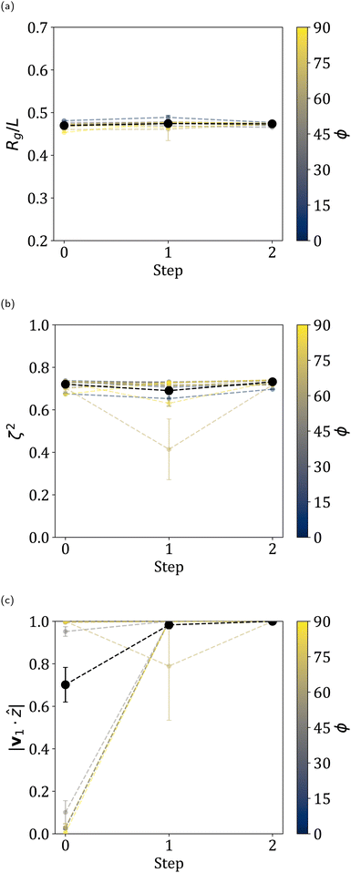
We report the summary statistics for the sheets averaged over the last 500[small gamma, Greek, dot above]t of each step in Fig. 8. These plots for all initial conditions for the example value of K = 0.03 are shown in Fig. 9 and these plots for all individual values K are provided in the ESI.† For all K, the radius of gyration and relative shape anisotropy do not change significantly, showing that most sheets remained 1D folded throughout the simulations. Furthermore, the average alignment of these sheets shows that sheets are indeed aligned upon moving to the high alignment region at Step 1. This is despite many sheets having near-zero average alignments during Step 0. This confirms that this region can induce alignment in sheets from a variety of initial conditions, even a low alignment condition. Significantly, this high alignment is maintained upon returning to the original χ⁻¹ in Step 2, as expected and desired. Even though sheets stayed 1D folded, their folds could change. In particular, higher shear rates allowed for fold annealing and the formation of rolled-up sheets, for example as seen in Fig. 7.

Fig. 8 Sheet (a) radius of gyration, (b) relative shape anisotropy, and (c) alignment averaged over the last 500[small gamma, Greek, dot above]t of each step for Protocol 1. Error bars indicate 95% confidence intervals and dotted lines are drawn to guide the eye.

Fig. 9 Sheet (a) radius of gyration, (b) relative shape anisotropy, and (c) alignment for each initial condition with K = 0.03, averaged over the last 500[small gamma, Greek, dot above]t of each step for Protocol 1. Black lines indicate the weighted average over all initial conditions. Error bars indicate 95% confidence intervals and dotted lines are drawn to guide the eye.

Note that the one sheet with K = 0.03 whose relative shape anisotropy decreased significantly in Step 1 exhibited teacup behavior, which is a classification of tumbling discussed in previous work.³⁵ This behavior involves several slowly sliding folds which continuously flip in sequence. Returning to a lower χ⁻¹ in Step 2 caused this sheet to return to a high alignment, 1D folded conformation. However, this was not always the case for sheets exhibiting teacup behavior in Step 1. Some sheets became 2D folded in Step 2, while others became low alignment, 1D folded sheets. This is why the achieved alignment for many K ≤ 1.0 was not perfect and indicates that avoiding tumbling is potentially important for achieving consistently high alignments and 1D folding, although the behavior was rare for all K.

For large enough K ≳ 3, the average radius of gyration is higher, the average relative shape anisotropy is lower, and the average alignment is lower. Examination of individual simulations reveals that this is due to the presence of a fraction of flat sheets. Some of these flat sheets become 1D folded at Step 1 due to the higher χ⁻¹, as indicated by the decrease in average radius of gyration and increase in relative shape anisotropy. Because flat sheets in the flow-vorticity plane can have a variety of alignments due to having two large axes, this makes the average alignment for large K lower, even though most sheets are either high alignment 1D folded sheets or flat sheets in the flow-vorticity plane. Together, these data show that the final properties of the suspension can indeed be changed by modifying flow protocol.

3.2.2 Protocol 2. In Protocol 2, sheets start in the tumbling regime, are moved to the high alignment region, then χ⁻¹ is lowered further. Sample configurations at the end of each constant χ⁻¹ step are shown in Fig. 10. A sample video for a Protocol 2 simulation can be found in the ESI.†

Fig. 10 Sample configurations (top) and their corresponding signed local mean curvatures (bottom), shown at the end of each constant χ⁻¹ step for Protocol 2. In configurations, x is the flow direction and y is the shear direction. Signed local mean curvature plots are all drawn to the same scale.

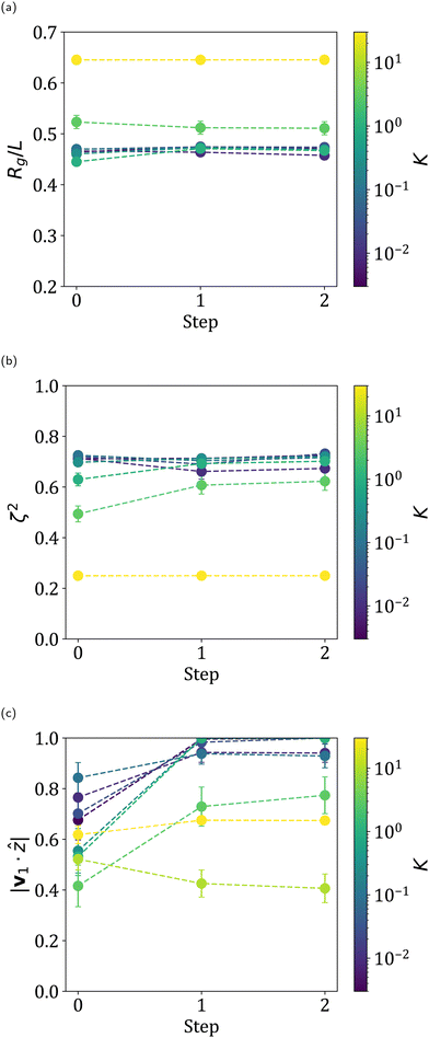
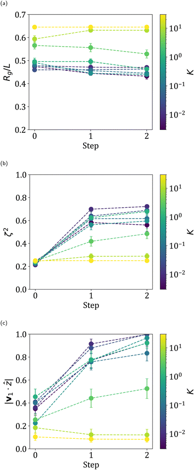
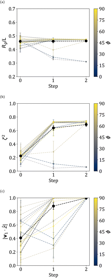
We report the summary statistics for the sheets averaged over the last 500[small gamma, Greek, dot above]t of each step in Fig. 11. These plots for all initial conditions for the example value of K = 0.03 are shown in Fig. 12 and these plots for all individual values K are provided in the ESI.† For K ≲ 1 and from Step 0 to Step 1, the radius of gyration of the sheets stays approximately the same while the relative shape anisotropy increases. This shows that sheets are indeed transitioning from tumbling to 1D folded from Step 0 to Step 1. The alignment also increases from Step 0 to Step 1, as expected, with sheets transitioning from a roughly random orientation with tumbling to high alignment 1D folded conformations. Interestingly, this increase also occurs from Step 1 to Step 2. This means that not only does entering the high alignment regime increase alignment, but changing χ⁻¹ within the folding regime also can increase the average alignment of sheets. Lower values of χ⁻¹, even outside the high alignment regime, can change the rotational behavior of sheets, evidently allowing sheets to adopt new, lower stress orbits. Notably, the final alignment decreases with increasing K, suggesting that sheet deformability is key for sheet alignment.

Fig. 11 Sheet (a) radius of gyration, (b) relative shape anisotropy, and (c) alignment averaged over the last 500[small gamma, Greek, dot above]t of each step for Protocol 2. Error bars indicate 95% confidence intervals and dotted lines are drawn to guide the eye.

Fig. 12 Sheet (a) radius of gyration, (b) relative shape anisotropy, and (c) alignment for each initial condition with K = 0.03, averaged over the last 500[small gamma, Greek, dot above]t of each step for Protocol 2. Black lines indicate the weighted average over all initial conditions. Error bars indicate 95% confidence intervals and dotted lines are drawn to guide the eye.

Analysis of individual simulations also shows several sheets adopt high average alignment 2D folded behavior, observed in Fig. 12 as low radius of gyration and relative shape anisotropy behavior, which originates from teacup tumbling behavior described and depicted in previous work.³⁵ This step change from tumbling, therefore, is highly dependent on initial condition, with the final behavior being either high alignment 1D folded or 2D folded. For K ≳ 3.0, the behavior is similar, but with the presence of flat sheets causing higher radii of gyration, lower relative shape anisotropies, and lower average alignments. For K = 30.0, every sheet is flat throughout the simulation, causing no significant change in any summary statistic.

Together, these data show that, even from the tumbling regime where sheets sample many different configurations, high alignment, 1D folded behavior can be achieved using fairly simple shear protocols.

4 Conclusions

In this work, we examine several time-dependent protocols for self-interacting, semi-flexible sheets in simple shear. Through linear annealing from tumbling to zero shear, we show that the average final properties of the sheets (in the athermal limit) can be tuned through varying the quench time. In particular, while the radius of gyration of sheets remains about the same regardless of quench time, the relative shape anisotropy increases due to the increased presence of 1D folded sheets. For large enough K, sheets are flat instead and these trends disappear.

Next, by implementing step changes in χ⁻¹, we show that sheets can also be aligned. Specifically, we show that sheets in the 1D folded regime can be aligned by increasing χ⁻¹ to a value in a high alignment regime, which lies just below the tumbling transition. This alignment is maintained upon returning to a lower value of χ⁻¹, showing hysteresis in the rotational behavior of these sheets. This protocol could be used to tune bulk properties. For example, a suspension of high alignment sheets has a lower viscosity than sheets at the same shear rate but lower average alignments. For large enough values of K, sheets are flat, and the trends disappear.

We also show that alignment can be achieved from the tumbling regime, again by stepping into the high alignment 1D folding regime before decreasing the value of χ⁻¹ lower. Interestingly, the alignment of these sheets increases upon lowering χ⁻¹ below the high alignment regime, showing that changing χ⁻¹ within the folded regime allows sheets to adopt new, lower stress orbits. The final conformations of these sheets are 1D folded or 2D folded, depending on the initial condition. The final alignment decreasing with K suggests that deformability is vital to achieving high alignment. Again, for large enough values of K, sheets are flat, and the trends disappear.

It is possible that further design is possible, for example by varying the time at each step, the values of χ⁻¹ at each step, the time between steps, or the applied rate of change of χ⁻¹ between steps, or by implementing more complex protocols with more steps. For example, due to the increase in average alignment from Step 1 to Step 2 in Protocol 2, a cyclic shear protocol which avoids the tumbling regime might achieve even better alignments after several cycles.

Furthermore, it might be possible to tune sheet properties even more specifically by introducing changes in K as well as χ⁻¹. This might be achieved experimentally, for example, by changing solvent to induce more or less favorable self-interactions and/or bending rigidities (see, for instance, work by Tang et al.^38,39) or by varying temperature to induce changes in bending rigidity.^59–62 Studies on the effect of protocols varying K would be valuable.

We note here that our simulations do not explore the entire space of potential sheet conformations. For example, kinetoplast sheets exhibit “puckered” equilibrium behavior⁶³ and nanoplatelets can be induced to have a helical structure through the addition of ligands.⁴⁰ Examination of the responses of these sorts of initial conditions to shear would be valuable, although care must be taken as these materials might exhibit inhomogeneities (e.g. kinetoplast densities at the rim versus the interior of the sheet).

Using simple protocols to traverse the χ⁻¹, K phase space, we show that the conformational and rotational properties of sheets can be tuned with varying degrees of consistency. We hope that this work can help inform the design of such protocols to produce sheets with the desired properties.

Author contributions

William T. Funkenbusch – methodology, investigation, visualization & writing. Kevin S. Silmore – methodology & writing. Patrick S. Doyle – supervision & writing.

Data availability

Sample scripts for running the simulations presented in this work can be found at https://github.com/wfunkenbusch/annealing_sample_scripts.

Conflicts of interest

There are no conflicts to declare.

Acknowledgements

Patrick S. Doyle acknowledges partial support from a Robert T. Haslam (1911) chair and NSF Grant CBET-1936696.

Notes and references

1. N. Nidamanuri, Y. Li, Q. Li and M. Dong, Eng. Sci., 2020, 9, 3–16.
2. P. Kumar, P. Huo, R. Zhang and B. Liu, Nanomaterials, 2019, 9, 737.
3. S. Goenka, V. Sant and S. Sant, J. Controlled Release, 2014, 173, 75–88.
4. R. You, Y.-Q. Liu, Y.-L. Hao, D.-D. Han, Y.-L. Zhang and Z. You, Adv. Mater., 2020, 32, 1901981.
5. J. Mu, F. Gao, G. Cui, S. Wang, S. Tang and Z. Li, Prog. Org. Coat., 2021, 157, 106321.
6. S. M. Majhi, A. Mirzaei, H. W. Kim, S. S. Kim and T. W. Kim, Nano Energy, 2021, 79, 105369.
7. B. Wang, T. Ruan, Y. Chen, F. Jin, L. Peng, Y. Zhou, D. Wang and S. Dou, Energy Storage Mater., 2020, 24, 22–51.
8. K. S. Novoselov, A. K. Geim, S. V. Morozov, D.-E. Jiang, Y. Zhang, S. V. Dubonos, I. V. Grigorieva and A. A. Firsov, Science, 2004, 306, 666–669.
9. I. Shtepliuk, V. Khranovskyy and R. Yakimova, Semicond. Sci. Technol., 2016, 31, 113004.
10. V. Agarwal and P. B. Zetterlund, Chem. Eng. J., 2021, 405, 127018.
11. F. Liu, P. Li, H. An, P. Peng, B. McLean and F. Ding, Adv. Funct. Mater., 2022, 32, 2203191.
12. R. Raccichini, A. Varzi, S. Passerini and B. Scrosati, Nat. Mater., 2015, 14, 271–279.
13. K. S. Novoselov, V. I. Fal'ko, L. Colombo, P. R. Gellert, M. G. Schwab and K. Kim, Nature, 2012, 490, 192–200.
14. S. H. Choi, S. J. Yun, Y. S. Won, C. S. Oh, S. M. Kim, K. K. Kim and Y. H. Lee, Nat. Commun., 2022, 13, 1484.
15. J. Phiri, P. Gane and T. C. Maloney, J. Mater. Sci., 2017, 52, 8321–8337.
16. U. Khan, A. O'Neill, M. Lotya, S. De and J. N. Coleman, Small, 2010, 6, 864–871.
17. J. N. Coleman, M. Lotya, A. O’Neill, S. D. Bergin, P. J. King, U. Khan, K. Young, A. Gaucher, S. De and R. J. Smith, et al. , Science, 2011, 331, 568–571.
18. Y. Hernandez, V. Nicolosi, M. Lotya, F. M. Blighe, Z. Sun, S. De, I. T. McGovern, B. Holland, M. Byrne and Y. K. Gun'Ko, et al. , Nat. Nanotechnol., 2008, 3, 563–568.
19. A. Ciesielski and P. Samor, Chem. Soc. Rev., 2014, 43, 381–398.
20. K. R. Paton, E. Varrla, C. Backes, R. J. Smith, U. Khan, A. O’Neill, C. Boland, M. Lotya, O. M. Istrate and P. King, et al. , Nat. Mater., 2014, 13, 624–630.
21. T. S. Tran, N. K. Dutta and N. R. Choudhury, Adv. Colloid Interface Sci., 2018, 261, 41–61.
22. F. F. Abraham and D. R. Nelson, J. Phys., 1990, 51, 2653–2672.
23. F. F. Abraham and M. Kardar, Science, 1991, 252, 419–422.
24. D. Liu and M. Plischke, Phys. Rev. A: At., Mol., Opt. Phys., 1992, 45, 7139.
25. G. S. Grest and I. B. Petsche, Phys. Rev. E: Stat. Phys., Plasmas, Fluids, Relat. Interdiscip. Top., 1994, 50, R1737.
26. P. Li, S. Wang, F. Meng, Y. Wang, F. Guo, S. Rajendran, C. Gao, Z. Xu and Z. Xu, Macromolecules, 2020, 53, 10421–10430.
27. Y. Xu and M. J. Green, J. Chem. Phys., 2014, 141, 024905.
28. Y. Xu and M. J. Green, J. Polym. Sci., Part B: Polym. Phys., 2015, 53, 1247–1253.
29. Y. Yu and M. D. Graham, Soft Matter, 2021, 17, 543–553.
30. Y. Yu and M. D. Graham, Phys. Rev. Fluids, 2022, 7, 023601.
31. G. Salussolia, C. Kamal, J. Stafford, N. Pugno and L. Botto, Phys. Fluids, 2022, 34, 053311.
32. H. Perrin, H. Li and L. Botto, Phys. Rev. Fluids, 2023, 8, 124103.
33. K. S. Silmore, M. S. Strano and J. W. Swan, Soft Matter, 2021, 17, 4707–4718.
34. K. S. Silmore, M. S. Strano and J. W. Swan, Soft Matter, 2022, 18, 768–782.
35. W. T. Funkenbusch, K. S. Silmore and P. S. Doyle, Soft Matter, 2024, 20, 4474–4487.
36. X. Zhang, Y. Tang, X. Wang, J. Zhang, D. Guo and X. Zhang, J. Polym. Environ., 2018, 26, 3502–3510.
37. Y. H. Shim, H. Ahn, S. Lee, S. O. Kim and S. Y. Kim, ACS Nano, 2021, 15, 13453–13462.
38. B. Tang, Z. Xiong, X. Yun and X. Wang, Nanoscale, 2018, 10, 4113–4122.
39. B. Tang, E. Gao, Z. Xiong, B. Dang, Z. Xu and X. Wang, Chem. Mater., 2018, 30, 5951–5960.
40. H. Po, C. Dabard, B. Roman, E. Reyssat, J. Bico, B. Baptiste, E. Lhuillier and S. Ithurria, ACS Nano, 2022, 16, 2901–2909.
41. D. Monego, S. Dutta, D. Grossman, M. Krapez, P. Bauer, A. Hubley, J. Margueritat, B. Mahler, A. Widmer-Cooper and B. Abécassis, Proc. Natl. Acad. Sci. U. S. A., 2024, 121, e2316299121.
42. J. F. Brady and G. Bossis, Annu. Rev. Fluid Mech., 1988, 20, 111–157.
43. G. Bossis and J. Brady, J. Chem. Phys., 1989, 91, 1866–1874.
44. J. Bender and N. J. Wagner, J. Rheol., 1996, 40, 899–916.
45. J. Bergenholtz, J. Brady and M. Vicic, J. Fluid Mech., 2002, 456, 239–275.
46. J. Mewis and N. J. Wagner, Colloidal suspension rheology, Cambridge University Press, 2012.
47. S. Jamali, G. H. McKinley and R. C. Armstrong, Phys. Rev. Lett., 2017, 118, 048003.
48. N. Koumakis, E. Moghimi, R. Besseling, W. C. Poon, J. F. Brady and G. Petekidis, Soft Matter, 2015, 11, 4640–4648.
49. S. Jamali, R. C. Armstrong and G. H. McKinley, Mater. Today Adv., 2020, 5, 100026.
50. M. J. Bowick, A. Košmrlj, D. R. Nelson and R. Sknepnek, Phys. Rev. B, 2017, 95, 104109.
51. G. Gompper and D. Kroll, J. Phys. I, 1996, 6, 1305–1320.
52. J. Rotne and S. Prager, J. Chem. Phys., 1969, 50, 4831–4837.
53. J. A. Anderson, J. Glaser and S. C. Glotzer, Comput. Mater. Sci., 2020, 173, 109363.
54. A. M. Fiore, F. Balboa Usabiaga, A. Donev and J. W. Swan, J. Chem. Phys., 2017, 146, 124116.
55. A. Stukowski, Modell. Simul. Mater. Sci. Eng., 2009, 18, 015012.
56. G. I. Taylor, Proc. R. Soc. London, Ser. A, 1923, 103, 58–61.
57. T. Omori, Y. Imai, T. Yamaguchi and T. Ishikawa, Phys. Rev. Lett., 2012, 108, 138102.
58. H. Zhao and E. S. Shaqfeh, J. Fluid Mech., 2013, 725, 709–731.
59. D. Nelson, T. Piran and S. Weinberg, Statistical mechanics of membranes and surfaces, World Scientific, 2004.
60. D. Nelson and L. Peliti, J. Phys., 1987, 48, 1085–1092.
61. P. Liu and Y. Zhang, Appl. Phys. Lett., 2009, 94, 231912.
62. A. Fasolino, J. Los and M. I. Katsnelson, Nat. Mater., 2007, 6, 858–861.
63. A. R. Klotz, B. W. Soh and P. S. Doyle, Proc. Natl. Acad. Sci. U. S. A., 2020, 117, 121–127.

---

Footnote

† Electronic supplementary information (ESI) available: Videos of different shear protocols and summary statistics for protocols 1 and 2. See DOI: https://doi.org/10.1039/d4sm00710g

---