BOTTS: broadband optimized time–temperature superposition for vastly accelerated viscoelastic data acquisition

Abstract

Modern materials design strategies take advantage of the increasing amount of materials property data available and increasingly complex algorithms to take advantage of those data. However, viscoelastic materials resist this trend towards increased data rates due to their inherent time-dependent properties. Therefore, viscoelasticity measurements present a roadblock for data collection in an important aspect of material design. For thermorheologically simple (TRS) materials, time–temperature superposition (TTS) made relaxation spectrum measurements faster relative to, for example, very long creep experiments. However, TTS itself currently faces a speed limit originating in the common logarithmic discrete frequency sweep (DFS) mode of operation. In DFS, the measurement time is proportional (by a factor much greater than one) to the lowest frequency of measurement. This state of affairs has not improved for TTS for half a century or more. We utilize recent work in experimental rheometry on windowed chirps to collect three decades of complex modulus data simultaneously, resulting in a ∼500% increase in data collection. In BOTTS, we superpose several isothermal chirp responses to produce a master curve in a fraction of time required by the traditional DFS-TTS technique. The chirp responses have good, albeit nontrivial, signal-to-noise properties. We use linear error propagation and a noise-weighted least squares approach to automatically incorporate all the data into a reliable shifting method. Using model thermoset polymers, we show that DFS-TTS and BOTTS results are comparable, and therefore BOTTS data represent a first step towards a faster method for master curve generation from unmodified rheological measurement instruments.

---

Introduction

To “Harness the Power of Materials Data” is a primary goal of the 2021 Materials Genome Initiative Strategic Plan.¹ This goal includes the application of data hungry methods to ever-larger data sets for the purpose of extracting new insights into material structure–processing–property relationships and thereby accelerating material development. However, datasets for some fundamental material properties – including viscoelastic properties – remain simultaneously (i) sparsely scattered throughout the literature and (ii) difficult and time-consuming to produce, which creates a bottleneck that hinders the wide-spread consistent archival of FAIR materials data. In this article, we provide an improved pathway towards resolving obstacle (i) and address obstacle (ii) directly.

Realistic simulations of property and performance for polymer-based materials and composites are essential for current industries^2–6 and are also poised to enable a revolution of application-oriented material design ranging from aerospace structures to energy storage materials to implant customization.^7–9 A robust and reliable library of the core time- and temperature-dependent polymer material properties is urgently needed to ensure sufficient accuracy of integrated multi-scale simulations for data driven material design.^10,11

For example, Iyer et al.¹² pursued the optimization of a nanocomposite maximizing dielectric breakdown strength while minimizing dielectric permittivity and dielectric loss using finite element simulations and Bayesian optimization via Gaussian process regression. To undertake the simulations, the frequency-dependent properties of polymers are required as one key input. Their work used only 3 polymers for the machine learning models, limited by the availability of sufficiently accurate data for both polymer and composite properties. This and similar other studies would be able to cover a much larger design space if a full suite of robust viscoelastic properties were readily available for polymers and their composites.^13,14

For the most common polymer materials, simple scalar properties such as room temperature elastic modulus, or glass transition temperature can be found in collected works^15,16 and databases,^17–19 but the vast majority of material data is found in unstructured papers and manuscripts many of which are not in machine-readable form. For many subfields, useful data may not even exist at all,²⁰ or if it does exist, it rarely contains complete and reproducible descriptions of the experimental and computational methods used to collect those properties. Time- or frequency-dependent polymer mechanical property measurement is an especially egregious example of such a subfield, as these properties are essential for engineering components in key applications such as structural aerospace components, medical implants, and energy storage.

A viscoelastic master curve, created by superposing complex modulus data collected by rheometry (for liquids) or dynamic mechanical analysis (DMA, for solids) at several temperatures,²¹ is the usual form that frequency-dependent polymer behavior is included in engineering component design. The best and most completely specified master curves we have identified in the literature^22–24 are from scientific papers focused narrowly on the process of generating master curves themselves. In the general literature, there are significant limitations on the reported viscoelastic properties for polymers and composites in (a) the limited time or frequency range of isothermal measurement and (b) the apparent drift of material properties over time due to instrumental and experimental issues, both of which are a consequence of slow data acquisition. This article addresses these shortcomings by directly tackling the time consuming, error prone, and often highly manual generation of high-quality viscoelastic property data for polymers and composites. In particular, we introduce a rapid method that can be implemented on standard laboratory instrumentation to collect the temperature-dependent complex modulus data for thermorheologically simple (TRS) materials. This work will enable the collection of an extensive set of viscoelastic data for a range of polymers and composites, which can be archived into accessible materials data resource such as MaterialsMine,¹⁷ opening the doors to other researchers to access the array of thermomechanical property data for their own design studies.

TTS and current limitations

Traditionally, time- and temperature-dependent mechanical properties of a polymeric solid are obtained using DMA which has two fundamental operating modes: (i) a temperature sweep at fixed frequency and (ii) a frequency sweep at fixed temperature.²⁵ The temperature-dependent properties are the fastest to obtain but are valid only at the specific frequency of measurement. It has long been observed that curves of the instantaneous modulus as a function of time or frequency for many polymers retain their shape as the temperature is changed, simply shifting left or right along the log time or log frequency axis. This observation forms the core principle of the time–temperature superposition (TTS) principle.

TTS is typically implemented in practice as a frequency-temperature superposition using DMA frequency sweeps (over ∼2–3 decades of frequency) that yield the storage and loss moduli over a range of fixed temperatures that span the glass transition temperature. These curves at each temperature can be superposed, for TRS materials, via shifting on the logarithmic frequency axis, to obtain shift factors, a_T, defining the “master curve” of the properties over a large frequency/time domain, spanning from rubbery to glassy behavior of the polymer (tens of decades of frequency).²⁵ Such master curves are an invaluable input for large scale design and optimization of new polymers and composites for applications with targeted design parameters. Details on TTS theory can be found in studies by Honerkamp and Weese.²² While TTS provides a powerful method to accelerate the attainment of full spectral viscoelastic response, it still remains a time consuming and manual process.

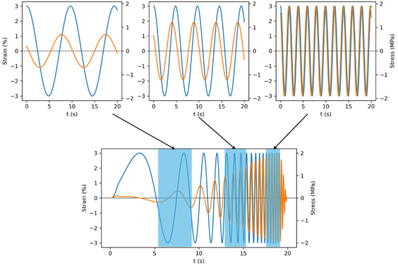
The limiting factor of master curve generation lies in the collection of the “frequency sweep” data, which in practice consists of many sequential, discrete frequency steps, with a finite residence time at each oscillation frequency (Fig. 1, top). The ensemble discrete frequency sweep (DFS) data are repeated for many specific temperatures to perform TTS (collectively, DFS-TTS). A typical mode of operation is to capture log-spaced sinusoidal data at each frequency for 1.5 cycles or 5 seconds, whichever is longer. Accordingly, a frequency sweep from 0.01 Hz to 10 Hz at 10 points per decade will take ∼17 minutes, with the lowest 3 frequencies consuming almost half the running time. In contrast with this slow data acquisition rate, the force and strain transducers sample at perhaps 500 Hz. This drastic reduction of information (500 Hz to ∼1/30 Hz on average) is the natural consequence of the traditional, single-frequency (“narrowband”) methods. However, there are some techniques that have been deployed to achieve mechanical spectroscopy at many simultaneous frequencies (“broadband”) and thereby reach the information collection potential of advanced rheometers and DMAs (Fig. 1, bottom).

Fig. 1 Synthetic stress strain response from a Maxwell material with a relaxation time of 0.5 s. Strain curves are depicted in blue and use the left y-axis. Stress curves are shown in orange and use the right y-axis (top). Sinusoidal strain response at 0.1, 0.2, and 0.5 Hz (left to right). (bottom) Exponential chirp response from 0.05 Hz to 5 Hz. Information from shaded-chirp regions approximately corresponds to the sine response indicated by arrows.

Broadband DMA techniques

Optimal Fourier Rheometry²⁶ (OFR) is a method which is broadly suitable for broadband mechanical spectroscopy, offering improvements over earlier broadband techniques that could provide comparable speedup like Fourier Transform Mechanical Spectroscopy²⁷ (FTMS or MultiWave (MW)) and I-Rheo²⁸ because it uses a broadband mechanical strain impulse (a “chirp”) with (a) a consistent maximum mechanical strain input to avoid escaping the linear regime and (b) a 1/f^α power spectrum (sometimes called a “pink” spectrum) to maintain the signal-to-noise ratio (SNR) at low frequencies.^26,29 OFR can be seen as a limiting case of MW where the amplitude and shifts of the many driving frequencies have a specific relationship. The OFR method has been used to measure the linear viscoelastic (LVE) properties of alginate during the process of gelation, minimizing interference in the measurement of the material's property changes (“mutation”) over time. Optimally Windowed Chirps²⁹ (OWChs) minimize error from both signal attenuation and spectral leakage due to abrupt strain changes at the ends of a rectangular windowed chirp, the latter being particularly relevant in the context of TTS as the periodic structure of the leakage artifact²⁹ makes it hard to identify a single best shift factor. OWCh has been deployed for the measurement of viscoelasticity during casein gelation.²⁹ OFR and OWCh represent a significant improvement in time-optimal complex modulus measurement, although demonstrated only in fluids and only for time-limited applications. However, the technique is in principle instrument and geometry independent; the only requirement is to be able to feed an arbitrary strain (or stress) profile into the strain-controlled (or stress-controlled) element of the instrument, and to read back the response in real time. To our knowledge, optimally windowed chirps have not yet been implemented with DMA for the purpose of rapidly acquiring master curves of solids by TTS. Therefore, an enormous potential exists to adapt this approach to improve and accelerate master curve generation for TRS solids.

BOTTS

In this work, we outline our new approach, broadband optimized time–temperature superposition (BOTTS), which adapts broadband excitations to fully utilize the capabilities of existing rheological measurement instruments for the rapid collection of viscoelastic material properties from macroscale solid specimens in standard DMA instrumentation. We show that our method accelerates master curve data acquisition in DMA for viscoelastic solid polymers by 500%. We demonstrate on a model material that the superposition of storage and loss moduli recorded via broadband chirps at different temperatures is achievable in theory and in practice. Using mutually consistent experimental protocols and superposition algorithms, we compare and contrast master curves and shift factors as generated by DFS-TTS and BOTTS for our model material to show that the output of both techniques is comparable, and therefore BOTTS is comparable to the existing methods while being five-fold faster.

Experimental section

Photopolymer resin PT

Oxygen-tolerant thiol–ene resins with narrow glass transitions were synthesized according to Nair.³⁰ All components were purchased from Millipore-Sigma and used as received. The thiol crosslinker, pentaerythritol tetrakis(3-mercaptopropionate) (PETMP) was mixed in a stoichiometric ratio with the allyl crosslinker 1,3,5-triallyl-1,3,5-triazine-2,4,6(1H,3H,5H)-trione (TATATO). The PETMP-TATATO (PT) resin was stabilized with 0.1% 4-methoxyphenol (MEHQ) by mass, which was mixed on a 40 °C stirrer plate until dissolved. The stabilized resin was photosensitized by mixing 1% 2-hydroxy-4′-(2-hydroxyethoxy)-2-methylpropiophenone (D2959) by mass on a 40 °C stir plate, protected from ambient light by wrapping the vial in foil, overnight or until fully dissolved.

PT resin was poured into a Sylgard 184 (Dow) silicone mold for 8 × 2 × 40 mm bar specimens and cured in air under 256 nm light for 30 minutes in an Asiga Flash curing oven and post-cured at 65 °C overnight in a Shel Lab vacuum oven to maximize photosensitizer conversion.

Epoxy resin DI

All components were purchased from Millipore-Sigma and used as received. Epoxy monomer 2,2-bis[4-(glycidyloxy)phenyl]propane (diglycidyl ether of bisphenol A, DGEBA) with epoxide equivalent weight 172–176 g mol⁻¹ was mixed in a stoichiometric ratio with 5-amino-1,3,3-trimethylcyclohexanemethylamine (isophorone diamine, IPDA) having amine hydrogen equivalent weight 42.5 g mol⁻¹ to form DGEBA–IPDA (DI) resin.

DI resin was poured into a Sylgard 184 (Dow) silicone mold for 8 × 2 × 40 mm bar specimens. The mold and resin were placed in a Shel Lab vacuum degassed for 10 minutes under a vacuum at 80 °C, then allowed to cure at ambient pressure according to the following automatic temperature profile: soak for 1 h at 80 °C, ramp to 180 °C for 1 h, soak for 2 h at 180 °C, and then end the process by disabling the heater and allowing the temperature to passively return to ambient temperature.

DMA

All dynamic mechanical analyses were performed on an RSA-G2 rheometer (TA Instruments) with a forced convection oven using the 25 mm 3-point bend geometry. Bar specimens were trimmed and shaped with 180 grit sandpaper where necessary. Autotension was used to adjust the gap to maintain a static “compression” force of 0.2 N. Strain sweeps were performed in the rubbery, glassy, and glass transition regimes of all materials to verify linear viscoelastic (LVE) behavior. Prior to any DFS or BOTTS temperature sweep, a temperature ramp was performed using the oven attachment with air, at −5 °C min⁻¹ measuring cyclic response at 1 Hz with AutoStrain maintaining an oscillation force of 0.01 N to 0.015 N across the glass transitions. This was done to reset specimens to a consistent thermal history and collect (or double check) approximately optimal strains for good signal-to-noise ratios at all temperatures of interest. Strains varied from 0.001 to 0.1.

Discrete frequency sweeps

All frequency sweeps were performed within a single “Temperature sweep” step in TRIOS software, which is a combined step that automatically holds a sequence of evenly spaced temperatures (we consistently selected 5 °C apart). Between each step, we used an isothermal, static, Autotension-active delay (pre-soak) time set to 120 seconds to allow for heat transfer to the specimen and three-point bend tooling. The pre-soak is followed by the main isothermal frequency sweep step, a sinusoidal (i.e., DFS) measurement of complex modulus across frequencies from 0.014 Hz to 14 Hz at 10 discrete frequencies per decade.

Windowed chirps

The broadband mechanical impulse (or “chirp”) is a finite time, non-sinusoidal applied strain that causes mechanical deformation at many effective frequencies simultaneously. For information on the properties of chirps and the importance of windowing functions, we refer readers to the studies by Ghiringhelli²⁶ and Geri,²⁹ respectively. The definition for the padded, inverse-Gaussian-windowed, exponential strain chirp used in the rest of this work is:where ε₀ is the requested nominal strain amplitude, t is the time from the start of the overall arbitrary wave, p is the time of the zero strain padding before and after the chirp, T is the total length of the windowed chirp steps (i.e., 2p less than the total data collection time), r is the width parameter of the Gaussian window function, ω₁ is the lowest requested frequency in radians per second, and ω₂ is the highest requested frequency in radians per second. The Tukey-windowed chirp of Geri et al.²⁹ is not used here due to technical software constraints as explained in the next section.

BOTTS implementation

These chirps are implemented in the TRIOS (TA Instruments) “Arbitrary wave” step, being careful to observe an intrinsic 80-character limit on the length of the equation string. To achieve a constant temperature during the experiment, the temperature field for each equation was set to the overall step temperature setpoint. The exact input strings are:
and should be compared to eqn (1) with the values p = 1 s, T = 210 s, r = 0.05, ω₁ = 0.03 rad s⁻¹, and ω₂ = 188.5 rad s⁻¹, which we use consistently in this work. The new “variables” x, y, and z are single digits that form a “scientific notation” encoding for ε₀ which varies by temperature and material. The sampling rate is set to 500 Hz in all cases, although the TRIOS software automatically reduces the sampling rate when the number of points per “arbitrary wave” would exceed an intrinsic limit of 32768, so we observe an effective sampling rate of 156.78 Hz. This also caps our theoretical dynamic range at 4.2 decades of frequency.

Because there is an intrinsic 4-piece limit to the piecewise function definition slots available in the TRIOS Arbitrary Wave step, the padding steps before and after the chirp require our chirp to be completely defined within the remaining two available steps. However, the 80-character limit prevents us from including multiple windowing factors in a single step leading to our two-part piecewise definition here. These limits prevent us from using the Tukey window as described by Geri et al.²⁹ as the definition of that chirp requires three of the four available steps.

Data processing and filtering

We exported data from Trios in .xls format and read it using Python packages Pandas and xlrd. DFS data needed no further processing. For BOTTS, we used the padding steps to reliably detrend the chirp response before Fourier analysis. Detrending is a common signal processing technique to suppress noise and ringing artifacts from low frequency drifts,³¹ and in this application, we used it to mitigate spurious strain drift – apparently originating in thermal drift due to finite temperature soak delay. Due to an instrumental artifact, we discard the first 0.5 s of data. The second 0.5 s and the last 0.5 s of stress and strain data are fit to determine and subtract a linear detrending function for each. The detrended data from 0.5 s to 212 s were transformed using rfft provided by NumPy.³² The ratio of the resultant complex stress and strain arrays formed the complex Young's modulus used for TTS.

We used the bounded version of Brent's method for scalar minimization³³ to optimize the shift factor between each adjacent pair of isothermal data series. For the objective function, we used the variance weighted sum of squared residuals from independent 10th order weighted polynomial fits to storage and loss moduli against log(frequency). This is comparable to the method of Honerkamp and Weese²² except we estimate shifts pairwise and do not apply the logarithmic transform to the modulus data.

We performed Prony series regressions against master curves at two relaxation modes per decade plus an extra plateau modulus mode with ElasticNetCV from scikit-learn³⁴ using parameters,

which produced Prony coefficients practically comparable to sign-controlled Tikhonov-regularized fits,^21,35,36 but with additional L₁ regularization and an interface which automatically selects the regularization hyperparameters through cross-validation.

Results and discussion

In this section, we first demonstrate, using data from two different polymers, both the traditional DFS data acquisition method for viscoelastic moduli and the new broadband BOTTS approach, highlighting the acceleration of data acquisition. This data acquisition acceleration occurs as the frequency-dependent modulus data are obtained at each independent temperature. We then review the traditional method for TTS using DFS and present how TTS is performed in the BOTTS approach, where a consistent weighting of the chirp data is utilized. Finally, we compare the data sets for the complete viscoelastic master curve products of the traditional DFS-TTS and BOTTS approaches, showing that the new accelerated method achieves high quality consistent VE modulus data.

Comparing broad- and narrowband modulus data acquisition

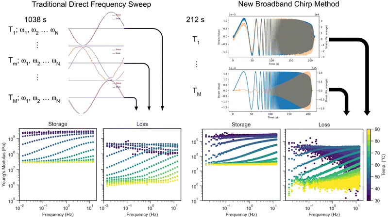
To demonstrate the relative data quality of our new chirp-based BOTTS technique to that of traditional DFS-TTS (narrowband), we compare three decades of isothermal frequency data at 5 °C intervals from 30 °C to 90 °C obtained from the traditional DFS technique and the new technique on the same PT polymer specimen (Fig. 2). The experimental settings were deliberately chosen to be as similar as possible for the DFS and BOTTS methods, including identical specimens, quench rates, temperature steps, soak times, and strain amplitudes. Since the DFS data are collected one frequency at a time, the constant temperature measurement process at each step lasts 1038 seconds. In comparison, the strain chirp induces a material response at many frequencies simultaneously, and our instrument collects three decades of frequency data in only 212 seconds, a five-fold improvement in throughput during the data collection step. As can be seen in Fig. 2, the resultant storage and loss modulus data from DFS and exponential chirps are very similar at each temperature, although they have important quantitative differences.

Fig. 2 Comparison of log-spaced direct frequency sweep (DFS) (left) and broadband chirp (right) approaches to temperature-dependent modulus measurement. While the storage and loss moduli match between approaches in terms of magnitude and frequency trend at each T_M, data density and variance differ.

The first difference is that the modulus data from the BOTTS method are linearly and much more densely sampled in frequency. While this dense sampling is an inevitable consequence of capturing more information from the experiment, it also increases computational requirements for data storage and viscoelastic analysis. It may be practical to create logarithmically spaced bins to represent average complex modulus behavior more efficiently in the case of high dynamic range chirps, but in this work, we never reach a dataset size where this step was necessary, and working with the unbinned data makes handling uncertainty more straightforward.

The second difference is the significant spread in the data for measurements at high frequency in the broadband data. While at first blush the spread in the data seems to add uncertainty, in fact we can use the dense data sampling together with a high-quality estimate of the noise variance to create a precise estimate of the true underlying complex modulus. DFS data are often treated as having a constant relative error,²⁴ and often with an arbitrary scaling factor. Broadband data are derived from a Fourier transform, so the noise floor can be estimated through the power at frequencies well above the highest requested chirp frequency ω₂. Then, a linear propagation of theoretical frequency-independent noise through the complex modulus calculation produces an estimate of the noise spectrum. The ratio of storage modulus to error is always above 10, but the ratio of loss modulus to error at high frequencies in the elastic cases can drop well below that threshold, as shown in Fig. 3.

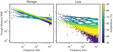Fig. 3 Complex Young's modulus magnitude over the propagated error, i.e., “Signal-to-Noise Ratio” (SNR) for chirps on PT resin at each temperature.

Consequently, scatter appears in the loss modulus while the storage modulus remains tight. Details of the data sampling and error propagation are provided in the ESI.† Despite the presence of this scatter, we will demonstrate in upcoming sections that the presence of this scatter need not interfere with the generation of master curves and shift factors.

Superposition of broadband and narrowband modulus data

The graphical superposition on a logarithmic plot of modulus data from different temperatures is essentially an assertion of the statement,where is the frequency-dependent complex modulus at temperature T and a_T and b_T are the horizontal and vertical shift factors, respectively. If the statement holds, the material is considered TRS. E* can be generally described by a sum of Maxwell elements, sometimes called a Prony series,which is valid in the linear viscoelastic (LVE) regime. Importantly, combining the shift factors with this Prony series representation showsmeaning each individual Maxwell element uniformly experiences a factor of b_T more apparent strain and a factor of a_T higher apparent frequency at T compared to the reference temperature when subjected to the same actual sinusoidal strain. TRS materials can be thought of as having a one-to-one correspondence between a molecular-scale relaxation and a Maxwell element.

In the case of the DFS technique, the application of the above is straightforward. A constant temperature is held, a sinusoidal strain is driven at each frequency ε(ω), the initial unsteady state is discarded, and the lagged sinusoidal stress is recorded, containing the sum of the influence of each Maxwell element at that frequency. The complex modulus is calculated by measuring the phase lag, δ(ω), and stress magnitude, σ(ω), to further calculate |E*| = σ/ε and converting to its real and imaginary components,

E*(ω) = |E*|cos (δ) + i|E*|sin (δ) = E′(ω) + iE′′(ω), (5)

where E′(ω) and E′′(ω) are the storage and loss moduli, respectively.²⁵ At the next temperature, this is all repeated and, for TRS materials, all the elements experience shift factors at each temperature that are frequency independent. This renders the curves for E′(ω) and E′′(ω) superposable, and the superposition of these curves via the shift factor, a_T(T), yields the master curve for the polymer at the chosen reference temperature.

In the case of broadband excitation as in BOTTS, there is an arbitrary strain function that obscures the connection of the stress function to the Prony series representation. Fortunately, we have already assumed LVE properties above, so we can rely on the property of frequency orthogonality. Therefore, taking the Fourier transform of the stress and strain, we generate a representation of all the component sines and cosines that compose our broadband impulse and response. Then, as the waves form an orthogonal basis, we can consider each of the components individually, applying the same logic as in DFS when interpreting the data and when superposing two curves. The only difference here is that we have digitally isolated the response at each frequency instead of through our choice of driving function.

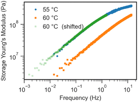
To demonstrate the practical superposition of broadband frequency response data, the storage modulus E′ of PT resin obtained by Fourier transform of a windowed chirp and its response at both 55 °C and 60 °C are displayed along with a shifted display of the 60 °C data shown in Fig. 4. The shifted modulus data overlap well over the entire two decades of frequency that the series have in common. This overlap is empirical evidence suggesting that BOTTS will work as a basis to form a master curve.

Fig. 4 Broadband storage Young's modulus of PT resin at 55 °C (blue) and 60 °C (orange) and 60 °C data shifted by a factor of 10 (green). The overlap of the green and blue data indicates a high-quality shift.

Although it is straightforward to superpose the broadband curves “by eye,” we wish to provide a consistent basis to compare the performance of the BOTTS and DFS-TTS in recovering shift factors and master curves. Therefore, we follow the method of Honerkamp and Weese²² to fairly and reproducibly shift the data. Our specific implementation optimizes only horizontal shifts pairwise between adjacent isothermal measurements by minimizing the χ² score of weighted polynomial fits of E′ and E′′ simultaneously (see Methods for details). Vertical shift factors could be obtained by first horizontally shifting E′′/E′ = tan(δ) and subsequently obtaining vertical shifts from E′′ or E′, but we typically obtained values very near 1, so we omit this step as negligible for our data. A joint optimization of horizontal and vertical shifts is possible, but global optimization of the 2D system is complex and slow²⁴ and was unnecessary to produce satisfactory results for the purposes of this work. Quantifying the joint uncertainty of BOTTS-derived horizontal and vertical shift factors will be the subject of future research.

Master curves from BOTTS and DFS-TTS

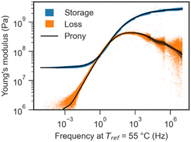
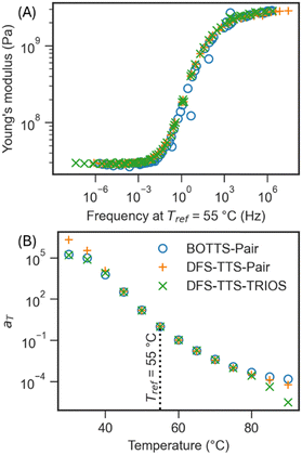
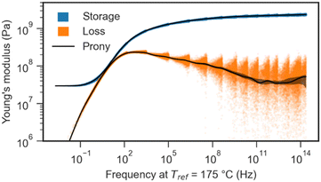
The result of performing BOTTS on PT resin data from Fig. 2 and 3 is a master curve spanning 12 orders of magnitude in frequency with a single, relatively sharp, glass transition. Heeding Winter's admonishment to check that master curves are Kramers–Kronig consistent,²¹ we overlay the BOTTS master curve with a Prony series fit shown in Fig. 5, observing good agreement between the fit and the data, supporting the physical validity of BOTTS. The large number of data points we obtain from transforming chirps means the uncertainty of the model fit is substantially smaller than the spread of the data, originating from lower SNR at high frequencies, and highly elastic (very low E′′) behavior at high temperatures.

Fig. 5 BOTTS of the PT resin data shifted horizontally using the pairwise polynomial strategy. The Prony series fit (with a bootstrapped central 90th percentile band) overlays well, showing that the resulting master curve is physically reasonable.

To compare master curves and shift factors produced from BOTTS and DFS-TTS, we collected PI viscoelastic response from both techniques over the same range of frequencies and temperatures (see Fig. 2) and subjected them to our automatic shift algorithm. As a baseline, we also generated shifts and a master curve from the same DFS data using the closed, commercial TRIOS TTS feature. The superposed storage moduli and shift factors from each are visualized together in Fig. 6.

Fig. 6 (A) Storage modulus curves and (B) horizontal shift factors for master curves from pairwise BOTTS (blue circles), pairwise DFS-TTS (orange plus), and DFS-TTS derived from the commercial TRIOS software. The reference temperature 55 °C is indicated by a dashed line.

BOTTS and DFS-TTS seem to have a similar range of validity, as the high and low frequency tails of the data in the glassy and rubbery regimes have increasing scatter between techniques with distance from the reference temperature T_ref = 55 °C. (As with any superposition, the shift factors are unity at the reference temperature.) To shift the tail regions is an intrinsically ill-posed problem, as the storage moduli plateau and the loss moduli approach the noise threshold, limiting the detectable differences between curves. Therefore, for PT resin with our experimental parameters, we would suggest only relying on shift factors in Fig. 6 from about 40 °C to 80 °C, or equivalently, moduli from 4 × 10⁻⁴ to 8 × 10⁴ Hz at T_ref.

We selected PT resin as a platform to develop BOTTS as it has a very narrow, reproducible, and stable glass transition due to its ideal network structure.³⁰ As a demonstration of the broad applicability of BOTTS, we applied the technique to DI epoxy resin without first obtaining DFS-TTS data. The DI master curve, displayed in Fig. 7, shows a broader glass transition indicative of typical heterogeneous chemical structures in epoxy thermosets.^37–39

Fig. 7 BOTTS of the PT resin data shifted horizontally using the pairwise polynomial strategy. The Prony series fit (with a bootstrapped central 90th percentile band) overlays well, showing that the resulting master curve is physically reasonable.

Beyond producing a reasonable master curve, we emphasize that the data, from 100 °C to 180 °C in 5 °C increments, were collected in just under 100 minutes, including soak time. A comparable DFS-TTS experiment would take over 500 minutes. The speedup of BOTTS provides a unique additional advantage beyond the obvious time savings: the resin spends much less time at high temperatures, avoiding thermal side reactions and property drift common in amine-epoxy and other engineering thermosets.

Conclusions

We have presented BOTTS, a DMA technique that utilizes broadband chirps to take full advantage of the data acquisition capabilities of modern DMA hardware to accelerate the collection of frequency data for time–temperature superposition by 500%. Given such an increase in data collection rate, BOTTS could enable the curation of vast quantities of high quality thermorheological data and derived master curves, shift factors, WLF parameters, and relaxation spectra. A higher instrumental bandwidth would increase the speedup to as much as 10×, and further gains could be realized in the choice of temperatures and soak times before measurement. This would decrease the cost of performing and curating data including composition, processing, and aging parameters and their uncertainties from large designs of experiments for a broad range of advanced materials. Broad uptake of this technique would lead to increased availability of reliable high-bandwidth time/frequency/temperature property data for polymers and their composites and could dramatically accelerate and increase the accuracy of design loops for new material applications. We also developed a data analysis pipeline to incorporate the unique complex modulus data output from BOTTS. Our ongoing research will seek to further improve the BOTTS strategy (including temperature steps, chirp duration, and other parameters) to minimize shift factor uncertainty given instrumental constraints and time allotment, or inversely to minimize experiment time while meeting a prescribed uncertainty of the shift factors, with direct comparison to similarly optimized MW and DFS methodologies. This optimal strategy combined with the data analysis pipeline presented in this work would unlock the possibility for a more hands-free and reproducible experience for master curve generation, eventually including fully autonomous experimentation.

Author contributions

RJS: conceptualization data curation, formal analysis, investigation, methodology, project administration, software, validation, visualization, and writing – original draft. SZ: funding acquisition, methodology, resources, supervision, and writing – review & editing. LCB: funding acquisition, methodology, resources, supervision, and writing – review and editing.

Data availability

The DMA data (TRIOS .tri and .xls formats) and code to generate the plots in this work from those DMA data or your own data generated from appropriately configured TRIOS experiments are available as ESI† and at https://github.com/richardsheridan/ChirpPy. The version of the code employed for this study was b7352ef.

Conflicts of interest

There are no conflicts to declare.

Acknowledgements

The authors would like to acknowledge funding from NSF-CMMI Award Number 2040670. The authors thank Michaela Geri and Bavand Keshavarz for helpful discussion.

Notes and references

1. NSTC Subcommittee on the Materials Genome Initiative, Materials Genome Initiative Strategic Plan, 2021.
2. A. I. Medalia, Rubber Chem. Technol., 1972, 45, 1171–1194.
3. C. Burkhart, B. Jiang, G. Papakonstantopoulos, P. Polinska, H. Xu, R. J. Sheridan, L. C. Brinson and W. Chen, Tire Sci. Technol., 2023, 51, 114–131.
4. H. Deng, Y. Liu, D. Gai, D. A. Dikin, K. W. Putz, W. Chen, L. Catherine Brinson, C. Burkhart, M. Poldneff, B. Jiang and G. J. Papakonstantopoulos, Compos. Sci. Technol., 2012, 72, 1725–1732.
5. M. Qu, F. Deng, S. M. Kalkhoran, A. Gouldstone, A. Robisson and K. J. Van Vliet, Soft Matter, 2011, 7, 1066–1077.
6. D. W. Collinson, M. D. Eaton, K. R. Shull and L. C. Brinson, Macromolecules, 2019, 52, 8940–8955.
7. National Research Council, Integrated Computational Materials Engineering: A Transformational Discipline for Improved Competitiveness and National Security, National Academies Press, Washington, D.C., 2008.
8. J. Allison, B. Cowles, J. DeLoach, T. Pollock and G. Spanos, Implementing Integrated Computational Materials Engineering (ICME) in the Aerospace, Automotive, and Maritime Industries, Miner. Met. Mater. Soc., 2013.
9. The Minerals Metals & Materials Society (TMS), Building a Materials Data Infrastructure: Opening New Pathways to Discovery and Innovation in Science and Engineering, TMS, Pittsburgh, PA, 2017.
10. B. Natarajan, Y. Li, H. Deng, L. C. Brinson and L. S. Schadler, Macromolecules, 2013, 46, 2833–2841.
11. L. C. Brinson, M. Deagen, W. Chen, J. McCusker, D. L. McGuinness, L. S. Schadler, M. Palmeri, U. Ghumman, A. Lin and B. Hu, ACS Macro Lett., 2020, 9, 1086–1094.
12. A. Iyer, Y. Zhang, A. Prasad, P. Gupta, S. Tao, Y. Wang, P. Prabhune, L. S. Schadler, L. C. Brinson and W. Chen, Mol. Syst. Des. Eng., 2020, 5, 1376–1390.
13. Y. Wang, M. Zhang, A. Lin, A. Iyer, A. S. Prasad, X. Li, Y. Zhang, L. S. Schadler, W. Chen and L. C. Brinson, Mol. Syst. Des. Eng., 2020, 5, 962–975.
14. P. Prabhune, Y. Comlek, A. Shandilya, R. Sundararaman, L. S. Schadler, L. C. Brinson and W. Chen, Nanomaterials, 2023, 13, 2394.
15. Handbook of industrial materials, Elsevier Advanced Technology, Oxford, UK, 2nd edn, 1992.
16. Polymer handbook, ed. J. Brandrup, E. H. Immergut and E. A. Grulke, Wiley, New York, Chichester, 4th edn, 2004.
17. J. P. McCusker, N. Keshan, S. Rashid, M. Deagen, C. Brinson and D. L. McGuinness, in The Semantic Web – ISWC 2020, ed. J. Z. Pan, V. Tamma, C. d’Amato, K. Janowicz, B. Fu, A. Polleres, O. Seneviratne and L. Kagal, Springer International Publishing, Cham, 2020, vol. 12507, pp. 144–159.
18. D. J. Walsh, W. Zou, L. Schneider, R. Mello, M. E. Deagen, J. Mysona, T.-S. Lin, J. J. De Pablo, K. F. Jensen, D. J. Audus and B. D. Olsen, ACS Cent. Sci., 2023, 9, 330–338.
19. S. Otsuka, I. Kuwajima, J. Hosoya, Y. Xu and M. Yamazaki, 2011 International Conference on Emerging Intelligent Data and Web Technologies, IEEE, Tirana, Albania, 2011, pp. 22–29.
20. S. M. McDonald, E. K. Augustine, Q. Lanners, C. Rudin, L. Catherine Brinson and M. L. Becker, Nat. Commun., 2023, 14, 4838.
21. H. H. Winter, J. Non-Newton. Fluid Mech., 1997, 68, 225–239.
22. J. Honerkamp and J. Weese, Rheol. Acta, 1993, 32, 57–64.
23. D. J. Plazek, J. Rheol., 1996, 40, 987–1014.
24. K. R. Lennon, G. H. McKinley and J. W. Swan, Data-Centric Eng., 2023, 4, e13.
25. H. F. Brinson and L. C. Brinson, Polymer Engineering Science and Viscoelasticity, Springer, US, Boston, MA, 2008.
26. E. Ghiringhelli, D. Roux, D. Bleses, H. Galliard and F. Caton, Rheol. Acta, 2012, 51, 413–420.
27. E. E. Holly, S. K. Venkataraman, F. Chambon and H. Henning Winter, J. Non-Newton. Fluid Mech., 1988, 27, 17–26.
28. M. Tassieri, M. Laurati, D. J. Curtis, D. W. Auhl, S. Coppola, A. Scalfati, K. Hawkins, P. R. Williams and J. M. Cooper, J. Rheol., 2016, 60, 649–660.
29. M. Geri, B. Keshavarz, T. Divoux, C. Clasen, D. J. Curtis and G. H. McKinley, Phys. Rev. X, 2018, 8, 041042.
30. D. P. Nair, PhD Thesis, University of Colorado at Boulder, 2011.
31. R. Kopel, R. Sladky, P. Laub, Y. Koush, F. Robineau, C. Hutton, N. Weiskopf, P. Vuilleumier, D. Van De Ville and F. Scharnowski, NeuroImage, 2019, 191, 421–429.
32. C. R. Harris, K. J. Millman, S. J. Van Der Walt, R. Gommers, P. Virtanen, D. Cournapeau, E. Wieser, J. Taylor, S. Berg, N. J. Smith, R. Kern, M. Picus, S. Hoyer, M. H. Van Kerkwijk, M. Brett, A. Haldane, J. F. Del Río, M. Wiebe, P. Peterson, P. Gérard-Marchant, K. Sheppard, T. Reddy, W. Weckesser, H. Abbasi, C. Gohlke and T. E. Oliphant, Nature, 2020, 585, 357–362.
33. P. Virtanen, R. Gommers, T. E. Oliphant, M. Haberland, T. Reddy, D. Cournapeau, E. Burovski, P. Peterson, W. Weckesser, J. Bright, S. J. Van Der Walt, M. Brett, J. Wilson, K. J. Millman, N. Mayorov, A. R. J. Nelson, E. Jones, R. Kern, E. Larson, C. J. Carey, İ. Polat, Y. Feng, E. W. Moore, J. VanderPlas, D. Laxalde, J. Perktold, R. Cimrman, I. Henriksen, E. A. Quintero, C. R. Harris, A. M. Archibald, A. H. Ribeiro, F. Pedregosa, P. Van Mulbregt, SciPy 1.0 Contributors, A. Vijaykumar, A. P. Bardelli, A. Rothberg, A. Hilboll, A. Kloeckner, A. Scopatz, A. Lee, A. Rokem, C. N. Woods, C. Fulton, C. Masson, C. Häggström, C. Fitzgerald, D. A. Nicholson, D. R. Hagen, D. V. Pasechnik, E. Olivetti, E. Martin, E. Wieser, F. Silva, F. Lenders, F. Wilhelm, G. Young, G. A. Price, G.-L. Ingold, G. E. Allen, G. R. Lee, H. Audren, I. Probst, J. P. Dietrich, J. Silterra, J. T. Webber, J. Slavič, J. Nothman, J. Buchner, J. Kulick, J. L. Schönberger, J. V. De Miranda Cardoso, J. Reimer, J. Harrington, J. L. C. Rodríguez, J. Nunez-Iglesias, J. Kuczynski, K. Tritz, M. Thoma, M. Newville, M. Kümmerer, M. Bolingbroke, M. Tartre, M. Pak, N. J. Smith, N. Nowaczyk, N. Shebanov, O. Pavlyk, P. A. Brodtkorb, P. Lee, R. T. McGibbon, R. Feldbauer, S. Lewis, S. Tygier, S. Sievert, S. Vigna, S. Peterson, S. More, T. Pudlik, T. Oshima, T. J. Pingel, T. P. Robitaille, T. Spura, T. R. Jones, T. Cera, T. Leslie, T. Zito, T. Krauss, U. Upadhyay, Y. O. Halchenko and Y. Vázquez-Baeza, Nat. Methods, 2020, 17, 261–272.
34. F. Pedregosa, G. Varoquaux, A. Gramfort, V. Michel, B. Thirion, O. Grisel, M. Blondel, P. Prettenhofer, R. Weiss, V. Dubourg, J. Vanderplas, A. Passos, D. Cournapeau, M. Brucher, M. Perrot and É. Duchesnay, J. Mach. Learn. Res., 2011, 12, 2825–2830.
35. J. Honerkamp and J. Weese, Rheol. Acta, 1993, 32, 65–73.
36. R. D. Bradshaw and L. C. Brinson, Mech. Time-Depend. Mater., 1997, 1, 85–108.
37. H. K. Nguyen, D. Wang, T. P. Russell and K. Nakajima, Soft Matter, 2015, 11, 1425–1433.
38. J. W. Woodcock, R. J. Sheridan, R. Beams, S. J. Stranick, W. F. Mitchell, L. C. Brinson, V. Gudapati, D. Hartman, A. Vaidya, J. W. Gilman and G. A. Holmes, Compos. Sci. Technol., 2020, 192, 108074.
39. J. W. Woodcock, S. J. Stranick, A. P. Kotula, S. H. Chen, S. Engmann, J. W. Gilman and G. A. Holmes, Polymer, 2023, 273, 125826.

---

Footnote

† Electronic supplementary information (ESI) available. See DOI: https://doi.org/10.1039/d4sm00798k

---