DOI:
10.1039/D4SM01054J
(Paper)
Soft Matter, 2024,
20, 9360-9372
Dynamics of switching processes: general results and applications in intermittent active motion
Received
3rd September 2024
, Accepted 4th November 2024
First published on 6th November 2024
Abstract
Systems switching between different dynamical phases is a ubiquitous phenomenon. The general understanding of such a process is limited. To this end, we present a general expression that captures fluctuations of a system exhibiting a switching mechanism. Specifically, we obtain an exact expression of the Laplace-transformed characteristic function of the particle's position. Then, the characteristic function is used to compute the effective diffusion coefficient of a system performing intermittent dynamics. Furthermore, we employ two examples: (1) generalized run-and-tumble active particle, and (2) an active particle switching its dynamics between generalized active run-and-tumble motion and passive Brownian motion. In each case, explicit computations of the spatial cumulants are presented. Our findings reveal that the particle's position probability density function exhibit rich behaviours due to intermittent activity. Numerical simulations confirm our findings.
1 Introduction
Switching between different dynamical phases is a widespread phenomenon in a wide range of complex systems.1–3 Many examples can be found in a biological setting, including transitions between stages of the cell-cycle,4,5 changes in animal motility patterns,6,7 diffusion of particles in mammalian cells,8,9 and target-binding proteins that switch between sliding motion along DNA strands and three-dimensional excursions.10,11
Living or active systems are ideal candidates for displaying dynamical switching.12–15 For example, such systems are often capable of processing environmental information, leading to subsequent adaptation and changes in motility patterns,16–18 a property not shared with their passive counterparts. The study of physical properties of life-like systems often falls under the umbrella of active matter.19–22 A plethora of examples can be found, ranging from motile cells23 and synthetic active colloids24 on the microscale all the way to macro-scale living organisms25 and granular systems.26–28 Several theoretical investigations of active particles that undergo dynamical switching has been seen recently, including switching chirality29–32 and particles that switch between many possible self-propulsion states.33–35 Furthermore, recent theoretical investigations show how such intermittent active phases can aid in spatial exploration and target search.17,36
A widespread type of switching found both on microscopic and macroscopic scales is activity that only acts intermittently, where directed motion is interspersed with passive or immobile phases.37–54 Interestingly, from an experimental perspective, intermittent activity can easily be achieved in systems of light-activated particles.55 Such experimental modelling of active behaviours has opened a door to design self-propelled particles with a broad range of novel behaviours,56,57 including the ability to make particles reverse their direction of motion with a specified asymmetry in the forward and backward speeds.58
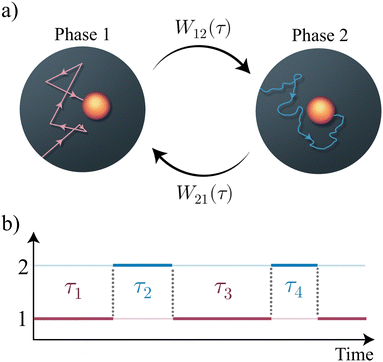
In this paper, we present a general framework that captures the dynamics of a two-phase switching process (see Fig. 1). In particular, we derive an exact expression for the (Fourier–Laplace transformed) probability density function of an observable that evolves according to the rules of two different phases. We employ the (Fourier–Laplace transformed) probability density function to compute the expression for the effective diffusion of the switching process, finding conditions on the waiting-time distribution that minimises the effective diffusivity. Motivated by the experiment based on light-activated particles,55 we study a minimal stochastic model in one-dimension involving a generalized run-and-tumble particle with intermittent passive phases. Using the results of the switching formalism, we first study the generalized run-and-tumble particle and characterise its position fluctuations, and find an optimal switching rate that maximises long-time diffusion. Then, we explore the same process with intermittent passive phases by obtaining the first few position's cumulants exactly. We also discuss the time evolution of the position distribution of the active particle with intermediate passive phases, and show interesting short- (obtained by a perturbative analysis) and long-time behaviors.
 |
| | Fig. 1 (a) Schematic representation of a two state stochastic process, where a particle iteratively switched between two arbitrary abstract dynamical phases. (b) The particle switches between phase 1 and 2 iteratively, with corresponding waiting times τ, where τ is chosen from the probability density functions W1→2(τ) ≡ W12(τ) and W2→1(τ) ≡ W21(τ). | |
The rest of the paper is organised as follows. Section 2 builds the general framework of the switching process and discusses the method to compute the fluctuations of the particle's position. Section 3 contains the derivation of the effective diffusion constant for a general scenario. In Section 4, we discuss two examples of switching processes, with detailed analysis of their time-dependent properties. Then, we discuss the position probability density function for a generalized run-and-tumble particle switching its behaviour to Brownian motion intermittently in Section 5. Finally, we summarize the paper in Section 6. Some of the detailed expressions are relegated to Appendices.
2 General formalism
In the past several decades, the theoretical statistical physics community has explored the fascinating nature of dynamical switching processes by investigating their statistical properties. Examples include modelling of dynamical coexistence of slow- and fast-diffusion in liquids and caging effects in glassy materials,59,60 as well as theoretical work on the dynamical disorder.61–63 Additionally, stochastic resetting,64–71 diffusive systems with a switching diffusion coefficient,72–76 alternating dynamical phases,77–81 and even the blinking of quantum dots82,83 fall under the umbrella of the stochastic switching process. Several frameworks have been proposed to deal with systems exhibiting dynamical switching, such as hybrid and composite stochastic processes,72,84,85 piece-wise deterministic Markov processes86 and hidden Markov models.87–89 Here, we consider a general approach to model systems with switching mechanisms, which enable us to reproduce many some of the above examples.
In this paper, we consider a general dynamical process, where a system switches stochastically between two phases, 1 and 2 (Fig. 1). Stochastic dynamics characterize the evolution of this switching mechanism.90 Without loss of generality, we assume that the particle's trajectory begins in the phase 1 and remains in this phase for a time-interval τ1 before switching its phase to phase 2. It executes the phase 2 dynamics for a time-interval τ2, and then, its phase switches back to phase 1. This process iterates until the observation time  . The waiting time-intervals τ1, τ3, … (τ2, τ4, …), which correspond to a switch from phase 1 to phase 2 (phase 2 to phase 1), are drawn from the probability density function W12(τ) ≡ W1→2 (W21(τ) ≡ W2→1), see Fig. 1. Then, the survival probabilities S1(t) or S2(t), respectively, denote the probability that the particle starting from phase 1 or phase 2 has not switched to its complementary phase until time t. Mathematically, these read as
| |  | (1a) |
| |  | (1b) |
To proceed further, we write the propagator of the particle (probability density function of particle's position) evolving solely in phase 1 (or phase 2) until time t, having started from position ![[x with combining right harpoon above (vector)]](https://www.rsc.org/images/entities/i_char_0078_20d1.gif) 0 at time t0; this is denoted by P1(
0 at time t0; this is denoted by P1(![[x with combining right harpoon above (vector)]](https://www.rsc.org/images/entities/i_char_0078_20d1.gif) , t|
, t|![[x with combining right harpoon above (vector)]](https://www.rsc.org/images/entities/i_char_0078_20d1.gif) 0, t0) [or P2(
0, t0) [or P2(![[x with combining right harpoon above (vector)]](https://www.rsc.org/images/entities/i_char_0078_20d1.gif) , t|
, t|![[x with combining right harpoon above (vector)]](https://www.rsc.org/images/entities/i_char_0078_20d1.gif) 0, t0)], where
0, t0)], where ![[x with combining right harpoon above (vector)]](https://www.rsc.org/images/entities/i_char_0078_20d1.gif) is the particle's position at time t. Further, we assume no potential energy landscapes in either of these phases; therefore, the particle's dynamics in each phase depends on the distance covered from its initial location in time t − t0. Thus, we write
is the particle's position at time t. Further, we assume no potential energy landscapes in either of these phases; therefore, the particle's dynamics in each phase depends on the distance covered from its initial location in time t − t0. Thus, we write
| | Pj(![[x with combining right harpoon above (vector)]](https://www.rsc.org/images/entities/i_char_0078_20d1.gif) − − ![[x with combining right harpoon above (vector)]](https://www.rsc.org/images/entities/i_char_0078_20d1.gif) 0, t − t0) ≡ Pj( 0, t − t0) ≡ Pj(![[x with combining right harpoon above (vector)]](https://www.rsc.org/images/entities/i_char_0078_20d1.gif) − − ![[x with combining right harpoon above (vector)]](https://www.rsc.org/images/entities/i_char_0078_20d1.gif) 0, t − t0|0,0) = Pj( 0, t − t0|0,0) = Pj(![[x with combining right harpoon above (vector)]](https://www.rsc.org/images/entities/i_char_0078_20d1.gif) , t| , t|![[x with combining right harpoon above (vector)]](https://www.rsc.org/images/entities/i_char_0078_20d1.gif) 0, t0), 0, t0), | (2) |
for the phase index
j = {1, 2}.
For simplicity of notation, we assume that the particle starts from the origin, i.e., ![[x with combining right harpoon above (vector)]](https://www.rsc.org/images/entities/i_char_0078_20d1.gif) 0 = (0, 0,…), at time t = 0 in phase 1. Let the time-interval between the i'th and the (i + 1)'th switching event be τi+1, and the displacement in that time-interval be
0 = (0, 0,…), at time t = 0 in phase 1. Let the time-interval between the i'th and the (i + 1)'th switching event be τi+1, and the displacement in that time-interval be ![[x with combining right harpoon above (vector)]](https://www.rsc.org/images/entities/i_char_0078_20d1.gif) i+1. Then, the propagator accounts for the contributions arising from trajectories experiencing different numbers of switching events until time t.
i+1. Then, the propagator accounts for the contributions arising from trajectories experiencing different numbers of switching events until time t.
Let us first compute the contribution to the probability density function of the particle's position ![[x with combining right harpoon above (vector)]](https://www.rsc.org/images/entities/i_char_0078_20d1.gif) in time t, from a trajectory that has not experienced a single switching event until time t. This is given by
in time t, from a trajectory that has not experienced a single switching event until time t. This is given by
| | ϕ0(![[x with combining right harpoon above (vector)]](https://www.rsc.org/images/entities/i_char_0078_20d1.gif) , t) ≡ S1(t)P1( , t) ≡ S1(t)P1(![[x with combining right harpoon above (vector)]](https://www.rsc.org/images/entities/i_char_0078_20d1.gif) , t). , t). | (3) |
Note that, the right-hand side of the above
eqn (3) is in a product form. This is because the switching between the phases and the individual dynamics in each phase are independent events.
Now, suppose a single switching event occurs from phase 1 to 2 in time-interval τ1, and in the remaining time τ2 = t − τ1, no switching occurs. Then, we have
| |  | (4) |
for d
![[x with combining right harpoon above (vector)]](https://www.rsc.org/images/entities/i_char_0078_20d1.gif)
≡ d
x1d
x2d
x3…. Several comments are in order. The first part,
i.e.,
W12(
τ1)
P1(
![[x with combining right harpoon above (vector)]](https://www.rsc.org/images/entities/i_char_0078_20d1.gif) 1
1,
τ1), indicates that the particle is evolved by the phase 1 dynamics for a time-interval
τ1, and then, underwent a switching event. Further, the second part,
i.e.,
S2(
τ2)
P2(
![[x with combining right harpoon above (vector)]](https://www.rsc.org/images/entities/i_char_0078_20d1.gif) 2
2,
τ2), is for the particle that followed the phase 2 dynamics and did not undergo further switching events in the remaining time-interval
τ2. The intervals
τ1 and
τ2 are arbitrary and hence they have to be integrated over along with a delta function ensuring that the total observation time is
t =
τ1 +
τ2. Another delta function ensures that the particle reaches
![[x with combining right harpoon above (vector)]](https://www.rsc.org/images/entities/i_char_0078_20d1.gif)
after travelling
![[x with combining right harpoon above (vector)]](https://www.rsc.org/images/entities/i_char_0078_20d1.gif) 1
1 and
![[x with combining right harpoon above (vector)]](https://www.rsc.org/images/entities/i_char_0078_20d1.gif) 2
2, respectively, in phases 1 and 2.
The upper limits of the τi integrals can be set to +∞, since the delta-function still ensures that the region of integration in the (τ1, τ2) plane remains the same. Then, we have
| |  | (5) |
It is easy to generalize the above procedure for any number of switching events. For instance, for an odd number of switching events (particle ends up in phase 2 at time t), the contribution to the probability density of particle's position is
| | 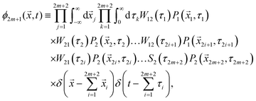 | (6) |
for a positive integer
m ≥ 0. Similarly, for an even number of switching events (particle ends up in phase 1 at time
t) the probability density of particle's position becomes (
m ≥ 0)
| | 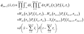 | (7) |
Therefore, using eqn (5)–(7) the probability density function particle's position ![[x with combining right harpoon above (vector)]](https://www.rsc.org/images/entities/i_char_0078_20d1.gif) at time t is
at time t is
| |  | (8) |
The summation on the right-hand side
(8) can be evaluated in the Fourier–Laplace transform defined by,
| |  | (9) |
where
s and
![[k with combining right harpoon above (vector)]](https://www.rsc.org/images/entities/i_char_006b_20d1.gif)
, respectively, are the conjugate variables with respect to time
t and position
![[x with combining right harpoon above (vector)]](https://www.rsc.org/images/entities/i_char_0078_20d1.gif)
, and the overhead bar and tilde, respectively, denote the Fourier and Laplace transformed expressions. This gives
| |  | (10) |
for
| |  | (11) |
| |  | (12) |
Then, we perform the summation in
eqn (10), and this gives Fourier–Laplace transformed probability density function:
| |  | (13) |
The above
eqn (13) is the characteristic function for the switching process in the Laplace space. The above formula is true for both Markovian and non-Markovian switching protocols. Similar results are found in ref.
59 and
91–94.
3 Effective diffusion coefficients
The propagator (13) is applicable to a wide range of switching processes. However, in several situations, it might be difficult to analytically invert the Fourier–Laplace transformed probability distribution (13). Nevertheless, the propagator (13) is useful to extract dynamical information for a general class of systems. Herein, we derive an exact expression for the effective diffusion coefficient valid for any two unbiased dynamical phases.
The n'th order position fluctuations along the one-dimensional coordinate x can be obtained by differentiating the Laplace transformed characteristic function  (13) with respect to kx and setting ki = 0 (for all i = x, y, z,…), and then, inverting the Laplace transform. For simplicity, in what follows we discuss one-dimensional processes. Therefore, the nth order position moment is
| |  | (14) |
The second derivative of the switching propagator (13) takes the form
| |  | (15) |
where prime indicates a derivative with respect to
k, and we used the zero-mean property

as well as normalization
![[P with combining tilde]](https://www.rsc.org/images/entities/i_char_0050_0303.gif) i
i(
k = 0,
t) = 1 for both phases. For brevity, we have introduced the functions
| |  | (16) |
| |  | (17) |
To obtain the long-time mean squared displacement and the effective diffusion coefficient, we have to consider the dominant pole in s as s → 0. First, we note that the term [1 − ![[W with combining tilde]](https://www.rsc.org/images/entities/i_char_0057_0303.gif) 12(s)
12(s)![[W with combining tilde]](https://www.rsc.org/images/entities/i_char_0057_0303.gif) 21(s)] in the denominator of both fractions in eqn (15) can be written for small s-values as‡
21(s)] in the denominator of both fractions in eqn (15) can be written for small s-values as‡
| |  | (18) |
by noting that
Wij(
t) denotes the probability density function and
![[W with combining tilde]](https://www.rsc.org/images/entities/i_char_0057_0303.gif) ij
ij(
s = 0) = 1. Since the second term in
eqn (15) has denominator [1 −
![[W with combining tilde]](https://www.rsc.org/images/entities/i_char_0057_0303.gif) 12
12(
s)
![[W with combining tilde]](https://www.rsc.org/images/entities/i_char_0057_0303.gif) 21
21(
s)]
2, this term will be the leading contribution at late times (
e.g. small
s). Hence, the long-time behaviour is given by
| |  | (19) |
where

. Upon inverting the Laplace transform, one finds that at long times, 〈
x2(
t)〉 ≈ 2
Defft, with the effective diffusion coefficient:
| |  | (20) |
Finally, from
eqn (17) we can calculate

by using the fact that
![[S with combining tilde]](https://www.rsc.org/images/entities/i_char_0053_0303.gif) i
i(0) = 〈
τi〉,
![[W with combining tilde]](https://www.rsc.org/images/entities/i_char_0057_0303.gif) ij
ij(0) = 1, as well as
| |  | (21) |
By combining the above we find the effective diffusion coefficient
| |  | (22) |
This expression is valid for any two symmetric processes with mean squared displacements 〈
x2(
t)〉
i (
i = 1, 2), for any switching protocol as long as the mean waiting times are well-defined 〈
τi〉 < ∞. When the particle is immobile in one of the phases,
e.g., 〈
x2(
t)〉
2 = 0, and the waiting time in the first phase is exponential, we recover the results obtained in ref.
95. When both phases are diffusive and the waiting times exponential, we recover existing results from models with switching diffusion coefficients.
74
In the case of intermittent active systems where the motion is interspersed with passive periods, we can use the above general formula (22) together with the known expression for the mean squared displacement of an active particle to obtain the effective diffusion coefficient. We let phase 1 correspond to the active phase, and phase 2 to the passive Brownian motion. Active particles are characterized by a persistence time τp, and the mean squared displacement takes the form96,97
| | | 〈x2(t)〉1 = 2v2τp[t + τp(e−t/τp − 1)], | (23) |
where
v is the self-propulsion speed. As the persistence time becomes smaller, a passive-like behaviour appears. Hence, active–passive switching can be thought of as the motion of an active particle that switches from the persistent motion, to less persistent motion, for example as part of an intermittent search strategy.
The passive phase is diffusive with 〈x2(t)〉2 = 2Dt where the passive diffusion coefficient is D. Eqn (22) then gives
| | 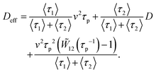 | (24) |
We note here that while the long-time effective diffusion coefficient of the active particle without passive phases would have been simply
v2τp, the long-time diffusion in the presence of switching also depends on the transient behavior coming from the mean squared displacement of the active phase,
eqn (23). While this transient is irrelevant at late times in the absence of switching, the recurrent restarts of the active phase make it relevant at late times once switching is considered. The above calculation remains general, and is valid for any waiting time density
W12(
t) in the active phase.
Therefore, a relevant question is how the choice of distribution of the active phase durations affects the effective diffusion coefficient. Since ![[W with combining tilde]](https://www.rsc.org/images/entities/i_char_0057_0303.gif) 12(τp−1) = 〈e−τ/τp〉, we note that by Jensen's inequality, we have
12(τp−1) = 〈e−τ/τp〉, we note that by Jensen's inequality, we have ![[W with combining tilde]](https://www.rsc.org/images/entities/i_char_0057_0303.gif) 12(τp−1) ≥ e−〈τ1〉/τp. At fixed mean durations of the active phase, this inequality is saturated only by the deterministic case W12(τ) = δ(τ − 〈τ1〉). Hence, at fixed durations of the two phases, the effective diffusivity is always smallest when the duration in the active phase is deterministic:
12(τp−1) ≥ e−〈τ1〉/τp. At fixed mean durations of the active phase, this inequality is saturated only by the deterministic case W12(τ) = δ(τ − 〈τ1〉). Hence, at fixed durations of the two phases, the effective diffusivity is always smallest when the duration in the active phase is deterministic:
| | | Deff[W] ≥ Deff[δ] ≡ Dmineff. | (25) |
Hence, fluctuations in the active phase durations are needed for effective spatial exploration.
Furthermore, since ![[W with combining tilde]](https://www.rsc.org/images/entities/i_char_0057_0303.gif) 12(s) ≤ 1 by monotonicity of integrals, we also have the upper bound
12(s) ≤ 1 by monotonicity of integrals, we also have the upper bound
| |  | (26) |
Hence, the effective diffusion coefficient is bounded as
Dmineff ≤
Deff ≤
Dmaxeff, with the explicit expressions given above
(25) and (26).
To illustrate the above results, we specifically consider the case when the active durations are drawn from a gamma distribution:
| |  | (27) |
where
Γ(·) is the Gamma-function. Its Laplace transform reads
| |  | (28) |
From this, the effective diffusion coefficient can be easily obtained from
eqn (24). We note that in this case, the dependence on the duration of the passive Brownian phase enters only through its first moment, and is insensitive to further details of the distribution
W21(
τ).
Fig. 2a shows the mean squared displacement obtained numerically together with the theoretical prediction [i.e., eqn (24) with (28)], verifying that the system's long-time behaviour will be diffusive with the effective diffusion coefficient Deff(22).
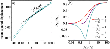 |
| | Fig. 2 (a) Mean squared displacement of an active run-and-tumble particle intermittently switching to a passive phase. Active durations are drawn from a gamma distribution (27) with shape index γ = 3. The dashed line shows theoretical prediction based on the effective diffusion coefficient [i.e., eqn (24) with (28)], while circles show numerical simulation data. For simplicity, the passive phases have deterministic duration 〈τ2〉 = 1/2. Remaining parameters used are v = 1, D = 1, τp = 0.5. (b) Effective diffusivity rescaled with DRT ≡ v2τp as a function of the ratio of active durations to passive durations, again for the case when active durations are drawn from a gamma distribution (27) with shape index γ = 3. In this case, we have set D/DRT = 0.1, so that passive phases are slow compared to the active motion. | |
Fig. 2b shows the effective diffusivity rescaled with the late-time pure run-and-tumble diffusion coefficient DRT ≡ v2τp, as a function of the ratio 〈τ1〉/〈τ2〉.
4 Model: active particles with intermittent passive phases
Section 2 discusses the framework of modelling processes switching between two arbitrary homogeneous dynamical phases. While general properties of such systems can be studied for symmetric processes, such as the effective diffusion coefficients in Section 3, the framework is also capable of handling more involved processes with bias. In this section, we consider in detail the case of a (potentially biased) run and tumble particle (RTP) that intermittently switches to passive Brownian motion (see Fig. 3).
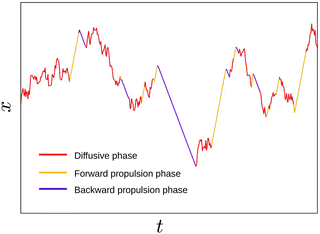 |
| | Fig. 3 Trajectory of a generalized run-and-tumble particle (orange and blue) with intermittent passive phases (red). | |
Let us consider the dynamics of an overdamped self-propelled particle in one dimension. Similar to the dynamics of the light-activated Janus particles,58 this particle has three phases of motion: (i) a forward propulsion with a speed vf, when irradiated by a UV light; (ii) a backward propulsion with a speed vb when irradiated by a green light; and (iii) a diffusive motion in the absence of light. Mathematically, the following equations model these phases:
| |  | (29) |
where
vb,f ≥ 0, and
η(
t) is a delta-correlated Gaussian white noise with zero mean: 〈
η(
t)
η(
t′)〉 =
δ(
t −
t′) and
D is the diffusion coefficient for the phase (iii).
We define the following switching mechanism between the three phases. The switching between the forward to backward propulsion and backward to forward propulsion (i.e., switching between UV and green light, and vice versa, respectively) happens at a rate αfb and αbf, respectively. The switching from the active propulsion phase to the passive diffusive phase, (i.e., any light being turned off) occurs at a rate ![[r with combining macron]](https://www.rsc.org/images/entities/i_char_0072_0304.gif) ap; while the switching from the passive to the active phase, (i.e., any light being turned on) occurs at a rate
ap; while the switching from the passive to the active phase, (i.e., any light being turned on) occurs at a rate ![[r with combining macron]](https://www.rsc.org/images/entities/i_char_0072_0304.gif) pa. Notice that we assume that when the lights are turned on, the particle can be either exposed to the UV or green light with equal probability. Furthermore, for simplicity, we consider a case where the particle always starts from the origin x = 0 at time t = 0 from any one of the active phases with equal probability.
pa. Notice that we assume that when the lights are turned on, the particle can be either exposed to the UV or green light with equal probability. Furthermore, for simplicity, we consider a case where the particle always starts from the origin x = 0 at time t = 0 from any one of the active phases with equal probability.
It is always convenient to define a characteristic length – ![[small script l]](https://www.rsc.org/images/entities/char_e146.gif) ≡ vf/αfb and a time-scale
≡ vf/αfb and a time-scale  . Then, eqn (29) can be expressed in the dimensionless variables x′ = x/
![[small script l]](https://www.rsc.org/images/entities/char_e146.gif) and
and  , and dimensionless (rescaled) diffusion coefficient
  . For convenience, we drop prime from these quantities, and write
| |  | (30) |
where
θ ≡
vb/
vf measures the asymmetry in the backward to forward speed. The noise is again delta-correlated in time 〈
η(
t1)
η(
t2)〉 =
δ(
t1 −
t2). In the dimensionless units, the relative switching between backward to forward motion occurs at a rate
A =
αbf/
αfb, and active–passive switching rates become
rap and
rpa.
In the following sections, we investigate this three-phase dynamics using the general switching formalism. To this end, we divide the dynamics eqn (30) into (1) an active phase where the particle switches between a forward propulsion state and a backward propulsion state; and (2) a passive diffusive phase. The active phase, a generalized version of the one-dimensional RTP, is itself an example of a switching process, which we first analyze in the following subsection.
4.1 Generalized run-and-tumble particles in one dimension
Several interesting extensions of the symmetric run-and-tumble particle have been considered over the years, including non-uniform and anisotropic tumbles.98–100 Here, we apply the above framework to the case of a run-and-tumble process in one dimension with biased run speeds,101 before subsequently including intermittent passive phases.
Here, we discuss the scenario (1). The forward and backward propulsion are given by eqn (30) (top two lines), they have the respective propagators,
| | | Pb(x, t) = δ(x − θt), | (32) |
which in the Fourier–Laplace space read:
| |  | (33) |
| |  | (34) |
Suppose the particle begins in the forward phase. Using eqn (13) for the exponential switching rate A measuring relative rate with respect to forward-to-backward propulsion rate αfb, we have for the Fourier–Laplace transform of the distribution  :
:
| |  | (35) |
Similarly, for the particle starting in the backward phase,
| |  | (36) |
We assume that the initial propulsion state of the active particle is chosen from the stationary state, pf = A/(1 + A) and pb = 1/(1 + A). Using this, the Fourier–Laplace transform of the position distribution becomes
| |  | (37) |
It is difficult to invert the above equation exactly to obtain a closed-form expression for the position distribution at all times. Nevertheless, the n'th moment of the position fluctuations can be obtained by using eqn (14). It turns out that the RTP is characterized by a non-zero mean,
| |  | (38) |
as expected. Interestingly, the mean vanishes when
A =
θ. We call this the ‘unbiased limit’ of the generalized RTP, where it has a zero mean in spite of having different velocities in the forward and backward propulsion phases. More precisely, the particle spends less time in the propulsion state with higher velocity, and more time in the lower velocity state, such that there is no net drift. This can be intuitively understood as follows. The system is initialized from the stationary probabilities of its forward and backward propulsion states, thus, at any time
t, the average-time spent by the particle in the forward and backward phase, respectively, is
At/(1 +
A) and
t/(1 +
A), which amounts to the total displacements in the respective phase
At/(1 +
A) and
Aθt/(1 +
A), respectively. The sum of these two displacements leads to
(38). Interestingly, the mean vanishes for
A =
θ. Notice that this is different from the ‘standard RTP’ limit (
i.e.,
A =
θ = 1), where again the mean is zero.
The variance σ(t)2 ≡ 〈x2(t)〉 − 〈x(t)〉2 is obtained as,
| |  | (39) |
Therefore, similar to the usual RTP, the variance shows two dynamical regimes depending on the value of
τRT ≡ min(1,
A−1),
| |  | (40) |
where
veff and
DRT denote the effective velocity of the fluctuations,
| |  | (41) |
and the diffusion coefficient
| |  | (42) |
respectively.
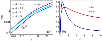
Fig. 4a discusses
σ2(
t) for different values of
A showing the ballistic and diffusive regimes of the variance.
Fig. 4b displays
veff and
DRT as functions of
A. Both are zero in the limits
A → 0 and
A → ∞, as in these limits, the particle is almost deterministic with very few tumbling events. However, at the intermediate values of
A,
veff and
Deff reach a maximum at
A = 1 and
A = 1/2, respectively. The magnitude of the relative propulsion speed
θ does not influence the position of the maximum; however, it determines their respective maximum values.
 |
| | Fig. 4 Position fluctuations of a generalized RTP. (a) The variance of the particle for different values of A, crosses over from an initial ballistic phase to a late time diffusive phase at times t ∼ min(1, A−1). Color intensity increases with increasing value of the relative switching rate between backward to forward motion, A. (b) The variation of the effective velocity veff of the fluctuations and the effective diffusivity Deff with respect to A. For both plots θ = 1. | |
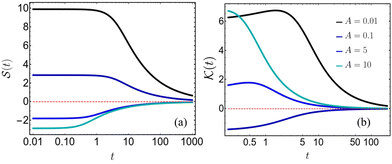
We further compute the skewness,  of the position distribution, which quantifies the asymmetry of a distribution with respect to its mean value. The skewness vanishes over long time, with the leading order behaviour,
| |  | (43) |
The distribution becomes symmetric about its mean from a positively or negatively skewed distribution depending on
A > 1 or
A < 1. This is because for
A < 1, the time spent in the positive velocity phase is lesser compared to the time spent in the negative velocity phase. This is shown in
Fig. 5a for different values of
A.
 |
| | Fig. 5 Approach of the position fluctuations of generalized run and tumble particle to a Gaussian distribution. Skewness (a) and kurtosis (b) as a function of time t. Color intensity increases with increasing value of A. We fix the speed asymmetry in backward to forward motion to θ = 1. | |
Moreover, excess kurtosis,  can also be computed exactly and goes to zero as,
| |  | (44) |
The distribution thus tends to a Gaussian distribution from a platykurtic (negative kurtosis) or a leptokurtic side (positive kurtosis) for

and

respectively, as shown in
Fig. 5b. For very small or large
A, the particle spends more time moving in one direction, thus the distribution approaches the corresponding normal distribution from one which is more sharply peaked, leading to the positive kurtosis. The negative kurtosis for intermediate values of
A, on the other hand, occurs due to the competition of the time spent in the forward and backward motion, which are of the same order, causing more fluctuations resulting in the approach to the corresponding Gaussian distribution to happen from a flatter side.
4.2 Run-and-tumble particles with intermediate passive phases
In the previous Section 4.1, we discuss the case of an active particle in one dimension switching its directions (forward ↔ backward), i.e., the generalized RTP. Herein, following the framework developed in Section 2, we extend our analysis to a case of a particle switching its motion between the generalized RTP and a passive (Brownian) dynamics. For convenience, we consider a case in which the particle is initialized in the generalized RTP phase (we refer to this phase as ‘phase 1’). The Fourier–Laplace transform of the propagator reads| |  | (45) |
where  is given in (37). ‘Phase 2’, on the other hand, is a passive diffusion phase with its propagator in the Fourier–Laplace space:
| |  | (46) |
The general formula for the Fourier–Laplace transform of the position distribution (13) for waiting times being governed by Poisson distribution (Wij(t) ≡ rije−rijt), is
| |  | (47) |
Thus, using the aforementioned
 (45)
(45) and
 (46)
(46) we find

exactly [see Appendix A]. The expression of

is rather long, and we relegate it to the Appendix A. Further, it is also difficult to invert this Fourier–Laplace transformed expression. Nonetheless, we compute the first four cumulants to understand the statistics of this switching process (
i.e., generalized RTP ↔ Brownian dynamics).
Employing (14) for eqn (47), we compute the first position moment:
| |  | (48) |
The mean position is independent of the diffusion coefficient,
D, of the passive phase, since the only drift comes due to the particle's active motion.
At short-time, the mean position retains exactly the same property as the generalized RTP (38):
| |  | (49) |
This can be understood as we consider that the particle always begins in the active phase, and in the short-time regime,
t ≪ (
rap), there are typically no switching events. In the long-time regime, though there have been an appreciable number of switching events, the mean is the same as
eqn (49), however, now weighed by the average time spent in the active phase:
| |  | (50) |
The variance or the second cumulant captures the position fluctuations. In the following, we discuss its asymptotic behaviours [however, the full-time dependent form can be calculated using (14) for eqn (47)]:
| |  | (51) |
where the effective diffusive coefficient is
| |  | (52) |
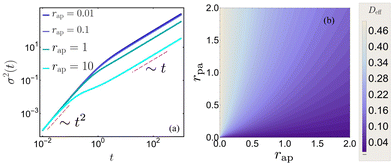
Fig. 6a displays the time evolution of the variance for different values of rap, indicating the short-time ballistic and long-time diffusive regime [see eqn (51)].
 |
| | Fig. 6 Position fluctuation of a generalized run-and-tumble particle with intermediate passive phases. (a) Variance as a function of time t. The color intensity increases with active to passive switching rate rap. We fix rpa = 1. The red and magenta dashed lines, respectively, indicate the short-time ballistic and long-time diffusive behaviour. (b) Effective diffusion coefficient in the (rap, rpa) plane. Here, we fix A = 1 and D = 0.01. | |
To investigate how the effective diffusion coefficient Deff(52) changes with respect to the switching rates, we analyse Deff in the (rap, rpa) plane. To this end, we note that, in the limit rap → 0, the effective diffusion coefficient Deff → DRT. Moreover, since we consider the diffusion coefficient in the active phase DRT is larger than the diffusive phase (so that the diffusive phase is slower than the active phase), the effective diffusion coefficient of the particle is always peaked at the line rap = 0. For finite values of rap, Deff increases with the increase in rpa as the time spent in the diffusive phases decreases. This is illustrated in Fig. 6b.
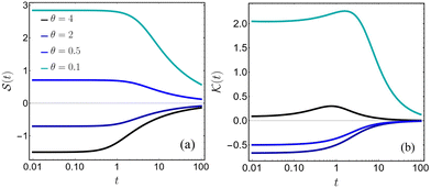
For the higher cumulants, we specifically focus on the case where A = θ (unbiased limit of the generalized RTP). It turns out that the skewness goes to zero in the long-time limit as
| |  | (53) |
indicating the resulting distribution to be a symmetric one. Depending on the case, if
θ is smaller or larger than unity, the distribution becomes symmetric from a positively or a negatively skewed distribution, respectively (
Fig. 7a). Thus, though temporal-scaling remains unchanged compared to the generalized RTP model [
cf.(43)], the prefactor is modified.
 |
| | Fig. 7 Approach of the position fluctuations of generalized run and tumble particle to a Gaussian distribution with intermediate passive phases. Skewness (a) and kurtosis (b) as a function of time t. Here, we fix rpa = 0.01, rap = 1, D = 0.01 and different values of θ = A. | |
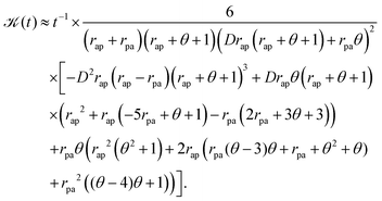
The kurtosis can also be exactly computed and the leading order behaviour at long-time limit is given by,
| |  | (54) |
The
t−1 – coefficient's sign determines if the kurtosis approaches Gaussian from a platykurtic or leptokurtic distribution. For very small or large
θ, the particle when in the active phase spends more time in moving in one of the run phases, leading to sharper distribution than the corresponding Gaussian distribution at a long-time; leading to

approach zero from the positive side. For intermediate
θ, on the other hand, the competition between the forward and backward runs is stronger, leading to stronger position fluctuations causing the distribution to approach Gaussianity from the negative side. This is shown in
Fig. 7b for different values of
θ.
5 Time evolution of the position distribution
In the previous section, we discussed the cumulants of the two different switching processes. Here, we analyse the time-dependence of the density of a large number of non-interacting active particles with intermittent passive phase. For simplicity, we specialized to the case of the standard RTP (i.e., A = θ = 1) with rap = rpa = r. The Fourier–Laplace transform of the probability distribution (47) in this case has a simpler form:| |  | (55) |
Since the above (55) Fourier–Laplace transform is difficult to invert, we first discuss the time evolution behavior of the position distribution as seen from numerical simulations. Thereafter, we perform some asymptotic analysis.
Let us first discuss the time evolution of the position distribution qualitatively. From Fig. 8, we see that at short-time t ≪ {1, r−1}, the distribution has two different dynamical regions characterized by an RTP like behavior till x = ±t, followed by non-trivial tail behavior, which we find asymptotically in eqn (66); at x = ±t, there are two Dirac-delta function-like peaks which can be attributed to the particles that have not changed propulsion states, or switched to passive state, in time t. With the increase in time, this peak vanishes, and the two dynamical regions combine, eventually becoming Gaussian-like at long-time, as also predicted from the cumulant analysis in the previous sections, see Fig. 5. In the following, we also find the asymptotic distribution at very long-time, starting from eqn (55).
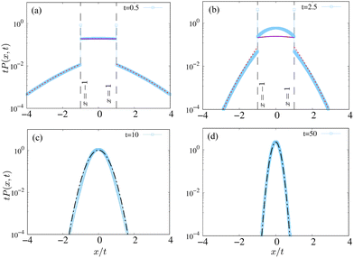 |
| | Fig. 8 Time evolution of the position distribution of the standard run-and-tumble particle with intermittent passive phases. Symbols: numerical simulations. (a) and (b) Correspond to short-time distributions for t ≪ (r−1, γ−1), and γ−1 < t < r−1 respectively. The red dashed lines denote the short-time analytical prediction (66) for the tails, while the solid purple lines denote eqn (65). The dashed vertical lines denote the position of the delta function (57). The dot-dashed lines in (c) and (d) denote the large-time Gaussian behavior (69). Here, we fix D = 1 and r = 0.1. | |
5.1 Short-time distribution
To understand the short-time distribution t ≪ (r−1, α−1), we perform a trajectory-based calculation based on the number of tumbles and switches that the particle has undergone. We write the distribution as a perturbative series in the active–passive switching rate r and the RTP's tumbling rate αfb = αbf = α = 1:| |  | (56) |
where P(n,m)(x,t) denotes the contributions of trajectories with n switches and m tumbles and is of the order  . For time t ≪ (α−1, r−1), the first few terms in the above series is expected to provide a good description of the short-time distribution. Let us systematically compute the first few order contributions.
For trajectories that have undergone neither tumbling nor switching events, we have the following contribution:
| |  | (57) |
where we assumed that the particle starts from
x = 0 in the active phase
j = ±1 with equal probability 1/2. Notice that the above contribution
(57) is non-zero only at
x = ±
t, and its weight decreases as time increases.
Fig. 8a and b demonstrates these delta functions at
x/
t = ±1.
Next for trajectories with one switch but no tumbling events, i.e., the contribution of  , we have
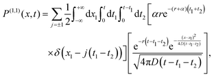
| | 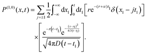 | (58) |
The terms in the first squared brackets denote the probability that the particle, starting from
x = 0 in the active state
j, does not undergo any tumbling or switching event till time
t1 and reaches to
x1 =
jt1, then, it switches to the passive-phase. The terms in the second squared brackets denotes the probability that once the particle in the passive-phase it stays in the same phase in the remaining time
t −
t1 and reaches to the position
x. The integration
(58) over
x1 gives
| |  | (59) |
An exact closed form of the above integral cannot be obtained. Nevertheless, the integration can be performed numerically.
Next we consider terms of order  . This comes from trajectories which have undergone one tumbling event at time t1 before switching to the passive-phase at time t1 + t2,
| |  | (60) |
where
x1 denotes the distance travelled till time
t1 +
t2, and the second brackets correspond to the particle staying in the passive phase in the remaining time
t −
t1 −
t2. The integral
(60) over
x1 can be performed, and it gives
| |  | (61) |
Now let us evaluate the contribution from trajectories, which have undergone tumbling events, but have never switched to the passive phase. Such contributions P(0,1)(x,t) is given by
| |  | (62) |
The right-hand side of above equation can be understood as follows: e
−rt accounts for no switching in the entire duration
t, the factor
αe
−αt1 denotes that the particle undergoes the first tumble event at
t1; e
−α(t−t1) denotes that the particle does not undergo any further tumbling event in the remaining time
t −
t1, and finally the delta function denotes the position of the particle having started in a state
j. Performing the integral over
t1, we get
| |  | (63) |
Similarly, for two tumbles (and no switching event), the contribution to the probability distribution is
| |  | (64) |
Analogously, one can find higher-order terms systematically. However, to understand the observed distributions we truncate the series (56) for short-time as
| |  | (65) |
Note that the Heaviside theta functions in both
P(0,1) and
P(0,2) indicate that the contributions from these trajectories remain confined with |
x| <
t. Thus, the contribution to the distribution |
x| >
t comes from trajectories with at least one switch, and for short-time the tails' distribution can be approximated as
| | | Ptail(x,t) ≈ P(0,1)(x,t) + P(0,2)(x,t). | (66) |
Fig. 8 shows the comparison of tails' analytical results
(66) with the numerical simulations, and it shows a good agreement.
The inner region |x| < t, however, requires the contribution from all the terms on the right-hand side of eqn (65). Fig. 8a and b show the comparison of analytical results [eqn (65) and (66)] with the numerical simulation for the inner region. We find that α−1 < t < r−1, we see that the inner region shows a deviation. This is due to the fact that the particle's trajectories have undergone multiple tumbles without any switching events, and higher-order terms in eqn (65) are required.
5.2 Long-time distribution
The behaviour of the distribution near the tails is dominated by contributions coming from small-k behaviour. In this limit, the Fourier–Laplace transform simplifies eqn (55) to,| |  | (67) |
Additionally, in the limit s → 0, which corresponds to the long-time behaviour, the above eqn (67) simplifies to:| |  | (68) |
which by inverting the Fourier and Laplace transform, leads to a diffusive Gaussian scaling of the tails over long-time:| |  | (69) |
Fig. 8c and d show a good agreement of the Gaussian description (69) with the numerical simulation for longer times (t ≫ r−1).
6 Summary
We analyzed a dynamical process characterized by a stochastic switching mechanism. By employing a trajectory-based approach, we derived the Fourier–Laplace transform of the position distribution for a particle undergoing such switching dynamics, with arbitrary waiting times. We calculated the generalized diffusion coefficient for this system, assuming the waiting time distributions possess a finite mean. We then applied this framework to an example of an active particle exhibiting intermittent diffusive phases, where we computed the exact expressions for the first few position cumulants. Additionally, we derived asymptotic expressions for the tails of the probability density function at all times, and our results were corroborated by numerical data.
Although our study focuses on one-dimensional processes, the general formulas we developed are applicable to any number of dimensions and can be utilized to investigate switching processes in higher-dimensional settings. The first-passage properties of these active processes display intriguing characteristics, particularly when compared to standard diffusion.102 It would be interesting to explore whether intermittent diffusive phases could potentially enhance the first-passage times of active particles. Furthermore, another promising direction for future research is to examine the role of confining potential,103 many interacting particles, and stochastic resetting64 on the distribution of switching processes. Finally, there are multiple intriguing extensions to more than two dynamical phases. Processes that switch between N dynamical phases can often be decomposed into multiple two-phase systems. For such decomposition, one has to modify the rates of switching from one phase to another and vice versa in the effective sense.104 This is an interesting topic, and could be considered for future research. In the future, repeated application of eqn (13) could be used to study such higher-order switching dynamics. In such cases, one could also consider cases where switching is coupled to the system's state, e.g., by only allowing switching transitions in a subset of the phases. Furthermore, in this paper, we discussed switching mechanism by an instantaneous protocol, our results, however, can be generalized to non-instantaneous switching protocols by introducing an additional intermediate phase; such generalization and application of different temporal distribution of intermediate phase will be considered for future research.
Data availability
No external data were used for the preparation of the manuscript, all the relevant details can be found in the manuscript.
Conflicts of interest
There are no conflicts to declare.
Appendices
A Exact expressions used in the main text
In this section we provide the exact expressions for some of the expressions whose asymptotes or derivatives have been shown in the main text, namely skewness and kurtosis for the generalized RTP supplementing Section 4.1 and the generating function of the RTP with intermediate passive phases used in Section 4.2.
A.1 Generalized RTP.
Using the generating function eqn (37) and (14), the skewness of the position of the generalized RTP is given as,| |  | (70) |
which at large time, reduces to eqn (43). Similarly, from the fourth moment of the position distribution, the kurtosis can be obtained as| |  | (71) |
The above equation at long-times reduces to eqn (44).
A.2 RTP with intermittent passive phases.
The Fourier–Laplace transform of the distribution is given by,| |  | (72) |
Here,| | | H ≡ (A + 1)(A(k + i(rap + s)) + (k + i(rap + s + 1))(ikθ + rap + s)). | (73) |
Acknowledgements
K. S. O. acknowledges support from the Deutsche Forschungsgemeinschaft (DFG) within the project LO 418/29-1. D. G. acknowledges support from the Nordita fellowship program. Nordita is partially supported by Nordforsk. The authors thank the anonymous reviewers for their valuable suggestions that have improved the content and presentation of the manuscript. We thank University of Göttingen Open Access Policy for providing the open access charges of this manuscript.
Notes and references
-
G. G. Yin and C. Zhu, Hybrid switching diffusions, of Stochastic Modelling and Applied Probability, 2010, vol. 63 Search PubMed.
- P. C. Bressloff, J. Phys. A: Math. Theor., 2020, 53, 275003 CrossRef.
- G. Tucci, É. Roldán, A. Gambassi, R. Belousov, F. Berger, R. G. Alonso and A. J. Hudspeth, Phys. Rev. Lett., 2022, 129, 030603 CrossRef CAS PubMed.
- K. Schafer, Vet. Pathol., 1998, 35, 461–478 CrossRef CAS PubMed.
- J. Rombouts and L. Gelens, PLoS Comput. Biol., 2021, 17, e1008231 CrossRef CAS PubMed.
- J. M. Morales, D. T. Haydon, J. Frair, K. E. Holsinger and J. M. Fryxell, Ecology, 2004, 85, 2436–2445 CrossRef.
- T. Michelot and P. G. Blackwell, Methods Ecol. Evol., 2019, 10, 637–649 CrossRef.
- A. Sabri, X. Xu, D. Krapf and M. Weiss, Phys. Rev. Lett., 2020, 125, 058101 CrossRef CAS PubMed.
- M. Balcerek, A. Wyłomańska, K. Burnecki, R. Metzler and D. Krapf, New J. Phys., 2023, 25, 103031 CrossRef.
- L. Mirny, M. Slutsky, Z. Wunderlich, A. Tafvizi, J. Leith and A. Kosmrlj, J. Phys. A: Math. Theor., 2009, 42, 434013 CrossRef.
- C. Loverdo, O. Benichou, R. Voituriez, A. Biebricher, I. Bonnet and P. Desbiolles, Phys. Rev. Lett., 2009, 102, 188101 CrossRef CAS PubMed.
- J. Buhl, D. J. Sumpter, I. D. Couzin, J. J. Hale, E. Despland, E. R. Miller and S. J. Simpson, Science, 2006, 312, 1402–1406 CrossRef CAS PubMed.
- G. Ariel, Y. Ophir, S. Levi, E. Ben-Jacob and A. Ayali, PLoS One, 2014, 9, e101636 CrossRef PubMed.
-
E. Barone and G. Patterson, arXiv, 2023, preprint, arXiv:2311.14847, DOI:10.1103/PhysRevE.109.054609.
- K. S. Olsen, L. Angheluta and E. G. Flekkøy, Phys. Rev. Res., 2022, 4, 043017 CrossRef CAS.
- G. Tkačik and W. Bialek, Annu. Rev. Condens. Matter Phys., 2016, 7, 89–117 CrossRef.
- M. Caraglio, H. Kaur, L. J. Fiderer, A. López-Incera, H. J. Briegel, T. Franosch and G. Muñoz-Gil, Soft Matter, 2024, 20, 2008–2016 RSC.
- M. Nasiri, H. Löwen and B. Liebchen, Europhys. Lett., 2023, 142, 17001 CrossRef CAS.
- S. Ramaswamy, Annu. Rev. Condens. Matter Phys., 2010, 1, 323–345 CrossRef.
- M. C. Marchetti, J.-F. Joanny, S. Ramaswamy, T. B. Liverpool, J. Prost, M. Rao and R. A. Simha, Rev. Mod. Phys., 2013, 85, 1143 CrossRef CAS.
- J. Elgeti, R. G. Winkler and G. Gompper, Rep. Prog. Phys., 2015, 78, 056601 CrossRef CAS PubMed.
- C. Bechinger, R. Di Leonardo, H. Löwen, C. Reichhardt, G. Volpe and G. Volpe, Rev. Mod. Phys., 2016, 88, 045006 CrossRef.
- H. C. Berg, Annu. Rev. Biophys. Bioeng., 1975, 4, 119–136 CrossRef CAS PubMed.
- S. J. Ebbens and J. R. Howse, Soft Matter, 2010, 6, 726–738 RSC.
- D. Helbing, I. Farkas and T. Vicsek, Nature, 2000, 407, 487–490 CrossRef CAS PubMed.
- L. Caprini, A. Ldov, R. K. Gupta, H. Ellenberg, R. Wittmann, H. Löwen and C. Scholz, Commun. Phys., 2024, 7, 52 CrossRef.
- I. S. Aranson, D. Volfson and L. S. Tsimring, Phys. Rev. E: Stat., Nonlinear, Soft Matter Phys., 2007, 75, 051301 CrossRef PubMed.
- N. Kumar, H. Soni, S. Ramaswamy and A. Sood, Nat. Commun., 2014, 5, 4688 CrossRef CAS PubMed.
- I. Santra, U. Basu and S. Sabhapandit, Phys. Rev. E, 2021, 104, L012601 CrossRef CAS PubMed.
- I. Santra, U. Basu and S. Sabhapandit, Soft Matter, 2021, 17, 10108–10119 RSC.
- K. S. Olsen, Phys. Rev. E, 2021, 103, 052608 CrossRef CAS PubMed.
- S. Das and U. Basu, J. Stat. Mech.: Theory Exp., 2023, 2023, 063205 CrossRef.
- D. A. Krasky and D. Takagi, J. Stat. Mech.: Theory Exp., 2018, 2018, 103201 CrossRef.
- D. Frydel, Phys. Fluids, 2022, 34, 027111 CrossRef CAS.
- T. Demaerel and C. Maes, Phys. Rev. E, 2018, 97, 032604 CrossRef CAS PubMed.
-
F. Peruani and D. Chaudhuri, arXiv, 2023, preprint, arXiv:2306.05647, DOI:10.48550/arXiv.2306.05647.
- E. Perez Ipiña, S. Otte, R. Pontier-Bres, D. Czerucka and F. Peruani, Nat. Phys., 2019, 15, 610–615 Search PubMed.
- D. Arcizet, B. Meier, E. Sackmann, J. O. Rädler and D. Heinrich, Phys. Rev. Lett., 2008, 101, 248103 CrossRef PubMed.
-
M. Caraglio, H. Kaur, L. J. Fiderer, A. López-Incera, H. J. Briegel, T. Franosch and G. Muñoz-Gil, arXiv, 2023, preprint, arXiv:2311.16692, 10.1039/D3SM01680C.
- P. Maiuri, J.-F. Rupprecht, S. Wieser, V. Ruprecht, O. Bénichou, N. Carpi, M. Coppey, S. De Beco, N. Gov and C.-P. Heisenberg,
et al.
, Cell, 2015, 161, 374–386 CrossRef CAS PubMed.
- D. Breoni, F. J. Schwarzendahl, R. Blossey and H. Löwen, Eur. Phys. J. E: Soft Matter Biol. Phys., 2022, 45, 83 CrossRef CAS PubMed.
- S. Bazazi, F. Bartumeus, J. J. Hale and I. D. Couzin, PLoS Comput. Biol., 2012, 8, e1002498 CrossRef CAS PubMed.
- M. Stojan-Dolar and E. W. Heymann, Int. J. Primatol., 2010, 31, 677–692 CrossRef PubMed.
- F. Bartumeus, Oikos, 2009, 118, 488–494 CrossRef.
- D. L. Kramer and R. L. McLaughlin, Am. Zool., 2001, 41, 137–153 Search PubMed.
- A. D. Wilson and J.-G. J. Godin, Behav. Chem. Ecol., 2010, 21, 57–62 CrossRef.
-
A. P. Antonov, L. Caprini, C. Scholz and H. Löwen, arXiv, 2024, preprint, arXiv:2404.06615, DOI:10.1103/PhysRevLett.133.198301.
-
A. Datta, C. Beta and R. Großmann, arXiv, 2024, preprint, arXiv:2406.15277, DOI:10.48550/arXiv.2406.15277.
-
T. Jamali, arXiv, 2020, preprint, arXiv:2012.14155, DOI:10.48550/arXiv.2012.14155.
- S. Hahn, S. Song, G.-S. Yang, J. Kang, K. T. Lee and J. Sung, Phys. Rev. E, 2020, 102, 042612 CrossRef CAS PubMed.
- W. Trouilloud, A. Delisle and D. L. Kramer, Anim. Behav., 2004, 67, 789–797 CrossRef.
- T. E. Higham, P. Korchari and L. D. McBrayer, Biol. J. Linn. Soc., 2011, 102, 83–90 CrossRef.
- A. E. Hafner, L. Santen, H. Rieger and M. R. Shaebani, Sci. Rep., 2016, 6, 37162 CrossRef CAS PubMed.
-
A. Datta, S. Beier, V. Pfeifer, R. Großmann and C. Beta, arXiv, 2024, preprint, arXiv:2408.02317, DOI:10.48550/arXiv.2408.02317.
- I. Buttinoni, G. Volpe, F. Kümmel, G. Volpe and C. Bechinger, J. Phys.: Condens. Matter, 2012, 24, 284129 CrossRef PubMed.
- J. Palacci, S. Sacanna, A. P. Steinberg, D. J. Pine and P. M. Chaikin, Science, 2013, 339, 936–940 CrossRef CAS PubMed.
- I. Buttinoni, J. Bialké, F. Kümmel, H. Löwen, C. Bechinger and T. Speck, Phys. Rev. Lett., 2013, 110, 238301 CrossRef PubMed.
- H. R. Vutukuri, M. Lisicki, E. Lauga and J. Vermant, Nat. Commun., 2020, 11, 2628 CrossRef CAS PubMed.
- K. Singwi and A. Sjölander, Phys. Rev., 1960, 119, 863 CrossRef CAS.
- P. Chaudhuri, L. Berthier and W. Kob, Phys. Rev. Lett., 2007, 99, 060604 CrossRef PubMed.
- R. Zwanzig, Chem. Phys. Lett., 1989, 164, 639–642 CrossRef CAS.
- R. Zwanzig, J. Chem. Phys., 1992, 97, 3587–3589 CrossRef CAS.
- R. Zwanzig, Acc. Chem. Res., 1990, 23, 148–152 CrossRef CAS.
- M. R. Evans, S. N. Majumdar and G. Schehr, J. Phys. A: Math. Theor., 2020, 53, 193001 CrossRef.
- G. Mercado-Vásquez, D. Boyer, S. N. Majumdar and G. Schehr, J. Stat. Mech.: Theory Exp., 2020, 2020, 113203 CrossRef.
- I. Santra, S. Das and S. K. Nath, J. Phys. A: Math. Theor., 2021, 54, 334001 CrossRef.
- D. Gupta, C. A. Plata, A. Kundu and A. Pal, J. Phys. A: Math. Theor., 2020, 54, 025003 CrossRef.
- G. Mercado-Vásquez, D. Boyer and S. N. Majumdar, J. Stat. Mech.: Theory Exp., 2022, 2022, 093202 CrossRef.
- K. S. Olsen, D. Gupta, F. Mori and S. Krishnamurthy, Phys. Rev. Res., 2024, 6, 033343 CrossRef.
- K. S. Olsen and D. Gupta, J. Phys. A: Math. Theor., 2024, 57, 245001 CrossRef.
-
D. Frydel, arXiv, 2024, preprint, arXiv:2407.12213, DOI:10.1103/PhysRevE.110.024613.
- P. C. Bressloff, J. Phys. A: Math. Theor., 2017, 50, 133001 CrossRef.
- N. A. Baran, G. Yin and C. Zhu, Adv. differ. equ., 2013, 2013, 1–13 CrossRef.
- D. S. Grebenkov, Phys. Rev. E, 2019, 99, 032133 CrossRef CAS PubMed.
- D. S. Grebenkov, J. Phys. A: Math. Theor., 2019, 52, 174001 CrossRef.
- K. Goswami and R. Chakrabarti, Soft Matter, 2022, 18, 2332–2345 RSC.
- O. Bénichou, C. Loverdo, M. Moreau and R. Voituriez, Rev. Mod. Phys., 2011, 83, 81 CrossRef.
- P. C. Bressloff and J. M. Newby, Rev. Mod. Phys., 2013, 85, 135 CrossRef CAS.
- S. Rukolaine, J. Phys.: Conf. Ser., 2019, 044029 CrossRef.
- S. Rukolaine, Tech. Phys., 2018, 63, 1262–1269 CrossRef CAS.
- M. Hidalgo-Soria, E. Barkai and S. Burov, Entropy, 2021, 23, 231 CrossRef PubMed.
- S. Sadegh, E. Barkai and D. Krapf, New J. Phys., 2014, 16, 113054 CrossRef.
- M. Niemann, H. Kantz and E. Barkai, Phys. Rev. Lett., 2013, 110, 140603 CrossRef PubMed.
- N. Van Kampen, Phys. A, 1979, 96, 435–453 CrossRef.
-
P. C. Bressloff, arXiv, 2023, preprint, arXiv:2310.20502, DOI:10.1103/PhysRevE.109.024103.
- M. H. Davis, J. R. Stat. Soc.: Series B (Methodological), 1984, 46, 353–376 CrossRef.
-
T. R. Olivier Cappé and E. Moulines, Inference in Hidden Markov Models, Springer, New York, NY, 1st edn, 2005 Search PubMed.
- F. M. van Beest, S. Mews, S. Elkenkamp, P. Schuhmann, D. Tsolak, T. Wobbe, V. Bartolino, F. Bastardie, R. Dietz and C. von Dorrien,
et al.
, Sci. Rep., 2019, 9, 5642 CrossRef PubMed.
- J. Bechhoefer, New J. Phys., 2015, 17, 075003 CrossRef.
-
N. van Kampen, Stochastic Processes in Physics and Chemistry, Elsevier Science Publishers, Amsterdam, 1992 Search PubMed.
- F. Detcheverry, Europhys. Lett., 2015, 111, 60002 CrossRef.
- F. Thiel, L. Schimansky-Geier and I. M. Sokolov, Phys. Rev. E: Stat., Nonlinear, Soft Matter Phys., 2012, 86, 021117 CrossRef PubMed.
- L. Angelani, Europhys. Lett., 2013, 102, 20004 CrossRef CAS.
- C. Dieball, D. Krapf, M. Weiss and A. Godec, New J. Phys., 2022, 24, 023004 CrossRef.
- K. S. Olsen and H. Löwen, J. Stat. Mech.: Theory Exp., 2024, 2024, 033210 CrossRef.
- P. Romanczuk, M. Bär, W. Ebeling, B. Lindner and L. Schimansky-Geier, Eur. Phys. J.: Spec. Top., 2012, 202, 1–162 CAS.
- I. Santra, U. Basu and S. Sabhapandit, Phys. Rev. E, 2020, 101, 062120 CrossRef CAS PubMed.
- A. Villa-Torrealba, C. Chávez-Raby, P. de Castro and R. Soto, Phys. Rev. E, 2020, 101, 062607 CrossRef CAS PubMed.
- F. J. Sevilla, Phys. Rev. E, 2020, 101, 022608 CrossRef CAS PubMed.
- B. Loewe, T. Kozhukhov and T. N. Shendruk, Soft Matter, 2024, 20, 1133–1150 RSC.
- O. López and N. Ratanov, J. Appl. Probability, 2014, 51, 569–589 CrossRef.
-
U. Basu, S. Sabhapandit and I. Santra, arXiv, 2023, preprint, arXiv:2311.17854, DOI:10.48550/arXiv.2311.17854.
- A. Pototsky and H. Stark, Europhys. Lett., 2012, 98, 50004 CrossRef.
- Q. Yu, D. Zhang and Y. Tu, Phys. Rev. Lett., 2021, 126, 080601 CrossRef CAS PubMed.
Footnotes |
| † The authors contributed equally to this work. |
‡  |
|
| This journal is © The Royal Society of Chemistry 2024 |
Click here to see how this site uses Cookies. View our privacy policy here.  Open Access Article
 *a,
Kristian Stølevik
Olsen
 b and
Deepak
Gupta†
 *cd
*cd
 . The waiting time-intervals τ1, τ3, … (τ2, τ4, …), which correspond to a switch from phase 1 to phase 2 (phase 2 to phase 1), are drawn from the probability density function W12(τ) ≡ W1→2 (W21(τ) ≡ W2→1), see Fig. 1. Then, the survival probabilities S1(t) or S2(t), respectively, denote the probability that the particle starting from phase 1 or phase 2 has not switched to its complementary phase until time t. Mathematically, these read as

![[x with combining right harpoon above (vector)]](https://www.rsc.org/images/entities/i_char_0078_20d1.gif) 0 at time t0; this is denoted by P1(
0 at time t0; this is denoted by P1(![[x with combining right harpoon above (vector)]](https://www.rsc.org/images/entities/i_char_0078_20d1.gif) , t|
, t|![[x with combining right harpoon above (vector)]](https://www.rsc.org/images/entities/i_char_0078_20d1.gif) 0, t0) [or P2(
0, t0) [or P2(![[x with combining right harpoon above (vector)]](https://www.rsc.org/images/entities/i_char_0078_20d1.gif) , t|
, t|![[x with combining right harpoon above (vector)]](https://www.rsc.org/images/entities/i_char_0078_20d1.gif) 0, t0)], where
0, t0)], where ![[x with combining right harpoon above (vector)]](https://www.rsc.org/images/entities/i_char_0078_20d1.gif) is the particle's position at time t. Further, we assume no potential energy landscapes in either of these phases; therefore, the particle's dynamics in each phase depends on the distance covered from its initial location in time t − t0. Thus, we write
is the particle's position at time t. Further, we assume no potential energy landscapes in either of these phases; therefore, the particle's dynamics in each phase depends on the distance covered from its initial location in time t − t0. Thus, we write![[x with combining right harpoon above (vector)]](https://www.rsc.org/images/entities/i_char_0078_20d1.gif) −
− ![[x with combining right harpoon above (vector)]](https://www.rsc.org/images/entities/i_char_0078_20d1.gif) 0, t − t0) ≡ Pj(
0, t − t0) ≡ Pj(![[x with combining right harpoon above (vector)]](https://www.rsc.org/images/entities/i_char_0078_20d1.gif) −
− ![[x with combining right harpoon above (vector)]](https://www.rsc.org/images/entities/i_char_0078_20d1.gif) 0, t − t0|0,0) = Pj(
0, t − t0|0,0) = Pj(![[x with combining right harpoon above (vector)]](https://www.rsc.org/images/entities/i_char_0078_20d1.gif) , t|
, t|![[x with combining right harpoon above (vector)]](https://www.rsc.org/images/entities/i_char_0078_20d1.gif) 0, t0),
0, t0),![[x with combining right harpoon above (vector)]](https://www.rsc.org/images/entities/i_char_0078_20d1.gif) 0 = (0, 0,…), at time t = 0 in phase 1. Let the time-interval between the i'th and the (i + 1)'th switching event be τi+1, and the displacement in that time-interval be
0 = (0, 0,…), at time t = 0 in phase 1. Let the time-interval between the i'th and the (i + 1)'th switching event be τi+1, and the displacement in that time-interval be ![[x with combining right harpoon above (vector)]](https://www.rsc.org/images/entities/i_char_0078_20d1.gif) i+1. Then, the propagator accounts for the contributions arising from trajectories experiencing different numbers of switching events until time t.
i+1. Then, the propagator accounts for the contributions arising from trajectories experiencing different numbers of switching events until time t.![[x with combining right harpoon above (vector)]](https://www.rsc.org/images/entities/i_char_0078_20d1.gif) in time t, from a trajectory that has not experienced a single switching event until time t. This is given by
in time t, from a trajectory that has not experienced a single switching event until time t. This is given by![[x with combining right harpoon above (vector)]](https://www.rsc.org/images/entities/i_char_0078_20d1.gif) , t) ≡ S1(t)P1(
, t) ≡ S1(t)P1(![[x with combining right harpoon above (vector)]](https://www.rsc.org/images/entities/i_char_0078_20d1.gif) , t).
, t).
![[x with combining right harpoon above (vector)]](https://www.rsc.org/images/entities/i_char_0078_20d1.gif) ≡ dx1dx2dx3…. Several comments are in order. The first part, i.e., W12(τ1)P1(
≡ dx1dx2dx3…. Several comments are in order. The first part, i.e., W12(τ1)P1(![[x with combining right harpoon above (vector)]](https://www.rsc.org/images/entities/i_char_0078_20d1.gif) 1, τ1), indicates that the particle is evolved by the phase 1 dynamics for a time-interval τ1, and then, underwent a switching event. Further, the second part, i.e., S2(τ2)P2(
1, τ1), indicates that the particle is evolved by the phase 1 dynamics for a time-interval τ1, and then, underwent a switching event. Further, the second part, i.e., S2(τ2)P2(![[x with combining right harpoon above (vector)]](https://www.rsc.org/images/entities/i_char_0078_20d1.gif) 2, τ2), is for the particle that followed the phase 2 dynamics and did not undergo further switching events in the remaining time-interval τ2. The intervals τ1 and τ2 are arbitrary and hence they have to be integrated over along with a delta function ensuring that the total observation time is t = τ1 + τ2. Another delta function ensures that the particle reaches
2, τ2), is for the particle that followed the phase 2 dynamics and did not undergo further switching events in the remaining time-interval τ2. The intervals τ1 and τ2 are arbitrary and hence they have to be integrated over along with a delta function ensuring that the total observation time is t = τ1 + τ2. Another delta function ensures that the particle reaches ![[x with combining right harpoon above (vector)]](https://www.rsc.org/images/entities/i_char_0078_20d1.gif) after travelling
after travelling ![[x with combining right harpoon above (vector)]](https://www.rsc.org/images/entities/i_char_0078_20d1.gif) 1 and
1 and ![[x with combining right harpoon above (vector)]](https://www.rsc.org/images/entities/i_char_0078_20d1.gif) 2, respectively, in phases 1 and 2.
2, respectively, in phases 1 and 2.


![[x with combining right harpoon above (vector)]](https://www.rsc.org/images/entities/i_char_0078_20d1.gif) at time t is
at time t is

![[k with combining right harpoon above (vector)]](https://www.rsc.org/images/entities/i_char_006b_20d1.gif) , respectively, are the conjugate variables with respect to time t and position
, respectively, are the conjugate variables with respect to time t and position ![[x with combining right harpoon above (vector)]](https://www.rsc.org/images/entities/i_char_0078_20d1.gif) , and the overhead bar and tilde, respectively, denote the Fourier and Laplace transformed expressions. This gives
, and the overhead bar and tilde, respectively, denote the Fourier and Laplace transformed expressions. This gives


 (13) with respect to kx and setting ki = 0 (for all i = x, y, z,…), and then, inverting the Laplace transform. For simplicity, in what follows we discuss one-dimensional processes. Therefore, the nth order position moment is

 as well as normalization
 ![[P with combining tilde]](https://www.rsc.org/images/entities/i_char_0050_0303.gif) i(k = 0,t) = 1 for both phases. For brevity, we have introduced the functions
i(k = 0,t) = 1 for both phases. For brevity, we have introduced the functions

![[W with combining tilde]](https://www.rsc.org/images/entities/i_char_0057_0303.gif) 12(s)
12(s)![[W with combining tilde]](https://www.rsc.org/images/entities/i_char_0057_0303.gif) 21(s)] in the denominator of both fractions in eqn (15) can be written for small s-values as‡
21(s)] in the denominator of both fractions in eqn (15) can be written for small s-values as‡
![[W with combining tilde]](https://www.rsc.org/images/entities/i_char_0057_0303.gif) ij(s = 0) = 1. Since the second term in eqn (15) has denominator [1 −
ij(s = 0) = 1. Since the second term in eqn (15) has denominator [1 − ![[W with combining tilde]](https://www.rsc.org/images/entities/i_char_0057_0303.gif) 12(s)
12(s)![[W with combining tilde]](https://www.rsc.org/images/entities/i_char_0057_0303.gif) 21(s)]2, this term will be the leading contribution at late times (e.g. small s). Hence, the long-time behaviour is given by
21(s)]2, this term will be the leading contribution at late times (e.g. small s). Hence, the long-time behaviour is given by
 . Upon inverting the Laplace transform, one finds that at long times, 〈x2(t)〉 ≈ 2Defft, with the effective diffusion coefficient:
 by using the fact that
 ![[S with combining tilde]](https://www.rsc.org/images/entities/i_char_0053_0303.gif) i(0) = 〈τi〉,
i(0) = 〈τi〉, ![[W with combining tilde]](https://www.rsc.org/images/entities/i_char_0057_0303.gif) ij(0) = 1, as well as
ij(0) = 1, as well as


![[W with combining tilde]](https://www.rsc.org/images/entities/i_char_0057_0303.gif) 12(τp−1) = 〈e−τ/τp〉, we note that by Jensen's inequality, we have
12(τp−1) = 〈e−τ/τp〉, we note that by Jensen's inequality, we have ![[W with combining tilde]](https://www.rsc.org/images/entities/i_char_0057_0303.gif) 12(τp−1) ≥ e−〈τ1〉/τp. At fixed mean durations of the active phase, this inequality is saturated only by the deterministic case W12(τ) = δ(τ − 〈τ1〉). Hence, at fixed durations of the two phases, the effective diffusivity is always smallest when the duration in the active phase is deterministic:
12(τp−1) ≥ e−〈τ1〉/τp. At fixed mean durations of the active phase, this inequality is saturated only by the deterministic case W12(τ) = δ(τ − 〈τ1〉). Hence, at fixed durations of the two phases, the effective diffusivity is always smallest when the duration in the active phase is deterministic:![[W with combining tilde]](https://www.rsc.org/images/entities/i_char_0057_0303.gif) 12(s) ≤ 1 by monotonicity of integrals, we also have the upper bound
12(s) ≤ 1 by monotonicity of integrals, we also have the upper bound


![[r with combining macron]](https://www.rsc.org/images/entities/i_char_0072_0304.gif) ap; while the switching from the passive to the active phase, (i.e., any light being turned on) occurs at a rate
ap; while the switching from the passive to the active phase, (i.e., any light being turned on) occurs at a rate ![[r with combining macron]](https://www.rsc.org/images/entities/i_char_0072_0304.gif) pa. Notice that we assume that when the lights are turned on, the particle can be either exposed to the UV or green light with equal probability. Furthermore, for simplicity, we consider a case where the particle always starts from the origin x = 0 at time t = 0 from any one of the active phases with equal probability.
pa. Notice that we assume that when the lights are turned on, the particle can be either exposed to the UV or green light with equal probability. Furthermore, for simplicity, we consider a case where the particle always starts from the origin x = 0 at time t = 0 from any one of the active phases with equal probability.![[small script l]](https://www.rsc.org/images/entities/char_e146.gif) ≡ vf/αfb and a time-scale
≡ vf/αfb and a time-scale  . Then, eqn (29) can be expressed in the dimensionless variables x′ = x/
![[small script l]](https://www.rsc.org/images/entities/char_e146.gif) and
and  , and dimensionless (rescaled) diffusion coefficient
  . For convenience, we drop prime from these quantities, and write


 :
:


 of the position distribution, which quantifies the asymmetry of a distribution with respect to its mean value. The skewness vanishes over long time, with the leading order behaviour,
 can also be computed exactly and goes to zero as,
 and
and  respectively, as shown in Fig. 5b. For very small or large A, the particle spends more time moving in one direction, thus the distribution approaches the corresponding normal distribution from one which is more sharply peaked, leading to the positive kurtosis. The negative kurtosis for intermediate values of A, on the other hand, occurs due to the competition of the time spent in the forward and backward motion, which are of the same order, causing more fluctuations resulting in the approach to the corresponding Gaussian distribution to happen from a flatter side.

 is given in (37). ‘Phase 2’, on the other hand, is a passive diffusion phase with its propagator in the Fourier–Laplace space:

 (45) and
  (46) we find
  exactly [see Appendix A]. The expression of
  is rather long, and we relegate it to the Appendix A. Further, it is also difficult to invert this Fourier–Laplace transformed expression. Nonetheless, we compute the first four cumulants to understand the statistics of this switching process (i.e., generalized RTP ↔ Brownian dynamics).


 approach zero from the positive side. For intermediate θ, on the other hand, the competition between the forward and backward runs is stronger, leading to stronger position fluctuations causing the distribution to approach Gaussianity from the negative side. This is shown in Fig. 7b for different values of θ.


 . For time t ≪ (α−1, r−1), the first few terms in the above series is expected to provide a good description of the short-time distribution. Let us systematically compute the first few order contributions.

 , we have

 . This comes from trajectories which have undergone one tumbling event at time t1 before switching to the passive-phase at time t1 + t2,