Deciphering nonlinear optical properties in functionalized hexaphyrins via explainable machine learning

Abstract

Over the years, several studies have aimed to elucidate why certain molecules show more enhanced nonlinear optical (NLO) properties than others. This knowledge is particularly valuable in the design of new NLO switches, where the ON and OFF states of the switch display markedly different NLO behaviors. In the literature, orbital contributions, aromaticity, planarity, and intramolecular charge transfer have been put forward as key factors in this regard. Based on our previous work on functionalized hexaphyrin-based redox switches, we aim at identifying through explainable machine learning the driving forces of the first hyperpolarizability related to the hyper-Rayleigh scattering (β_HRS) of meso-substituted and/or core-modified [26]- and [30]hexaphyrins. The significant correlation between β_HRS and the HOMO–LUMO energy gap can be further improved by including other orbitals as well as charge-transfer features in a 6-fold cross-validated kernel-ridge-regression model. Our Shapley additive explanations (SHAP) analysis shows that the charge transfer excitation length is more important for 30R systems, whereas the transition dipole moment between the ground and first excited state is one of the main contributors for 26R systems. We also demonstrate that, besides various hexaphyrin-based redox states, the ML model can describe to a large degree the β_HRS response of other hexaphyrins, differing in substitution pattern and topology (26D and 28M).

---

Introduction

Ever since the discovery of second harmonic generation (SHG) in a ruby crystal in the 1960s, the interest in discovering new materials with nonlinear optical (NLO) properties has spiked.¹ Owing to their tailorability and processability, organic materials with enhanced NLO properties are sometimes even preferred over the standard inorganic materials or crystals for potential applications in optical computing, optoelectronics and photonics.^2–5 With the increasing demand to reduce the size of our current electronic devices, these organic NLO materials are especially promising for the creation of novel molecular devices with switchable NLO properties to combine with or replace our current silicon-based electronics.^6,7 Molecular switches are only one example of these molecular devices, which can act as key components in photonic and optoelectronic applications such as logic gates and memory devices.⁸ After applying an external stimulus, these single molecules can be reversibly converted to other stable states. The contrast associated to the significant difference in NLO response between the different molecular states of the switch is frequently used as a figure-of-merit to assess the switch's performance.⁹ It can be assessed by several NLO quantities such as the first and second hyperpolarizability, denoted as β and γ, respectively. Various optical phenomena such as the SHG, two-photon absorption (TPA), third-harmonic generation (THG), and the hyper-Rayleigh scattering (HRS) are connected to these hyperpolarizabilities.

Efforts have been made to acquire an in-depth understanding of the structure–property relationships for molecules involving NLO properties. For polyenes and polymethine dyes, several studies found that β and γ are highly connected to the molecular structure through the bond-length alternation (BLA) and bond-order alternation (BOA).^10–12 More recently, the NLO anisotropies of different X-shaped pyrazine isomers were elucidated by scrutinizing the low-lying excited states’ symmetry.¹³ Multiple studies have also established structure–property relationships for various NLO molecular switches to understand their change in NLO properties.^9,14,15 Tuning the intramolecular charge transfer in push–pull molecules changes the NLO properties immensely.¹⁶ In Ru^II/III redox-switches, the β mainly stems from excited states characterized by metal-to-ligand charge transfer.¹⁷ When the Ru^II/III centers are oxidized, the donor character of the Ru is diminished by reducing the push–pull π-conjugation in these systems. Consequently, the first hyperpolarizability related to the hyper-Rayleigh scattering, β_HRS, decreases in value. In addition, this study revealed symmetry-NLO relationships for these systems.¹⁷ Another example is the pH-controlled dimethyldihydropyrene/cyclophanediene photoswitch, where protonation of the acceptor yields a higher NLO response as a result of a larger π-conjugation and more apparent charge transfer transitions.¹⁸ The opposite behaviour is observed by protonating the donor of the push–pull system. Regarding one of the most studied systems, the azobenzene, orbital contribution decomposition analysis showed that the main orbital contributions to the β response come from the azo bond.¹⁹ However, the response can be augmented by including additional substituents on the neighbouring phenyl rings. In 1977, Oudar and Chemla presented the simple two-state approximation (TSA) to rationalize the β response considering only one electronic excited state, usually S₁ (eqn (1)).²⁰

In this model, μ₀₁, |Δμ|, and ΔE_S1 are the transition dipole moment between S₀ and S₁, the absolute difference between the excited state dipole moment and the ground state dipole moment, and the associated excitation energy, respectively. This model had varying success in describing the β response in experimental and theoretical studies.^20–28

Another well-studied family of molecular switches, and the main focus of this paper, is a specific class of porphyrin-based molecules known as expanded porphyrins. Compared to the porphyrin molecule, expanded porphyrins consist of a larger extended π-conjugated system, which red-shifts the absorption bands and increases the TPA cross-sections (σ⁽²⁾).²⁹ Thanks to this expansion and their conformational flexibility, these systems have been proposed as interesting candidates for various applications such as near-infrared dyes, biosensors, nonlinear optical materials, and molecular electronics.^30–33 Recently these macrocycles have been put forward as potential nonlinear optical molecular switches, because of their ability to reversibly switch between different redox states and/or distinct π-conjugation topologies causing drastic changes in NLO properties.^34–36 Harnessing the expanded porphyrin's switching abilities allows to turn their NLO properties “ON” or “OFF” and to use them as a test bed to study the relationship between NLO properties and aromaticity.

Kim and co-workers substantially investigated the σ⁽²⁾ of various expanded porphyrins and connected these enhanced values to the intramolecular charge transfer or the rigid planarity of molecules with a large π-conjugated system fulfilling the [4n + 2] Hückel rule for aromaticity.^37–41 Hence, the authors proposed this molecular property as a quantitative measure to estimate experimentally the aromaticity of the macrocyclic π-system. For example, the σ⁽²⁾ of the rectangular aromatic [26]hexaphyrin is found to be four times higher than the antiaromatic [28]hexaphyrin.⁴⁰ On top of that, a strong linear correlation between the σ⁽²⁾, nucleus-independent chemical shift (NICS(0)) value, and the molecular planarity was retrieved.^37–40 However, this correlation diminishes for core-modified expanded porphyrins.³⁷ Furthermore, Chandrasheka and coworkers also traced back the enhanced σ⁽²⁾ intensities of core-modified expanded porphyrins to aromatic, planar expanded porphyrin structures.⁴²

Nevertheless, determining the relationship between the topology, aromaticity, and nonlinear optical properties for expanded porphyrins remains complex as noted by the computational work of Alonso and co-workers.^34,35,43 For porphyrinoid systems with a high ring strain and reduced symmetry, they observed significantly enhanced first hyperpolarizabilities (β_HRS and β) but retrieved no clear connection with aromaticity. On the other hand, the value of the second hyperpolarizability is higher for aromatic twisted-Hückel topologies, than for their antiaromatic counterparts. This observation also applies to meso-aryl-substituted porphyrinoids. In summary, they concluded that factors such as symmetry, planarity and the size of the macrocycle contribute to further understanding of the NLO properties.

The aforementioned studies provide a broad overview of structure–property relationships and correlations to understand and compare the NLO property trends of different types of molecules, including molecular switches within different families of expanded porphyrins with varying conformations, topologies and oxidation states. In this work, we will primarily focus on elucidating the NLO response of different chemically functionalized hexaphyrin-based redox states. In previous works, we searched for new functionalized 26R → 28R and 30R → 28R switches with high nonlinear optical contrasts using inverse molecular design algorithms.^44–46 These functionalizations included combinations of core-modifications and meso-substitutions on the hexaphyrin's framework. Analysis of the inverse design dataset allowed us to derive structure–property relationships for the best-performing [26]- and [30]-hexaphyrin-based switches.^45,46 Even though the 26R → 28R and 30R → 28R switches are structurally very similar, the optimal functionalization pattern yielding high NLO contrasts are strikingly different for both. Push–pull meso-substitution patterns were found to increase the NLO response for both 26R and 30R systems, but there is a difference in preference for strong electron-donating groups (EDGs) and strong electron-withdrawing groups (EWGs). With respect to core-modifications, we observed that they can synergistically enhance the NLO response of the 30R.⁴⁵ However, the best-performing 26R → 28R switches do not favor the inclusion of core-modifications.

The balance between different types of functionalization, their position and the potentially synergistic effect between them, makes the prediction and understanding of the resulting NLO response intricate. In this follow-up study, we aim to identify the driving forces that govern the NLO response of the 26R and 30R by developing an explainable machine-learning model. First, the correlation between our target property, β_HRS, and a broad range of property features is analyzed, of which most have been previously connected to NLO properties of alternative organic molecules. Based on the best correlating features, we build kernel-ridge-regression (KRR) based machine-learning models to predict our target property. However, our ultimate goal is not to predict the NLO response, but to understand the influence of the features on the target property by applying interpretable machine-learning techniques on our KRR models, such as an analysis based on Shapley values.

Computational details

Calculation of the quantum-chemical features

Unless stated otherwise, all features were extracted from quantum-chemical calculations performed with the Gaussian16 software package.⁴⁷ All hexaphyrin geometries were obtained by performing geometry optimizations at the CAM-B3LYP/6-311G(d,p) level of theory and are characterized as minima on the potential energy surface through harmonic vibrational frequency analyses.^48,49 The choice for this level of theory is based on several benchmark studies, which compared the relative energies of expanded porphyrins with different DFT functionals to the golden standard canonical CCSD(T) at the extrapolated basis set limit.^50–52

Our target property is the first hyperpolarizability associated to the HRS phenomenon, abbreviated as β_HRS.^53–55 This quantity is related to the intensity of the incoherent light scattered at twice the frequency of the incident laser pulse. Under the condition that the incoherently scattered light is perpendicular to the laser's propagation plane, the HRS equation can be simplified to eqn (2):

In addition, the depolarization ratio (DR) is computed in eqn (3). Where 〈β_ZZZ²〉 and 〈β_ZXX²〉 represent in both equations the orientational averages of β.

To compute the HRS hyperpolarizability tensors in the static regime, the coupled-perturbed Kohn–Sham equations were employed. Based on several studies on the importance of large amounts of exact HF exchange at larger interelectronic distances to semi-quantitatively describe the β_HRS of expanded porphyrins, we employed the long-range corrected CAM-B3LYP functional.^21,56–58 Regarding the basis set, it is recommended to use split valence double- or even triple-ζ basis sets with one set of diffuse and polarization functions for sufficiently describing the dominant β tensor components and depolarization ratios.^9,59,60 Hence, for carrying out the NLO response calculations, we chose CAM-B3LYP/6-311+G(d,p).

At the same level of theory as our NLO calculations, we computed the different frontier molecular orbital (FMO) energies: HOMO−1 (H−1), HOMO (H), LUMO (L), and LUMO+1 (L+1). In addition to the FMO energies, we also evaluated several orbital energy differences, including, the HOMO–LUMO gap (Δ_HL) and the differences between (I) H and H−1 (Δ_H), (II) L and L+1 (Δ_L), (III) H−1 and L (Δ_{L_H−1}), (IV) H and L+1 (Δ_{L+1_H}), and (V) the criterion |Δ_H − Δ_L|².^61–64 The selection of the orbital transitions is based on previous works, which highlighted the importance of these transitions to rationalize optical properties such as absorbance spectroscopy and magnetic circular dichroism for porphyrinoid systems.^61–64 Moreover, the trace of the quadrupole moments (Q_trace) and the dipole moment (μ) were also extracted from these calculations.

Next, several electronic descriptors such as the vertical ionization energy (IE) and the vertical electron affinity (EA) were computed with B3LYP/6-311+G(d,p),^49,65,66 in line with previous studies within our research group.^67–69 Using the IE and EA, three additional descriptors were calculated: the electronic chemical potential (μ_e), the chemical hardness (η) and the electrophilicity index (ω). The electronic chemical potential⁷⁰ or the negative electronegativity (χ) for an N-electron system is defined in eqn (4):

where E and ν(r) stand for the energy of the system and its external potential, respectively. The following definition for the chemical hardness was proposed by Parr and Pearson in eqn (5),⁷¹where under a constant external potential, the chemical potential is differentiated to the number of electrons. The global electrophilicity index ω can be formulated using μ_e and η (eqn (6)).⁷²

To estimate the amount of charge transfer within the hexaphyrin macrocycles, we relied on orbital- and density-based indices such as Δ_r, the transferred charge (q_CT) and the charge transfer excitation length (D_CT).^73,74 The Δ_r index is based on the electron–hole distance or the distance between the charge centroids of the orbitals involved in the excitations.⁷³ Regarding the density-based indices, we computed the difference in electronic densities of the ground (ρ_GS(r)) and the first excited state (ρ_ES(r)), respectively (eqn (7)).⁷⁴ The electronic densities associated to their vertical electronic excitations at the TD-DFT CAM-B3LYP/6-311G+(d,p) and charge transfer indices were computed with the Gaussian16 and Multiwfn software packages, respectively.^47,75

Δρ(r) = ρ_ES(r) − ρ_GS(r) (7)

Two different co-domains of Δρ(r) are identified based on the sign of the density describing either a charge accumulation (ρ₊(r)) or a charge depletion (ρ₋(r)) upon absorption. At the center of charge, the distribution of the depletion and accumulation can be characterized by eqn (8).

The final charge transfer excitation length is then defined in eqn (9) as the spatial distance between these two barycenters (R₊ and R₋). In addition, q_CT is defined by integrating over all space of the two co-domains (ρ₊ and ρ₋).

D_CT = |R₊ − R₋| (9)

In addition, the electronic dipole moments related to S₁, the transition dipole moment μ₀₁ and the excitation energy ΔE_S1 between the ground state and its first excited state, respectively, are extracted from the TD-DFT calculations to compute Oudar and Chemla's TSA to the β response. Note that q_CT and D_CT are computed based on the unrelaxed densities, while the dipole moments are computed with the relaxed density.

Widely used structural descriptors to describe porphyrinoid macrocycles such as the torsional ring strain (Φ_p) and π-conjugation index (Π) were included in our feature set.^76,77 The average dihedral angle between neighboring pyrrole rings is described by the torsional ring strain. On the other hand, the effective overlap of the adjacent p-orbitals is expressed by the Π descriptor. Negative Π values are associated with Möbius conformations, while the Hückel conformations exhibit a positive Π value. Porphyrinoids with macrocyclic aromaticity are characterized with a Π value above 0.30.⁷⁶

Because nonlinear optical properties have been previously linked to aromaticity, we computed a diverse set of aromaticity descriptors rooted in different criteria to evaluate the multidimensional character of aromaticity.^78–80 Two aromaticity indices were selected based on the structural criteria: bond-length alternation (BLA)⁸¹ and the harmonic oscillator model of aromaticity (HOMA).⁸² Four electronic indices, i.e., AV1245 index,^83,84 AV_min index,⁸⁴ bond-order alternation (BOA),⁸¹ and aromatic fluctuation index (FLU),^85,86 were considered. In line with our previous research on porphyrinoid systems, the six aforementioned indices were computed along the most conjugated pathway, which corresponds to the annulene pathway in neutral macrocycles.^84,87 For the calculation of these structural and electronic indices, the ESI-3D code⁸⁸ in conjunction with the AIMAll software⁸⁹ was used. The latter software was employed to compute the atomic overlap matrices and relies on the quantum theory of atoms in molecules (QTAIM) partition scheme. Based on the magnetic criteria, both the isotropic and out-of-plane tensor components of nucleus independent chemical shifts (NICS)^90–92 are computed using the gauge-independent atomic orbital method (GIAO).^93,94 Three different positions were considered for the NICS calculation: (I) at the the geometric center of the macrocyclic ring defined by its heavy atoms, (II) 1 Å above, and (III) 1 Å below the molecular plane. The molecular plane for nonplanar structures is defined by a least-square fitting considering all coordinates of the heavy atoms of the macrocycle.⁹⁵ All aromaticity indices were computed with the long-range corrected CAM-B3LYP⁴⁸ and the 6-311+G(d,p) basis set⁴⁹ to reduce the impact of the delocalization error.^84,96

Machine-learning models

All input features for the machine-learning models were standardized by subtracting the mean and scaling to the unit variance (eqn (10)).

Next, we constructed different kernel ridge regression (KRR) models with the scikit-learn python package.⁹⁷ Ridge regression models (11) build further on linear regression models (OLS) by introducing an additional penalty term, also known as the regularisation term L2, to the ordinary least squares function. The incorporation of this penalty term aids in the generalization of the model and prevents overfitting.

Ridge regression is particularly useful when correlated features are considered.

KRR models add a kernel trick, which alters the input data by a mathematical function known as a kernel. Examples of such kernels are listed in Table 1.

Table 1 List of kernels employed in this thesis with c₀, γ, r, and d tunable hyperparameters. x′ stands for the transpose of x

Kernel	Definition
Linear
Polynomial
Cosine
Sigmoid
Laplacian	k(x1, x2) = exp(−γ‖x1 − x2‖)
Radial basis function	k(x1, x2) = exp(−γ‖x1 − x2‖^2)

---

Since only a few hyperparameters are needed to be tuned, KRR are robust models and even suitable for small datasets. We resorted to KRR models, because the size of our dataset is rather small and we still wanted to introduce nonlinearity to our model.

Our dataset was split in a training and test set, containing 75% and 25% of the data, respectively. For the hyperparametrization, we performed 1000 trials on the training set with the Optuna package⁹⁸ to tune five different hyperparameters as listed in Table 2. The objective of these hyperparametrization runs was to minimize our selected validation metric, the mean absolute error (MAE), with the six-fold cross-validation scheme.

Table 2 Overview of boundaries for each hyperparameters tuned with the Optuna package

Hyperparameter	Boundaries
α	0.01 < α < 1000
Kernel	Linear, polynomial, radial basis function laplacian, sigmoid, cosine
Degree	1, 2, 3, 4, 5
γ	0.1 < γ < 10
Coefficient0	0.1 < coefficient0 < 2

---

After acquiring our best set of tuned hyperparameters (see Table S1 in the ESI†), we fitted our KRR model on the full training set and predicted the NLO response of the test set. The model's performance was evaluated through the MAE and R², whereas the contribution of each feature on the model's performance was assessed via the feature permutation importance technique as implemented in scikit-learn python package.⁹⁷

Finally, we applied a SHapley Additive exPlanations (SHAP) analysis^99,100 to our selected KRR model to understand the contribution of the different input features to the ML model prediction value, relative to a given baseline (here, the average of the predictions). Shapley values are derived from concepts of cooperative game theory to find a fair contribution of profits and costs (i.e., the ML predictions) by different players (i.e., the input features) forming a coalition. The advantage of SHAP is that both global feature importances as well as their importance on the local predictions can be determined. For this analysis, we used R package shapr to calculate the SHAP values with the Kernel SHAP method as this package takes feature dependence into account for the computation.¹⁰¹ The SHAP python package was employed for the visualization of the SHAP values.^99,100

Results and discussion

Correlations between features and β_HRS response

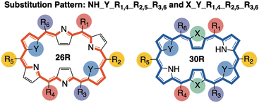
Based on our previous work, we collected a dataset consisting of 562 functionalized hexaphyrins with the X₂Y₂A₂B₂C₂ pattern biased towards high hyperpolarizabilities related to the hyper-Rayleigh scattering β_HRS (Fig. 1).^45,46 More specifically, this dataset contains 242 and 320 meso-substituted and core-modified [26]- and [30]hexaphyrin structures with a Hückel topology (26R and 30R), respectively. All structures contain combinations of the following meso-substituents on the positions R₁–R₆: NO₂, CN, F, H, CH₃, OH and NH₂. Depending on the oxidation state of the hexaphyrin, up to two core-modification sets (X, Y) are present, where NH is replaced by O, S or Se. Only Y modifications were allowed for 26R to avoid charged molecules. The labelling of the 26R and 30R following their substitution pattern is presented in Fig. 1.

Fig. 1 Graphical representation of the [26]- and [30]hexaphyrins with the X₂Y₂A₂B₂C₂ pattern with three pairs of meso-substitution sites {R_1,4; R_2,5; R_3,6} and one or two sets of core-modification sites {X; Y}. For 26R, only Y modifications were allowed.

As already mentioned, this dataset is composed of structures which are skewed towards high nonlinear optical responses since they were generated during NLO contrast optimization runs using an inverse design algorithm. For a detailed comparison between the [26]- and [30]hexaphyrins, we refer to our previous work, in which we extensively described the different design rules for the molecular switches based on these two redox states.⁴⁶ Aside from the target property, the β_HRS response, we computed 35 additional properties. These features can be categorized based on their intrinsic character as indicated in Table 3. By investigating the intercorrelation between the individual 35 features as well as the correlation with our target property, β_HRS, we aim to identify the driving forces responsible for increasing the nonlinear optical response of hexaphyrin macrocycles.

Table 3 Overview of the investigated features in this study grouped in 5 different categories

Category	Features
Aromaticity (structural)	BLA & HOMA
Aromaticity (electronic)	AV1245, AVmin BOA & FLU
Aromaticity (magnetic)	NICS(0), NICSzz(1) & NICS(1)
Orbital	H−1, H, L, L+1, ΔH, ΔL, ΔHL, ΔL_H−1, ΔL+1_H & criteria
Charge transfer	q CT, DCT, Δr & μ01
Electronic	Q trace, μ, IE, EA, ω, η, μe, ΔES1, ΔES2, |Δμ| & DR
Geometrical	Π & ϕp

---

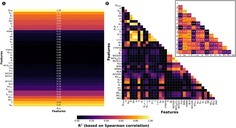
Fig. 2A summarizes the coefficients of determination (R²) based on the Spearman correlation between the 35 features and the β_HRS. Each feature is ranked according to its Spearmann correlation value from a positive to negative correlation. Only 13 of the 35 features have an R² greater than 0.42, namely, Δ_HL, η, ΔE_S1, ΔE_S2, Δ_{L+1_H}, BOA, q_CT, μ, Δ_L, |Δμ|, μ₀₁, Δ_H, and D_CT. These 13 features belong to different categories as defined in Table 3, being either aromaticity-, electronic-, orbital- or charge transfer-based descriptors. Note that even though DR and aromaticity descriptors are commonly used to rationalize the NLO properties, they do not correlate with our target property, with the exception of BOA. A scatterplot of β_HRSversus DR is provided in Fig. S1 (ESI†), which shows that our dataset of hexaphyrins is described by a broad range of DR values ranging from 1.5 until 6.7. Our best-performing structures are distinguished by a DR value close to 5, which is characteristic for a 1D push–pull chromophore. Nevertheless, a large number of structures have a DR around 5, yet a β_HRS below 10 000 a.u. Hence, DR is not able to sufficiently explain the variations in β_HRS. Next, we checked the correlation between the individual 35 features in Fig. 2B. The electronic-based descriptors (IE, EA, ω and μ_e) and the orbital energies of H−1, H, L and L+1 show R² values larger than 0.80, both within their category and between the two categories. Additionally, the geometrical-based descriptors Π and ϕ_p show a high correlation. The last set of features with high R² values are the aromaticity indices based on magnetic criteria, NICS(0), NICS_zz (1) and NICS(1). Intermediate R² values between 0.60 and 0.80 are observed between NICS indices, HOMA and the geometrical descriptors. Overall, the aromaticity indices based on different criteria seem to correlate among each other, where the R² ranges between 0.40 and 0.80.

Fig. 2 Correlation (A) between the β_HRS and 35 features and (B) between the 35 features with a zoom of the intercorrelation between the 10 best-performing features from (A). All correlation plots are based on the Spearman correlation coefficient (R). Each feature is ranked according to its Spearmann correlation value from a positive to negative correlation on the plot on left-hand side.

The additional subplot of Fig. 2B concentrates on the intercorrelation between the 13 features highly correlating with β_HRS. BOA and Δ_{L+1_H} show only low to moderate correlation with respect to the other features. Therefore, these two features may bring unique information into the ML model. Most other properties are characterized by higher R² values. To reduce the number of input features, we opted to remove features that correlate highly with the Δ_HL, since this feature correlates best with the β_HRS response (R² = 0.91). Consequently, the chemical hardness (η) (R² = 0.94), the excitation energy associated to S₂ (ΔE_S2) (R² = 0.82), and Δ_H (R² = 0.77) were not retained. An additional reason for the exclusion of Δ_H is that D_CT and Δ_{L+1_H} also correlate reasonably well with this feature, so the model input of Δ_H may be compensated by these other input features. Despite its significant correlation with four of the remaining input features, we decided to keep D_CT in our input set because of its correlation with β_HRS. In summary, the following properties will be used as input features for the ML model: Δ_HL, Δ_{L+1_H}, BOA, q_CT, μ, Δ_L, μ₀₁, |Δμ|, ΔE_S1, and D_CT.

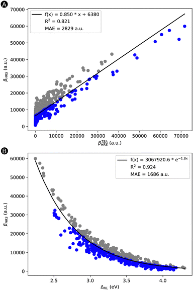
Remark that this list of features still contains the three properties building up the TSA of Oudar and Chemla: |Δμ|, μ₀₁, and ΔE_S1. In Fig. 3A, we plotted our target property β_HRSversus the β^TSA_HRS obtained through Oudar en Chemla's TSA. Despite its frequent successes in other molecular switches, the TSA describes only to a certain degree the target property with an MAE of 2829 a.u. and an R² of 0.821. Interestingly, our best performing feature (Δ_HL) explains already quite well the trend in β_HRS response. We performed an exponential regression on the β_HRSvs. Δ_HL, which resulted in an R² of 0.924 and mean absolute error (MAE) of 1686 a.u. (Fig. 3B). The question arises whether we can better explain the variance of the NLO response, by creating a machine learning (ML) model with additional features that can improve the performance of the TSA and exponential model.

Fig. 3 Scatter plot of the β_HRS response in a.u. versus (A) β^TSA_HRS and (B) the Δ_HL in eV. The regression lines are portrayed by a solid black line and their mathematical expression, R² and MAE are noted in the box above. Data points lying above and below the regression line are colored in blue and grey, respectively.

Training, testing and understanding of machine learning models

Model 1 using ten features. We opted to split our dataset into a separate test (25%) and training set (75%), so that the trained model could also be tested on generalizability. The NLO distribution was kept similar for each set as displayed in Fig. S2 (ESI†). As a result, both sets mainly contain hexaphyrins with a β_HRS below 15 000 a.u. and include a similar number of the best-performing hexaphyrins with a large β_HRS response.

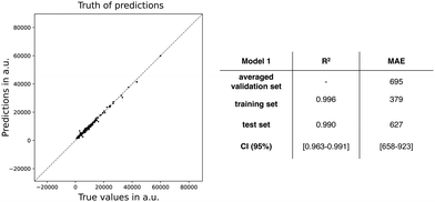
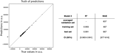
Next, we trained a kernel ridge regression model (KRR) with our selected ten features: Δ_HL, Δ_{L+1_H}, BOA, q_CT, μ, Δ_L, μ₀₁, |Δμ|, ΔE_S1, and D_CT. The objective during the training and hyperparametrization tuning of our ML model was to minimize the MAE. For the hyperparametrization optimization, we used 6-fold cross-validation to prevent overfitting. Using the most optimal hyperparameters, the KRR model was fitted to the full training dataset. Both the averaged cross-validation statistics (MAE and R²), calculated over the six validation sets, and the full training set statistics are reported in Fig. 4, in addition to the external test set statistics along with the 95%-confidence interval (CI). Fig. 4 also includes the truth of predictions plot for the test set data. A markedly lower MAE and higher R² are found for the full training set, which may indicate overfitting during the model training. Regarding the test set, similar values for MAE and R² are obtained as the cross-validation sets (MAE: 695 vs. 627 a.u.) with only a difference of 68 a.u. Compared to the cross-validation, the test set performs a bit better as reflected by the MAE falling out of the 95% confidence interval. In summary, the model generalizes quite well similar unseen data. Remark that the performance of model 1 is significantly better than our exponential model as the model 1's MAE is far below half of the exponential and TSA models.

Fig. 4 Truth of predictions plot: scatter plot of true values (i.e, β_HRS based on quantum chemical calculations) and predictions (β_HRS predicted by model 1) of the test set, together with MAE (in a.u.) and R² for the validation sets (averaged over 6 sets) from the cross-validation, the full training set, and the test set with its confidence interval.

Since some features were found to be somewhat correlated, we performed a feature permutation importance analysis, as implemented into scikit-learn,⁹⁷ to understand how each feature contributes to the performance of our ML model. Here, the feature importances are calculated as the difference between the statistics of the entire dataset and that of the dataset with one feature column permuted. Because the feature permutation has a different interpretation for the test set and training set, we performed this analysis on both sets. All feature permutations are collected in Table 4 for the MAE statistics.

Table 4 Feature permutation importance of model 1 with the differences in statistics between the actual dataset together with the permuted datasets and their standard deviations

	ΔMAE (train)	ΔMAE (test)
Δ HL	1653 ± 73	1559 ± 113
D CT	3789 ± 139	3650 ± 193
Δ L+1_H	1430 ± 58	1123 ± 86
Δ L	1429 ± 69	1347 ± 129
μ 01	2321 ± 99	2021 ± 182
q CT	2439 ± 102	1874 ± 184
ΔES1	2496 ± 186	2130 ± 251
|Δμ|	1141 ± 79	854 ± 118
BOA	1260 ± 71	1007 ± 122
μ	983 ± 97	1179 ± 57

---

By inspecting the importances of the test set, we can derive which features will contribute to the generalization power of our model. Additionally, the feature importances related to the training set can identify which features are possibly overfitting our trained model. At first glance, both test and training set of model 1 present similar trends for their feature importances and generally within the same order of magnitude. Consequently, the interpretation of this analysis for both datasets is the same. The D_CT is the most influential feature in the model, both for the training and test set of model 1 with a potential increase in MAE value of around 3700 a.u. Other important features are: ΔE_S1, q_CT, and μ₀₁. Unexpectedly, Δ_HL comes in fourth place despite its high correlation with the target property. A slight discrepancy in feature importances between the train and test set is observed for ΔE_S1, μ₀₁, and especially q_CT. Since this divergence might indicate that model 1 is overfit, a reduction of input features is advisable. Our strategy is to continue reducing the feature set based on the balance between model performance and feature importances. The analysis of this strategy is described in ESI† (cf. Fig. S3). By consecutively removing the feature with the lowest feature importance, new models are generated until the resulting model has a (too) negative effect on the model performance, here through the MAE statistic. In the end, we obtain our final model, denoted as model 2, with only six features: Δ_HL, q_CT, Δ_L, μ₀₁, ΔE_S1, and D_CT. Note that this final model still contains the features of the TSA and the exponential models, except for |Δμ|.

Model 2 using 6 features. Based on the previous analysis, we trained a new KRR model, called model 2, consisting of three charge-transfer based features (q_CT, μ₀₁, and D_CT), two orbital based features (Δ_HL and Δ_L), and one electronic feature (ΔE_S1). Similarly, we focused on minimizing the MAE of the ML model. Fig. 5 summarizes the most important statistics for the validation sets from the 6-fold cross-validation hyperparameter optimization, the full training set, and the test set. The R² and MAE values of model 2 are slightly worse than our previous model, for which the MAE of the test set increases by merely 40 a.u. This 6% augmentation is acceptable given the 40% reduction in feature size. As observed in model 1, a small difference in MAE between the cross-validation data and the test set is observed. In contrast to model 1, both statistics of the test set fall within the 95% confidence interval.

Fig. 5 Truth of predictions plot: scatter plot of true values (i.e, β_HRS based on quantum chemical calculations) and predictions (β_HRS predicted by model 2) of the test set, together with MAE (in a.u.) and R² for the validation sets (averaged over 6 sets) from the cross-validation, the full training set, and the test set with its confidence interval.

Next, we applied the feature permutation importance analysis on model 2 (Table 5). In contrast to the model 1, Δ_HL becomes equally important as D_CT for both the training and test sets, whereas μ₀₁ and Δ_L increase substantially in feature importance. Note the slight discrepancy between training and test set for q_CT in terms of MAE. In conclusion, all features significantly contribute to the model performance, both for the training and test data.

Table 5 Feature permutation importance of model 2 with the differences in statistics between the actual dataset together with the permuted datasets and their standard deviations

Model 6 features	ΔMAE (train)	ΔMAE (test)
Δ HL	4735 ± 186	4347 ± 295
D CT	4730 ± 214	4498 ± 360
Δ L	1247 ± 72	1043 ± 106
μ 01	2982 ± 154	2898 ± 267
q CT	2152 ± 133	1776 ± 243
ΔES1	2028 ± 90	1960 ± 195

---

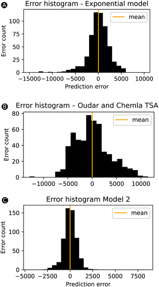
Despite the slight drop in performance going from model 1 to model 2, the performance of model 2 remains significantly better than our initial exponential model based on only one feature Δ_HL. Fig. 6 compares three error-bar histograms showing the prediction error distributions for the exponential model, the two-state model of Oudar and Chemla, and model 2. For the construction of the error-bar plots, all datapoints were considered. Besides a much narrower distribution for model 2, we also note that the exponential model and the two-state model description of this total dataset results in a significant number of datapoints having errors above 2000 or below −2000 a.u., being 166 or 30% for the exponential model and and 314 or 56% for the TSA, while model 2 has as few as 9 datapoints within this range. In short, the addition of other features besides the Δ_HL allows model 2 to drastically reduce the number of outliers. To confirm this observation, we computed the MAE of these 166 systems based on the model 2 predictions, and, indeed, the initial MAE of 3580 a.u. using the exponential model is significantly reduced to 587 a.u. by using model 2.

Fig. 6 Error bars for the prediction of the β_HRS in a.u. for the exponential model (A), TSA model (B) and model 2 (C) using the complete dataset (training & test sets).

Analysis of the machine learning model 2 with SHAP. The question still remains how these additional features aided in the prediction of the NLO response. To further elucidate the influence of the features on the β_HRS response, we select model 2 as our main model of interest. We employed the SHAP Python package^99,100 and its version in R for dependent features,¹⁰¹ which contains techniques to explain black-box machine learning models. Using this analysis, we aim to understand our model's predictions based on the features on which the model is built. We considered the full dataset for the SHAP analysis discussion, but a similar analysis for the test set is provided in the ESI† (Fig. S4). To summarize the average impact of each feature on the model output, we present a bar plot in Fig. 7A. 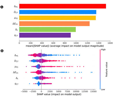This average impact is calculated with respect to the so-called baseline value, which in our case is the average of all predicted β_HRS values, being 10 500 a.u. The trends of Fig. 7 are the same regardless of the dataset type. All features have a nonnegligible impact on the magnitude of the model output, with a minimal average contribution of 900 a.u. Our most impactful features are the Δ_HL, D_CT and μ₀₁, with mean SHAP values over 1200 a.u., which are well above the MAE.

Fig. 7 SHAP analysis of model 2. (A) Bar plot containing the mean absolute SHAP value for each feature over all samples. (B) Beeswarm plot with SHAP values of all data points while highlighting the feature value.

To gain insight on how each feature impacts the model predictions (SHAP value) depending on the feature value, we provide a beeswarm plot in Fig. 7B. Both Δ_HL and ΔE_S1 show the same trend where lower feature values have a positive impact on the NLO response, while high feature values have a negative impact on the output. That means that the lower is the HOMO and LUMO energy gap or the excitation energy, the higher is the β_HRS response. On the other hand, D_CT, μ₀₁, and Δ_L behave in the opposite manner, where higher and lower values have a positive and negative impact on the β_HRS response, respectively. With respect to the baseline (SHAP values of 0), most structures have lower SHAP values, but they do not extend that much when compared to the higher SHAP values (SHAP ranges are between −4000 and 16 000 a.u.). There is no clear trend for q_CT, for which we see an overlap between high and low q_CT to the left and the right of the baseline. Additional information on the exact relationship between the feature value and SHAP value is provided in Fig. S5A–F in the ESI.† Here, we observe a reversed and sharp v-curve relationship between q_CT and its SHAP value. This v-curve peaks around a feature value of 0.8. Values lower and higher than 0.8 almost linearly decrease in SHAP contribution. The SHAP values associated with q_CT generally contribute less but quite evenly with respect to the baseline. Hence, our main features contributing most to the prediction of high NLO responses by model 2 are primarily orbital and charge transfer-based features, Δ_HL and D_CT as well as μ₀₁. Note that the relationship between the HOMO–LUMO energy difference and its SHAP contribution to β_HRS seems close to exponential (Fig. S5A in ESI†), as we observed before for the exponential regression model.

Difference between 26R and 30R. As mentioned before, our dataset consists of hexaphyrin structures with the same rectangular Hückel topology but two different oxidation states: [26]- and [30]hexaphyrins, denoted as 26R and 30R, respectively. During our previous studies,^45,46 we discovered that higher NLO responses can be obtained for 26R compared to 30R. On top of that, the preference for the type and position of the functionalizations to increase the NLO response are different depending on the oxidation state. In this work, we aim to gain a better understanding on which driving forces can be related to these differences in NLO response between the 26R and 30R, and thus also the differences in their optimal substitution patterns. First, we will compare the performance of the ML model for the 26R and 30R hexaphyrins and, second, we will determine which features have the strongest impact on the prediction of their respective NLO responses.

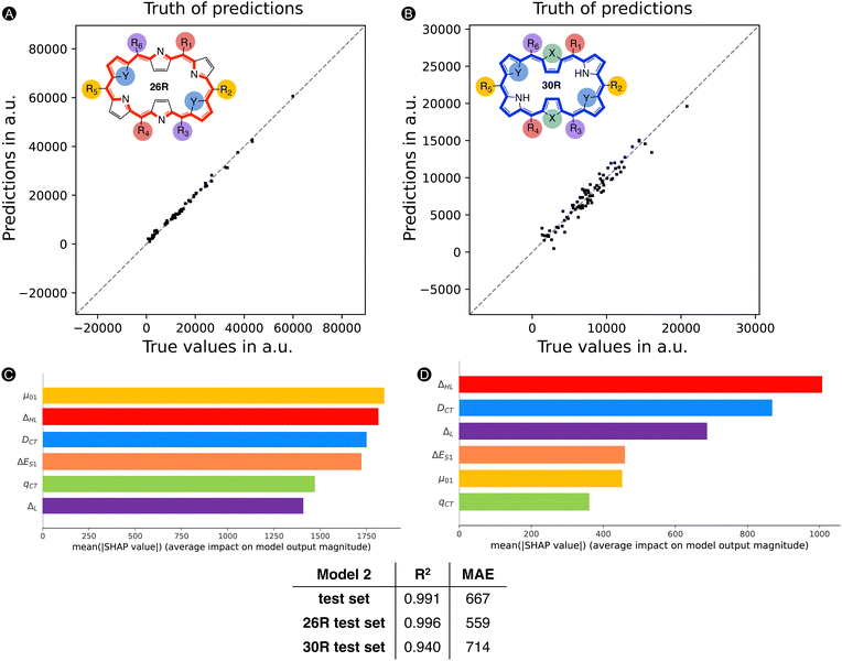
First, we reassessed the MAE for the [26]- and [30]hexaphyrin systems separately by focusing only on those present in the test set. Fig. 8 summarizes the scatterplots of the true values versus the predictions by ML model 2 for the subsets of [26]- and [30]hexaphyrins. The MAEs of the test sets containing either 26R or 30R systems remain around the same value as for the total test set. In addition, both subsets show an R² of 0.94 and more, with the model performance being a bit better for the 26R systems.

Fig. 8 Truth of predictions plot: scatter plot of true values (i.e., β_HRS based on quantum chemical calculations) and predictions (β_HRS predicted by model 2) with MAE and R² for (A) the [26]hexaphyrins and (B) [30]hexaphyrins present in the test set. In addition, SHAP analysis of model 2. Bar plot containing the global feature importances as the mean absolute SHAP value for each feature for the (C) 26R and (D) 30R subsets of the entire dataset.

Next, we reapplied the SHAP analysis to the 26R and 30R hexaphyrin subsets (both training and test sets) to verify if the features contribute differently to the prediction of their NLO response. In Fig. 8, two barplots are displayed highlighting the average impact on the model output for all [26]- (left) and [30]hexaphyrins (right), relative to their respective baseline, 14 163 a.u. for the former and 7731 a.u. for the latter. Despite the base value being adjusted for each subset, we clearly observe that the average SHAP values are lower for 30R systems than 26R macrocycles for the different features. Importantly, the top three features influencing the average impact on the model output differ for the two hexaphyrin redox states. The [26]hexaphyrins are mostly impacted by the μ₀₁, Δ_HL, and D_CT, in nearly equal amounts. In fact, all features still significantly contribute to the prediction with a SHAP value of minimally 1400 a.u. Regarding the 30R systems, Δ_HL becomes more important and μ₀₁ drops significantly in β_HRS contribution. D_CT remains in the top 3 of dominant features. Interestingly, Δ_L now becomes a vital feature in terms of the average contribution to the output prediction. The S₁ excitation energy remains on the fourth place but seems less influential than for the 26R. For both hexaphyrins, q_CT is one of the least impactful features on the model output. Note that for the [30]-hexaphyrins ΔE_S1, μ₀₁ and q_CT contribute, on average, a relatively small amount.

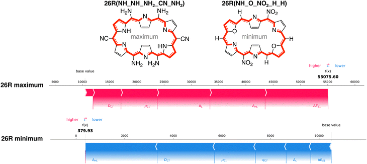
How do the features influence our best- and worst-performing 26R and 30R in terms of NLO response? Our best-performing 26R are denoted as 26R(NH_NH_NH₂_CN_NH₂), 26R(NH_Se_NH₂_CN_NH₂) and 26R(NH_S_NH₂_CN_NH₂) and all contain the same meso-substitution pattern with 2 sets of strongly electron-donating groups (EDGs) and 1 set of strongly electron-withdrawing groups (EWGs). The three 26R macrocycles with the lowest NLO response (26R(NH_O_NO₂_H_H), 26R(NH_S_CN_CN_CN) and 26R(NH_S_NO₂_CN_CN)) consist of combinations of core-modifications and meso-substitutions with 1 or 3 pairs of EWGs. In Fig. 9, we present the force plots¹⁰⁰ of the 26R systems with minimal and maximal β_HRS response, with the baseline at 10 500 a.u. taken as the prediction average of the full dataset (including both [26]- and [30]hexaphyrins). These force plots depict for each instance the influence of each feature on the model's prediction. Starting from the base value, each feature increases (red) or decreases (blue) the base value to obtain the function value (f(x)). The other force plots of the second and third structures with either minimal and maximal β_HRS responses can be found in the ESI† (Fig. S6–S9).

Fig. 9 Force plot of the 26R system with the highest and lowest β_HRS response corresponding to 26R(NH_NH_NH₂_CN_NH₂) and 26R(NH_O_NO₂_H_H), respectively. Features highlighted in red positively contribute with respect to the base value, while those highlighted in blue lower the NLO response prediction.

All force plots of best performing 26R structures show that all six features have a positive impact on the model's prediction. Hence, all features aid in increasing the base value towards the predicted value. ΔE_S1 has the most influence for the three maxima. Depending on the optimum, either μ₀₁, Δ_HL, and Δ_L play an important role. Interestingly, D_CT plays a minor role, despite being in the top three of average feature impact on model output magnitude (Fig. 8A). The opposite trend is observed for the 26R systems with a low β_HRS response, where all features lower the base value. Here, D_CT and Δ_HL are the most important features. Therefore, D_CT has a larger impact in reducing the NLO response than enhancing it, relative to the other features.

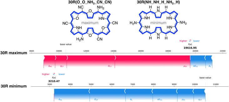
The best-performing 30R systems contain two sets of core-modifications and EWGs and one set of EDGs, 30R(O_O_NH₂_CN_CN), 30R(O_S_NH₂_CN_CN) and 30R(O_O_NH₂_NO₂_CN). Our worst-performing are 30R(NH_NH_H_NH₂_H), 30R(NH_NH_H_OH_H) and 30R(NH_NH_H_F_H) and only consist of one set of strong EDGs or weak EWGs as meso-substituents on the macrocycle and no core-modifications. Similarly to the 26R systems, we only display the systems with the lowest and highest β_HRS response in Fig. 10.

Fig. 10 Force plot of the 30R system with the highest and lowest β_HRS response corresponding to 30R(O_O_NH₂_CN_CN) and 30R(NH_NH_H_NH₂_H), respectively. Features highlighted in red positively contribute with respect to the base value, while those highlighted in blue lower the NLO response prediction.

In contrast to the best 26R, the force plots of the best 30R structures show that not all features necessarily increase the baseline prediction. In all three structures, ΔE_S1 has the highest negative impact on the predicted average. Surprisingly, even though μ₀₁ is ranked second to lowest for the [30]hexaphyrins, it shows the highest positive impact for the 30R maximum followed by D_CT. In the two remaining structures, other features such as q_CT, D_CT, and Δ_HL play a varying positive role on the NLO response. In contrast, the worst performing 30R structures behave similarly to the worst performing 26R with D_CT, Δ_HL, and to a lesser degree Δ_L as the main important features. This explains the gain in importance of D_CT for 30R compared to 26R, as this feature greatly impacts both high and low responses for the former but only low responses for the latter.

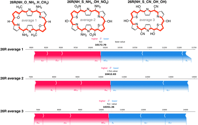
Aside from the structures with the highest and lowest β_HRS response, we selected three additional systems with predicted β_HRS values close to the average of the entire dataset, the baseline of our SHAP analysis. We focused on 26R structures, as we found for both high and low response structures similar dominant features. These [26]hexaphyrins incorporate at least one set of core-modifications and different combinations of meso-substitutions on their macrocycle: 26R(NH_O_NH₂_H_CH₃), 26R(NH_S_NH₂_OH_NO₂) and 26R(NH_S_CN_CN_OH). The force plots of these systems are provided in Fig. 11.

Fig. 11 Force plot of 26R(NH_O_NH₂_H_CH₃), 26R(NH_S_NH₂_OH_NO₂), and 26R(NH_S_CN_CN_OH). Features highlighted in red increase the NLO response with respect to the base value, while those highlighted in blue lower the NLO response.

For all three systems, we observe that nearly all individual features distinctly contribute to the predicted NLO response, some positively and some negatively. A clear trend on how each feature influences the final prediction of the model is difficult to establish. Despite the similar total prediction output, a different combination of features is responsible for the predicted β_HRS value. For example, for 26R average 2, the two orbital and one electronic-based features increase the response prediction, whereas the charge-transfer-based features diminish the prediction by the same amount. The similarly substituted 26R average 3, having the same core-modification set and also two sets of EDGs and one set of EWGs (though on different positions), differs with the previous structure in that μ_0,1 now positively contributes and Δ_L negatively.

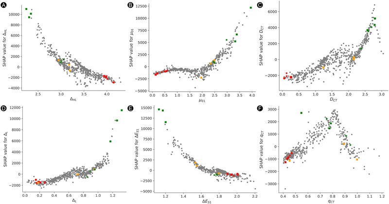
Lastly, to estimate where these 15 selected systems are positioned within the SHAP versus feature value space, we plotted dependency plots for each feature. The dependency plots in Fig. 12 show the SHAP value of a feature versus the feature value. The 26R and 30R systems are represented by a square and star marker, respectively. The systems are colored in red, orange and green corresponding to lowest, medium and highest responses accordingly. The scatter plot for Δ_HL as presented in Fig. 12A shows that the best-performing 26R have high SHAP values for low Δ_HL feature values. The β_HRS response of the orange markers and the best-performing 30R, represented by green stars, are only slightly positively influenced by the Δ_HL except for one system 26R(NH_O_NH₂_H_CH₃) with an average β_HRS response. For example, the SHAP value for Δ_HL of 26R(NH_NH_NH₂_CN_NH₂) is much higher and positive, 11 019 a.u., than the best-performing 30R with a SHAP value of 836 a.u. For the worst performing structures depicted in red, the Δ_HL has always a negative influence on the model output. Fig. 12B–D show the opposite of Fig. 12A, where high feature values have a positive impact on the model's output and low values the opposite. Nonetheless, a few outliers should be noted which deviate from the expected trend. Regarding the μ₀₁ feature (Fig. 12B), the best-performing [30]hexaphyrin-based structures are close to the [26]hexaphyrins with an average β_HRS response, except for one system, 30R(O_O_NH₂_CN_CN), which has a higher μ₀₁ than the other [30]hexaphyrins. In addition, one 26R system, 26R(NH_S_NH₂_OH_NO₂), is negatively impacted by μ₀₁ as reflected by its negative SHAP value and lower feature value. The opposite is observed for D_CT (Fig. 12C), where the best-performing [30]hexaphyrin-based structures lie closely to the best-performing [26]hexaphyrin-based structures, with the exception of 30R(O_S_NH₂_CN_CN), which resides near the average performing structures. For those two charge-transfer-based descriptors, the worst-performing 26R and 30R are all at the end of the curves. The average-response structures are more spread for D_CT. In Fig. 12D, one of the average 26R structures, 26R(NH_S_CN_OH_OH), is positioned closer to those with a low β_HRS response highlighted in red, because lower differences between L and L+1 (Δ_L) result in more negative SHAP values. Fig. 12E shows similar trends as Fig. 12A, where the best-performing 26R structures show positive SHAP values for low feature values and the opposite is true for the worst 26R and 30R structures. Except for 26R(NH_O_NH₂_H_CH₃), all average-structures are characterized by a postive SHAP value with an excitation energy ΔE_S1 around 1.6 eV. In contrast to Δ_HL, the best-performing 30R structures are much closer to the overall worst performing structures and are characterized by negative SHAP and low ΔE_S1 values. The outlying 26R(NH_O_NH₂_H_CH₃) is also positioned closer to the best-performing 30R structures. Finally, a general trend remains difficult to distinguish for the q_CT feature in Fig. 12F. As mentioned before, the peak of the structures with the highest positive impact on the model is perceived at a feature value of 0.8. Remarkably, our best-performing structure 26R(NH_NH_NH₂_CN_NH₂) has a very high positive impact on the final prediction for a low feature value of 0.57 but lies well outside the v-curve.

Fig. 12 Dependency plots highlighting the feature SHAP versus the feature value for (A) Δ_HL, (B) μ₀₁, (C) D_CT, (D) Δ_L, (E) ΔE_S1 and (F) q_CT. The 26R and 30R systems are represented by a square and star marker, respectively. The 15 systems are colored in red, orange and green corresponding to lowest, medium and highest β_HRS responses accordingly.

External test sets: new meso-substitution pattern and different conformers. Now that we gained insight into how the features influence the [26]- and [30]hexaphyrins, our next goal is to investigate whether our ML model can generalize other hexaphyrin macrocycles. As our dataset only consisted of hexaphyrin structures with the A₂B₂C₂meso-substitution pattern, can our model describe other substitution patterns or even other types of hexaphyrins with different topologies? To test this, we constructed three additional test sets with new categories of hexaphyrins investigated in our previous works (structures are shown in Fig. 13).^44,46,102 A first test set, called 26R(A₂BC₂D), contains 49 [26]hexaphyrins with a different substitution pattern A₂BC₂D. A second set of 8 [26] and 10 [28]hexaphyrins having the dumbell (26D) and Möbius topology (28M), respectively, and the same A₂B₂C₂ substitution pattern is collected in test set, 26D(A₂B₂C₂) + 28M(A₂B₂C₂). Lastly, a third test set 28R(A₂BC₂D) contains 39 [28]hexaphyrins with the rectangular topology (28R) and the A₂BC₂D substitution pattern. This last substitution pattern was selected for the 28R system, because our initial A₂B₂C₂meso-substitution pattern allows the 28R to become centrosymmetric with a zero-valued β_HRS response per definition.

Fig. 13 Scatter plot of the β_HRS response (in a.u.) versus the Δ_HL (in eV) for (A) 26R(A₂BC₂D), (B) 26D(A₂B₂C₂) + 28M(A₂B₂C₂), (C) 28R(A₂BC₂D). The exponential regression line is portrayed by a solid black line and its mathematical expression is given in the box. Data points from the initial dataset are highlighted in grey, but each new test set is coloured in red, salmon, orange and green for 26R(A₂BC₂D), 26D(A₂B₂C₂), 28M(A₂B₂C₂) and 28R(A₂BC₂D), respectively.

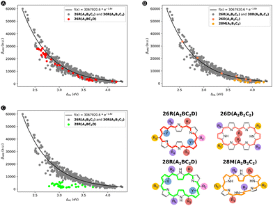
To start off, we replotted in Fig. 13 the relationship between the β_HRSversus Δ_HL for our initial dataset, in which we additionally highlighted one of the extra test sets in a different color. The two test sets (26R(A₂BC₂D) and 26D + 28M(A₂B₂C₂)) presented in Fig. 13A and B, respectively, follow the trend, thus associating high β_HRS responses with low Δ_HL values. However, the test set containing 28R(A₂BC₂D) structures does not follow this exponential relationship. In essence, systems with either a different substitution pattern or different hexaphyrin conformations can behave similarly to the 26R(A₂B₂C₂) and 30R(A₂B₂C₂) dataset. In the ESI,† we also provided the scatterplots regarding TSA (i.e., β_HRSversus β^TSA_HRS) for our external test sets. The 26R(A₂BC₂D) dataset but also 28R(A₂BC₂D) (reasonably) follow the previous TSA trend, while 26D + 28M(A₂B₂C₂) is not well described by this model.

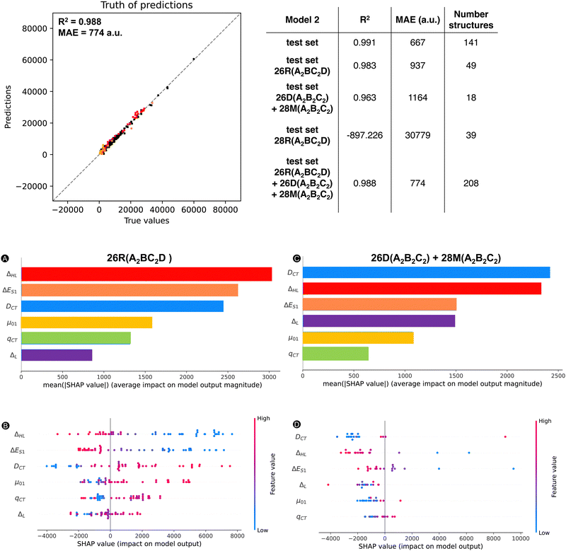
Subsequently, we predicted the β_HRS response of the three test sets with our ML model 2. For the individual scatter plots for each new test set, we refer to the ESI† (Fig. S11). If we combine our initial test set with the two test sets 26R(A₂BC₂D) and 26D + 28M(A₂B₂C₂), for which the exponential model provided a good description, and recalculate the MAE and R², Fig. 14 is obtained. Here, 26R(A₂BC₂D) and 26D(A₂B₂C₂) + 28M(A₂B₂C₂) are colored in red and salmon and orange, respectively. Even after the addition of the new data points, our R² of 0.988 stays similar to that of the initial test set (R²: 0.991). Since our ML model has not yet encountered these types of structures, the MAE increases but not substantially (774 a.u. vs. 667 a.u.). This observation also applies to the R² of the first and second extra test set individually in comparison to the initial test set (Fig. 14). However, the MAEs of the individual (26R(A₂BC₂D) and 26D + 28M(A₂B₂C₂)) sets increase by 40% and 75%, respectively, so a different substitution pattern is generalized better than a change of topology and/or oxidation state. Nonetheless, these predictions are still better than the initial exponential model (MAE of 1686 a.u.) and the revised exponential model, including these first two external test sets (MAE of 1736 a.u. and R² of 0.913). As expected, the 28R(A₂BC₂D) test set performs the worst of all new sets with an MAE almost 20 times higher than our exponential model. This bad performance stems from the negative β_HRS response predictions by model 2 for the 28R(A₂BC₂D) test sets. In summary, our ML model is able to reasonably describe hexaphyrins of the same oxidation state and topology with a different substitution pattern and hexaphyrins of different oxidation state and topology, with the exception of the 28R structures.

Fig. 14 Truth of predictions plot: scatter plot of true values (i.e, β_HRS based on quantum chemical calculations) and predictions (β_HRS predicted by model 2) on the initial test set, and new test sets 26R(A₂BC₂D) and 26D + 28M(A₂B₂C₂) with MAE and R² for the initial test set, the three extra test sets, and the total test set excluding the 28R (figure statistics). Below, SHAP analysis of the first two external test sets. (A) Bar plot containing the feature importances as the mean absolute SHAP value for each feature and all samples for 26R(A₂BC₂D) (B) bar plot containing the feature importances as the mean absolute SHAP value for each feature and all samples for 26D + 28M(A₂B₂C₂) (C) beeswarm plot with SHAP values of all data points while highlighting the feature value for 26R(A₂BC₂D). (D) Beeswarm plot with SHAP values of all data points while highlighting the feature value for 26D + 28M(A₂B₂C₂).

To gain insight into which features contribute to the prediction for the first two external test sets, we applied our SHAP analysis tools (using the average prediction of the original total dataset as base value) to understand our model's decisions (Fig. 14). For the 26R(A₂BC₂D) set, which contains [26]hexaphyrins with a different substitution pattern, the Δ_HL is the most significant feature (Fig. 14A). This feature rises from second to first place in importance compared to the 26R conformers having A₂B₂C₂ pattern in Fig. 8A. The second most influential feature of this external dataset is ΔE_S1, which has also increased in importance. Surprisingly, our top feature for the initial 26R dataset, μ₀₁, drops significantly in averaged SHAP value. D_CT remains in the third position and q_CT and Δ_L are still the least influential features. Apart from the feature importance, the trends in Fig. 14B are overall quite similar as in Fig. 7B, which deals with the entire dataset and does not distinguish between the different hexaphyrin types. Higher values for D_CT, μ₀₁ and Δ_L correspond with positive impacts on the model output. The opposite is still true for Δ_HL and ΔE_S1. For our second test set, 26D + 28M(A₂B₂C₂), D_CT and Δ_HL are our most important features (Fig. 14C), which is more or less in line with the [30]hexaphyrins in Fig. 8B. Δ_L and ΔE_S1 become equally important and the latter jumps to the third place in the ranking compared to the trends observed for the 30R hexaphyrins. Again, q_CT is among the worst-performing of all features. Since only 18 data points are present in this external test set, the beeswarm plot in Fig. 14D becomes less interpretable but it shows similar trends as Fig. 7B for the entire dataset. Except for some small deviations in the Δ_L feature vs. SHAP scatter plot in Fig. S12D in the ESI,† the other scatter plots (Fig. S12, ESI†) confirm that the two external datasets follow indeed the general trend.

Conclusion

In this work, we employed explainable machine learning to further understand the underlying factors influencing the NLO response of chemically functionalizated [26]- and [30]hexaphyrins. To this end, we investigated various quantum-chemical descriptors and their relationship with our target property, β_HRS. Only 13 features correlated sufficiently with R² values above 0.4. They can be categorized as, primarily, orbital-based (4) and charge-transfer (3) features but also electronic (5) and aromaticity (1) descriptors. The intercorrelation between each of these thirteen features was also established. Before applying any machine-learning model to our dataset, we checked two additional models to predict the β_HRS response based on either the two-state approximation of Oudar and Chemla and only the HOMO–LUMO energy gap. Overall, the HOMO–LUMO gap is the best-performing feature in predicting the β_HRS response of the hexaphyrin macrocycles for which exponential regression yielded an MAE of 1686 a.u. After removing highly intercorrelating features, we constructed a ML model using 6-fold cross-validated kernel ridge regression with 10 input features and the MAE as the validation metric (model 1). As model 1 shows signs of overfitting, we further reduced the number of features to 6 by keeping the balance between the model performance and high feature importances for the model. Our final ML model contained 6 features only including orbital, electronic and charge-transfer based descriptors and resulted in an MAE value far below half of that of the exponential model. We applied explainable ML model techniques such as a SHAP analysis to obtain the average impact of each feature on the model output. From the SHAP analysis, we concluded that all of the features have an impact on the model output, but Δ_HL, D_CT, and μ₀₁ influence the model output the most. We would like to emphasize that even though nearly all features of the TSA and the exponential model are included in the ML input feature set, other descriptors such as D_CT still have a big importance on both the performance of the model as the interpretation of the final predictions. Next, we re-evaluated the performance of our model for the two subgroups in our dataset, the 26R and 30R structures. By reapplying the SHAP analysis on the 26R and 30R structures separately, we could scrutinize whether the most influential features are different for each group. We found that, besides μ₀₁, the NLO response of the 26R structures are mostly affected by Δ_HL and D_CT. For the 30R, D_CT gains importance whereas that of μ₀₁ significantly drops. Analysis of the three best- and worst-performing 26R and 30R structures indicated that, even though the D_CT is in the top three of important features, the best-performing 26R structures are less influenced by this property in contrast to 30R. Lastly, we assessed the generalization of our ML model by predicting the NLO response of other types of hexaphyrins, which were not present in the training dataset. Three external datasets were constructed with either 26R or 28R with another meso-substitution pattern, and a collection of hexaphyrins sharing the original meso-substitution pattern but with another topology (26D and 28M). With the exception of the 28R set, our model could reasonably describe our additional external test sets. Our SHAP analysis concluded that 26R(A₂BC₂D) resembles the 26R(A₂B₂C₂) set, except for μ₀₁, and that the 26D + 28M(A₂B₂C₂) set follows the trends of the 30R.

Author contributions

E. D., F. D. V., and M. A. conceptualized the project. E. D. performed all quantum chemical calculations, coded and constructed the ML models based on the code provided by M. J. In addition, M. J. supported E. D. in case of technical difficulties with the code. F. D. V. supervised the project. E. D. analyzed the data. The first draft of the manuscript was written by E. D. and F. D. V. All authors were involved in future editing and reviewing process. All authors have read and agreed to the published version of the manuscript.

Data availability

The data supporting this article have been included as part of the ESI.†

Conflicts of interest

There are no conflicts of interest to report.

Acknowledgements

F. D. V. and M. A. wish to thank the VUB for the Strategic Research Program awarded to the ALGC research group. E. D. thanks the Fund for Scientific Research-Flanders (FWO-11E0321N) for financial support. The resources and services used in this work were provided by the VSC (Flemish Supercomputer Center), funded by the Research Foundation – Flanders (FWO) and the Flemish Government. E. D. and F. D. V. would like to thank Prof. Dr Marc Elskens at the Vrije Universiteit Brussel and MSc Mark Heezen for the fruitful discussions on the topic of machine-learning models and statistics.

Notes and references

1. P. A. Franken, A. E. Hill, C. W. Peters and G. Weinreich, Phys. Rev. Lett., 1961, 7, 118–119.
2. T. Kaino and S. Tomaru, Adv. Mater., 1993, 5, 172–178.
3. B. J. Coe, Chem. – Eur. J., 1999, 5, 2464–2471.
4. S. R. Marder, Chem. Commun., 2006, 131–134.
5. J. A. Delaire and K. Nakatani, Chem. Rev., 2000, 100, 1817–1846.
6. J. L. Zhang, J. Q. Zhong, J. D. Lin, W. P. Hu, K. Wu, G. Q. Xu, A. T. S. Wee and W. Chen, Chem. Soc. Rev., 2015, 44, 2998–3022.
7. L. Sun, Y. A. Diaz-Fernandez, T. A. Gschneidtner, F. Westerlund, S. Lara-Avila and K. Moth-Poulsen, Chem. Soc. Rev., 2014, 43, 7378–7411.
8. S. Gao, X. Yi, J. Shang, G. Liu and R.-W. Li, Chem. Soc. Rev., 2019, 48, 1531–1565.
9. F. Castet, V. Rodriguez, J.-L. Pozzo, L. Ducasse, A. Plaquet and B. Champagne, Acc. Chem. Res., 2013, 46, 2656–2665.
10. F. Meyers, S. R. Marder, B. M. Pierce and J. L. Bredas, J. Am. Chem. Soc., 1994, 116, 10703–10714.
11. S. R. Marder, C. B. Gorman, F. Meyers, J. W. Perry, G. Bourhill, J.-L. Bredas and B. M. Pierce, Science, 1994, 265, 632–635.
12. J. M. Hales, S. Barlow, H. Kim, S. Mukhopadhyay, J.-L. Brédas, J. W. Perry and S. R. Marder, Chem. Mater., 2014, 26, 549–560.
13. V. Postils, Z. Burešová, D. Casanova, B. Champagne, F. Bureš, V. Rodriguez and F. Castet, Phys. Chem. Chem. Phys., 2024, 26, 1709–1721.
14. P. Beaujean, L. Sanguinet, V. Rodriguez, F. Castet and B. Champagne, Molecules, 2022, 27, 2770.
15. A. Plaquet, M. Guillaume, B. Champagne, F. Castet, L. Ducasse, J.-L. Pozzo and V. Rodriguez, Phys. Chem. Chem. Phys., 2008, 10, 6223–6232.
16. P. K. Samanta and R. Misra, J. Appl. Phys., 2023, 133, 020901.
17. P. Beaujean and B. Champagne, Inorg. Chem., 2022, 61, 1928–1940.
18. Y. Yao, H.-L. Xu and Z.-M. Su, J. Mater. Chem. C, 2022, 10, 12338–12349.
19. C. Naim, F. Castet and E. Matito, Phys. Chem. Chem. Phys., 2021, 23, 21227–21239.
20. J. L. Oudar and D. S. Chemla, J. Phys. Chem., 1977, 66, 2664–2668.
21. L. Lescos, S. P. Sitkiewicz, P. Beaujean, M. Blanchard-Desce, B. Champagne, E. Matito and F. Castet, Phys. Chem. Chem. Phys., 2020, 22, 16579–16594.
22. C. Tonnelé and F. Castet, Photochem. Photobiol. Sci., 2019, 18, 2759–2765.
23. C. Tonnelé, B. Champagne, L. Muccioli and F. Castet, Phys. Chem. Chem. Phys., 2018, 20, 27658–27667.
24. Y. Zhang and B. Champagne, J. Phys. Chem. C, 2013, 117, 1833–1848.
25. F. Bondu, J. Quertinmont, V. Rodriguez, J.-L. Pozzo, A. Plaquet, B. Champagne and F. Castet, Chem. – Eur. J., 2015, 21, 18749–18757.
26. M. Pauley and C. Wang, Rev. Sci. Instrum., 1999, 70, 1277–1284.
27. A. E. Stiegman, E. Graham, K. J. Perry, L. R. Khundkar, L. T. Cheng and J. W. Perry, J. Am. Chem. Soc., 1991, 113, 7658–7666.
28. C. Dehu, F. Meyers and J. L. Bredas, J. Am. Chem. Soc., 1993, 115, 6198–6206.
29. T. Tanaka and A. Osuka, Chem. Rev., 2017, 117, 2584–2640.
30. H. Mori, T. Tanaka and A. Osuka, J. Mater. Chem. C, 2013, 1, 2500–2519.
31. S. Pascal, S. David, C. Andraud and O. Maury, Chem. Soc. Rev., 2021, 50, 6613–6658.
32. K. Shimomura, H. Kai, Y. Nakamura, Y. Hong, S. Mori, K. Miki, K. Ohe, Y. Notsuka, Y. Yamaoka and M. Ishida, et al. , J. Am. Chem. Soc., 2020, 142, 4429–4437.
33. Y. Ding, W.-H. Zhu and Y. Xie, Chem. Rev., 2017, 117, 2203–2256.
34. T. Woller, P. Geerlings, F. De Proft, B. Champagne and M. Alonso, Molecules, 2018, 23, 1333.
35. T. Woller, P. Geerlings, F. De Proft, B. Champagne and M. Alonso, J. Phys. Chem. C, 2019, 123, 7318–7335.
36. M. Torrent-Sucarrat, S. Navarro, E. Marcos, J. M. Anglada and J. M. Luis, J. Phys. Chem. C, 2017, 121, 19348–19357.
37. J. M. Lim, Z. S. Yoon, J.-Y. Shin, K. S. Kim, M.-C. Yoon and D. Kim, Chem. Commun., 2008, 261–273.
38. Z. S. Yoon, J. H. Kwon, M.-C. Yoon, M. K. Koh, S. B. Noh, J. L. Sessler, J. T. Lee, D. Seidel, A. Aguilar, S. Shimizu, M. Suzuki, A. Osuka and D. Kim, J. Am. Chem. Soc., 2006, 128, 14128–14134.
39. Z. S. Yoon, D.-G. Cho, K. S. Kim, J. L. Sessler and D. Kim, J. Am. Chem. Soc., 2008, 130, 6930–6931.
40. T. K. Ahn, J. H. Kwon, D. Y. Kim, D. W. Cho, D. H. Jeong, S. K. Kim, M. Suzuki, S. Shimizu, A. Osuka and D. Kim, J. Am. Chem. Soc., 2005, 127, 12856–12861.
41. K. S. Kim, S. B. Noh, T. Katsuda, S. Ito, A. Osuka and D. Kim, Chem. Commun., 2007, 2479–2481.
42. H. Rath, J. Sankar, V. PrabhuRaja, T. K. Chandrashekar, A. Nag and D. Goswami, J. Am. Chem. Soc., 2005, 127, 11608–11609.
43. T. Woller, J. Contreras-García, P. Geerlings, F. De Proft and M. Alonso, Phys. Chem. Chem. Phys., 2016, 18, 11885–11900.
44. E. Desmedt, T. Woller, J. L. Teunissen, F. De Vleeschouwer and M. Alonso, Front. Chem., 2021, 9, 786036.
45. E. Desmedt, D. Smets, T. Woller, M. Alonso and F. De Vleeschouwer, Phys. Chem. Chem. Phys., 2023, 25, 17128–17142.
46. E. Desmedt, L. Serrano Gimenez, F. De Vleeschouwer and M. Alonso, Molecules, 2023, 28, 7371.
47. M. J. Frisch, G. W. Trucks, H. B. Schlegel, G. E. Scuseria, M. A. Robb, J. R. Cheeseman, G. Scalmani, V. Barone, G. A. Petersson, H. Nakatsuji, X. Li, M. Caricato, A. V. Marenich, J. Bloino, B. G. Janesko, R. Gomperts, B. Mennucci, H. P. Hratchian, J. V. Ortiz, A. F. Izmaylov, J. L. Sonnenberg, D. Williams-Young, F. Ding, F. Lipparini, F. Egidi, J. Goings, B. Peng, A. Petrone, T. Henderson, D. Ranasinghe, V. G. Zakrzewski, J. Gao, N. Rega, G. Zheng, W. Liang, M. Hada, M. Ehara, K. Toyota, R. Fukuda, J. Hasegawa, M. Ishida, T. Nakajima, Y. Honda, O. Kitao, H. Nakai, T. Vreven, K. Throssell, J. A. Montgomery, Jr., J. E. Peralta, F. Ogliaro, M. J. Bearpark, J. J. Heyd, E. N. Brothers, K. N. Kudin, V. N. Staroverov, T. A. Keith, R. Kobayashi, J. Normand, K. Raghavachari, A. P. Rendell, J. C. Burant, S. S. Iyengar, J. Tomasi, M. Cossi, J. M. Millam, M. Klene, C. Adamo, R. Cammi, J. W. Ochterski, R. L. Martin, K. Morokuma, O. Farkas, J. B. Foresman and D. J. Fox, Gaussian 16 Revision A.01, Gaussian Inc., Wallingford, CT, 2016.
48. T. Yanai, D. P. Tew and N. C. Handy, Chem. Phys. Lett., 2004, 393, 51–57.
49. W. J. Hehre, L. Radom, P. V. R. Schleyer and J. A. Pople, Ab initio molecular orbital theory, Wiley, 1986.
50. N. Sylvetsky, A. Banerjee, M. Alonso and J. M. L. Martin, J. Chem. Theory Comput., 2020, 16, 3641–3653.
51. T. Woller, A. Banerjee, N. Sylvetsky, G. Santra, X. Deraet, F. De Proft, J. M. L. Martin and M. Alonso, J. Phys. Chem. A, 2020, 124, 2380–2397.
52. M. Torrent-Sucarrat, S. Navarro, F. P. Cossío, J. M. Anglada and J. M. Luis, J. Comput. Chem., 2017, 38, 2819–2828.
53. T. Verbiest, K. Clays and V. Rodriguez, Second-order nonlinear optical characterization techniques: an introduction, CRC Press, 2009.
54. K. Clays and A. Persoons, Phys. Rev. Lett., 1991, 66, 2980–2983.
55. E. Hendrickx, K. Clays and A. Persoons, Acc. Chem. Res., 1998, 31, 675–683.
56. M. Torrent-Sucarrat, J. M. Anglada and J. M. Luis, J. Chem. Theory Comput., 2011, 7, 3935–3943.
57. M. Torrent-Sucarrat, J. M. Anglada and J. M. Luis, J. Chem. Phys., 2012, 137, 184306.
58. M. Torrent-Sucarrat, S. Navarro, E. Marcos, J. M. Anglada and J. M. Luis, J. Phys. Chem. C, 2017, 121, 19348–19357.
59. M. de Wergifosse and B. Champagne, J. Chem. Phys., 2011, 134, 074113.
60. A. Plaquet, M. Guillaume, B. Champagne, F. Castet, L. Ducasse, J.-L. Pozzo and V. Rodriguez, Phys. Chem. Chem. Phys., 2008, 10, 6223–6232.
61. J. Waluk and J. Michl, J. Org. Chem., 1991, 56, 2729–2735.
62. J. Michl, J. Am. Chem. Soc., 1978, 100, 6801–6811.
63. J. Michl, J. Am. Chem. Soc., 1978, 100, 6812–6818.
64. A. Zhang, L. Kwan and M. J. Stillman, Org. Biomol. Chem., 2017, 15, 9081–9094.
65. A. D. Becke, J. Chem. Phys., 1993, 98, 5648–5652.
66. C. Lee, W. Yang and R. G. Parr, Phys. Rev. B: Condens. Matter Mater. Phys., 1988, 37, 785–789.
67. F. De Vleeschouwer, V. Van Speybroeck, M. Waroquier, P. Geerlings and F. De Proft, Org. Lett., 2007, 9, 2721–2724.
68. F. De Vleeschouwer, A. Chankisjijev, P. Geerlings and F. De Proft, Eur. J. Org. Chem., 2015, 506–513.
69. F. De Vleeschouwer, P. Geerlings and F. De Proft, ChemPhysChem, 2016, 17, 1414–1424.
70. R. G. Parr, R. A. Donnelly, M. Levy and W. E. Palke, J. Chem. Phys., 1978, 68, 3801–3807.
71. R. G. Parr and R. G. Pearson, J. Am. Chem. Soc., 1983, 105, 7512–7516.
72. R. G. Parr, L. v Szentpály and S. Liu, J. Am. Chem. Soc., 1999, 121, 1922–1924.
73. C. A. Guido, P. Cortona, B. Mennucci and C. Adamo, J. Chem. Theory Comput., 2013, 9, 3118–3126.
74. T. Le Bahers, C. Adamo and I. Ciofini, J. Chem. Theory Comput., 2011, 7, 2498–2506.
75. T. Lu and F. Chen, J. Comput. Chem., 2012, 33, 580–592.
76. M. Stepień, N. Sprutta and L. Latos-Grażyński, Angew. Chem., Int. Ed., 2011, 50, 4288–4340.
77. M. Alonso, P. Geerlings and F. De Proft, Chem. – Eur. J., 2012, 18, 10916–10928.
78. J. I. Wu, I. Fernández and P. V. R. Schleyer, J. Am. Chem. Soc., 2013, 135, 315–321.
79. M. Solà, Front. Chem., 2017, 5, 22.
80. J. Yan, T. Slanina, J. Bergman and H. Ottosson, Chem. – Eur. J., 2023, 29, e202203748.
81. I. Casademont-Reig, E. Ramos-Cordoba, M. Torrent-Sucarrat and E. Matito, Molecules, 2020, 25, 711.
82. J. Kruszewski and T. Krygowski, Tetrahedron Lett., 1972, 13, 3839–3842.
83. E. Matito, Phys. Chem. Chem. Phys., 2016, 18, 11839–11846.
84. I. Casademont-Reig, T. Woller, J. Contreras-García, M. Alonso, M. Torrent-Sucarrat and E. Matito, Phys. Chem. Chem. Phys., 2018, 20, 2787–2796.
85. E. Matito, M. Duran and M. Solà, J. Chem. Phys., 2005, 122, 014109.
86. E. Matito, M. Duran and M. Solà, J. Chem. Phys., 2006, 125, 059901.
87. I. Casademont-Reig, T. Woller, V. García, J. Contreras-García, W. Tiznado, M. Torrent-Sucarrat, E. Matito and M. Alonso, Chem. – Eur. J., 2023, 29, e202202264.
88. E. Matito, ESI-3D: electron sharing indexes program for 3D molecular space partitioning, 2006, https://iqc.udg.es/eduard/ESI, Institut de Qumica Computacional i Catàlisi (IQCC), Universitat de Girona, Girona.
89. T. A. Keith, TK Gristmill Software, AIMAll, 2017, https://aim.tkgristmill.com, TK Gristmill Software, Overland Park KS, USA.
90. P. Lazzeretti, Phys. Chem. Chem. Phys., 2004, 6, 217–223.
91. Z. Chen, C. S. Wannere, C. Corminboeuf, R. Puchta and P. V. R. Schleyer, Chem. Rev., 2005, 105, 3842–3888.
92. H. Fallah-Bagher-Shaidaei, C. S. Wannere, C. Corminboeuf, R. Puchta and P. V. R. Schleyer, Org. Lett., 2006, 8, 863–866.
93. K. Wolinski, J. F. Hinton and P. Pulay, J. Am. Chem. Soc., 1990, 112, 8251.
94. K. Wolinski, J. F. Hinton and P. Pulay, J. Am. Chem. Soc., 1990, 112, 8251–8260.
95. J. C. Dobrowolski and P. F. J. Lipiński, RSC Adv., 2016, 6, 23900–23904.
96. D. W. Szczepanik, M. Solà, M. Andrzejak, B. Pawełek, J. Dominikowska, M. Kukułka, K. Dyduch, T. M. Krygowski and H. Szatylowicz, J. Comput. Chem., 2017, 38, 1640–1654.
97. F. Pedregosa, G. Varoquaux, A. Gramfort, V. Michel, B. Thirion, O. Grisel, M. Blondel, P. Prettenhofer, R. Weiss, V. Dubourg, J. Vanderplas, A. Passos, D. Cournapeau, M. Brucher, M. Perrot and E. Duchesnay, J. Mach. Learn. Res., 2011, 12, 2825–2830.
98. T. Akiba, S. Sano, T. Yanase, T. Ohta and M. Koyama, Proceedings of the 25th ACM SIGKDD International Conference on Knowledge Discovery and Data Mining, 2019.
99. S. M. Lundberg and S.-I. Lee, in Advances in Neural Information Processing Systems 30, ed. I. Guyon, U. V. Luxburg, S. Bengio, H. Wallach, R. Fergus, S. Vishwanathan and R. Garnett, Curran Associates, Inc., 2017, pp. 4765–4774.
100. S. M. Lundberg, B. Nair, M. S. Vavilala, M. Horibe, M. J. Eisses, T. Adams, D. E. Liston, D. K.-W. Low, S.-F. Newman and J. Kim, et al. , Nat. Biomed. Eng., 2018, 2, 749.
101. K. Aas, M. Jullum and A. Løland, Artif. Intell., 2021, 298, 103502.
102. E. Desmedt, I. Casademont-Reig, R. Monreal-Corona, F. De Vleeschouwer and M. Alonso, Chem. – Eur. J., 2024, e202401933.

---

Footnote

† Electronic supplementary information (ESI) available. See DOI: https://doi.org/10.1039/d4cp03303e

---