A water-responsive calix[4]resorcinarene system: self-assembly and fluorescence modulation

Abstract

This study explores how water content modulates the self-assembly and fluorescence behavior of two novel calix[4]resorcinarene macrocycles. These macrocycles transition from large, flattened structures in pure THF to large giant vesicles (500–5000 nm) coexisting with small micelles (3.4–3.5 nm) as the water percentage in THF/water mixtures increases up to 53%. At higher water percentages, the assemblies become smaller, forming unimodal micelles with diameters of approximately 140–160 nm. Fluorescence quenching is observed upon water addition, attributed to nonradiative deactivation. These findings highlight water as a key regulator of the assembly and fluorescence of these calix[4]resorcinarene macrocycles, paving the way for further development of water-responsive calixarene systems.

---

1. Introduction

Surfactants are versatile molecules with hydrophilic and hydrophobic parts, making them indispensable in various industries.^1–7 They serve as essential auxiliary substances in the production of pharmaceuticals and cosmetics, stabilizing mixed systems, enhancing drug solubility, and improving drug permeability.^8–12 Their unique ability to self-assemble results in micelle formation, with the critical micelle concentration (CMC) being a crucial parameter.¹³ Below the CMC, surfactants form a layer at interfaces, reducing surface tension across gas, liquid, and solid phases. Conversely, they arrange them into specific spherical and cylindrical micellar structures above the CMC, dispersing as a colloidal solution within the aqueous environment.⁹ Resorcinarenes and calixarenes, cyclic compounds composed of aromatic rings derived from resorcinol or phenol linked by carbon bridges, are readily available supramolecular hosts. These compounds, in their original or modified forms, find applications as receptors, cavitands, capsules, and in sensing, storage, reaction nanovessels, and biological fields.¹⁴ Resorcin[4]arenes, comprising four resorcinol rings connected by four –C(R)–H groups, exhibit inherent amphiphilicity when the substituent R on the carbon bridge is a long aliphatic chain. Resorcinarenes and calixarenes possess conformational flexibility, influencing their ability to form host–guest complexes. Restricting this conformational freedom can enhance host selectivity and affinity. Additionally, the self-assembly behavior of amphiphilic resorcinarenes, including water solubility and aggregate dimensions, is modulated by conformational dynamics. Self-assembly can mitigate conformational mobility by orienting hydrophilic moieties towards the aqueous environment.^15–19 Moreover, controlled manipulation of resorcinarene conformation offers potential for the development of molecular motors and switches.²⁰

Resorcinarenes exhibit diverse self-assembly behaviors influenced by their structural features and functionalization.²¹ From hexameric and octameric structures to vesicles, micelles, and nanoparticles, these compounds display a wide range of supramolecular architectures.^22–26 Hydrogen bonding and metal coordination are key driving forces in these assemblies.²¹ The ability to fine-tune self-assembly through functionalization underscores the potential of resorcinarenes for creating materials with tailored properties.

The aggregation of calixarenes and resorcinarenes significantly impacts their fluorescence. This phenomenon can result in either reduced emission (ACQ) or enhanced emission (AIE) compared to dilute solutions. While AIE is often sought after for applications,²⁷ ACQ can also be advantageous. For instance, ACQ-based sensors have been developed for pH, ions, and organic pollutants, demonstrating the versatility of these compounds in fluorescence sensing.^28–33

This study presents a comparative analysis of the influence of water content on the self-assembly and photophysical properties of two calix[4]resorcinarene macrocycles, which differ in the chain length by two carbon atoms, by AFM, DLS, and multivariate analysis applied to absorption and fluorescence spectroscopy. Water content significantly influences the self-assembly and fluorescence behavior of calix[4]resorcinarene macrocycles. As water is added to THF/water mixtures, the macrocycles transition from large aggregates to smaller micelles. Fluorescence quenching occurs due to nonradiative deactivation. These findings demonstrate the potential of water-responsive calixarene systems for various applications, especially in sensor design.

2. Results and discussion

2.1. Synthesis of compounds C1 and C2

The compound C1 was available from previous work.³⁴ The compound C2 was synthesized in a similar way as C1, i.e. through a reaction between compound (a) and resorcinol (see Scheme 1). See ESI† for characterization by ESI-HR-MS, EA, NMR, FTIR, and physical characterization.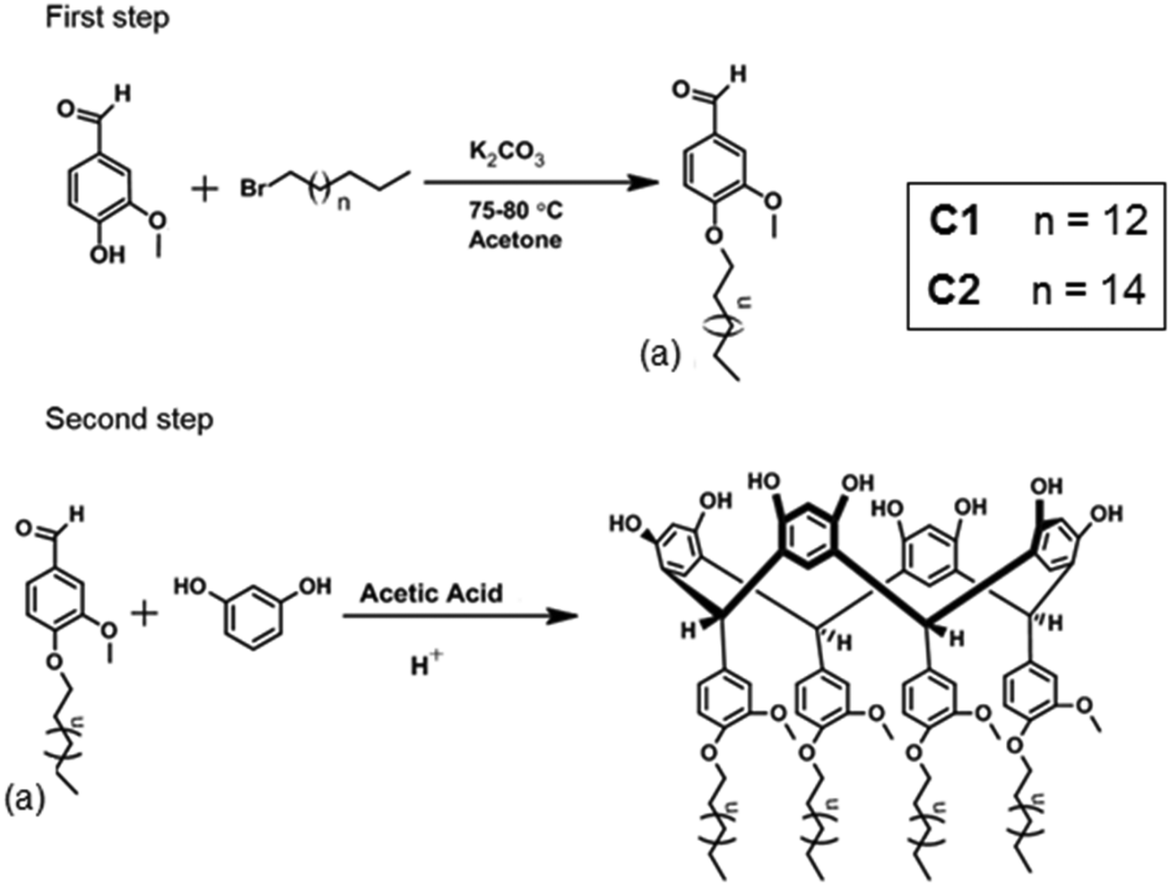

Scheme 1 Synthesis of a functionalized calix[4]resorcinarene macrocycle through a two-step reaction.

2.2. Absorption spectroscopy in THF and THF/H₂O mixtures and aggregation

The calix[4]resorcinarene macrocycle compound, C2, experiences some minor absorbance changes within 1–24 h after dissolution in THF or THF/H₂O mixtures, like the absorbances changes experienced by the macrocycle C1 in the same time period,³⁴ related to aggregation phenomena.^34,35 Consequently, all experiments described in this study were conducted only after the absorbance spectra of the solutions had become stable. To achieve this, C2 solutions were prepared and allowed to stabilize for 24 hours before experimentation.

The macrocycle C2, a calix[4]resorcinarene, exhibits a strong ultraviolet absorption peak when dissolved in THF at 285 nm, with a less pronounced shoulder at 291 nm. These observations were consistent across a concentration range of 1–5 × 10⁻⁵ M. At higher concentrations (above 10⁻⁴ M), a broad, weak absorption signal appeared between 330 and 600 nm (Fig. 1 and Fig. S5, ESI†). The overall absorption pattern of C2 closely resembles that of C1³⁴ and that of a related compound, resorcin[4]arene with R = CH₃–(CH₂)₁₄, with the same UV-vis spectrum.³⁶

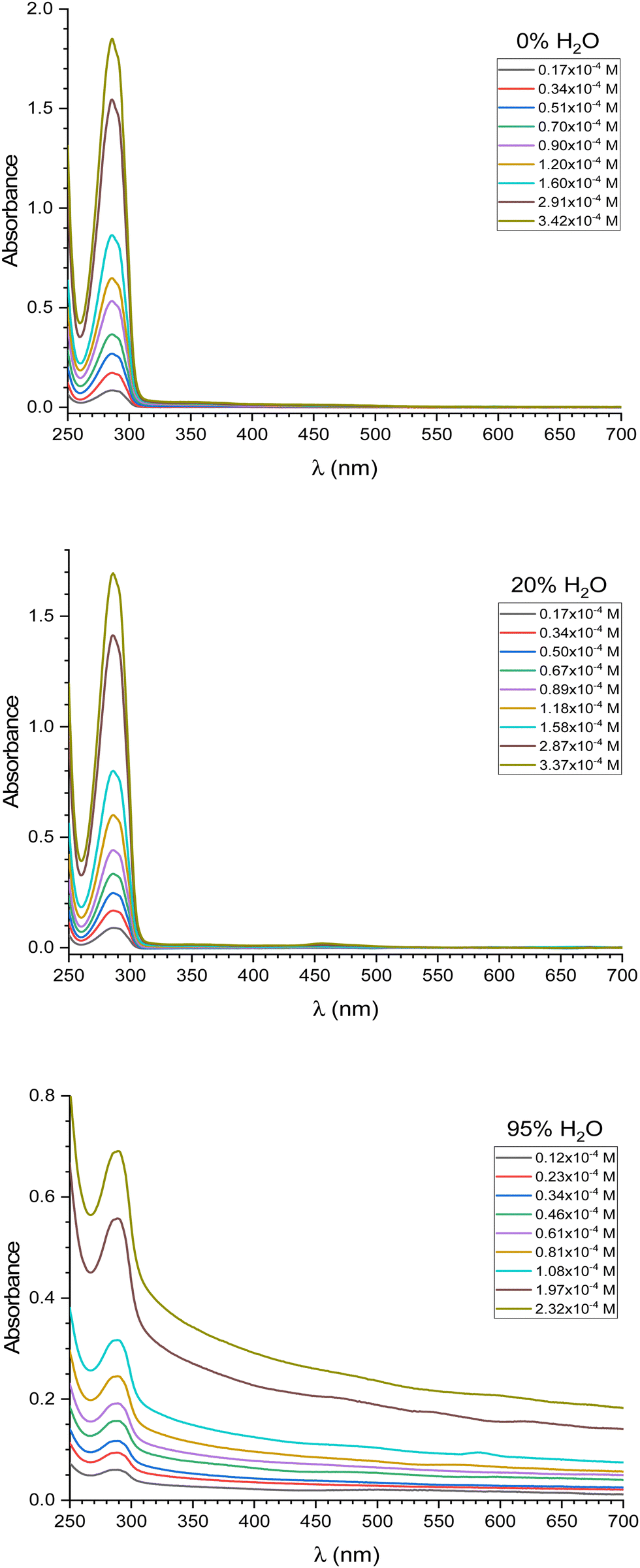Fig. 1 Absorption spectra of C2 at several concentrations in THF/H₂O mixtures.

Given their structure, resorcin[4]arenes like C1 or C2, lacking chromophoric groups, are expected to be colorless.^36,37 However, it was observed that increasing the concentration of these compounds above a certain point led to a weak absorption in the visible spectrum. This phenomenon, also seen in C1,³⁴ is attributed to molecular aggregation. To further investigate this, the absorption spectra of C2 were measured in THF solutions with varying water content. The spectra were recorded for solvent mixtures with H₂O proportions of 0, 20, 33, 47, 53, 60, 67, 75, 82, 88, and 95%. As the water content increased from 0 to 20%, a similar absorption tail in the visible region grew, comparable to the behavior of C1.³⁴ Additionally, increasing the concentration of C2 in either pure THF or THF with 20% water resulted in a stronger absorption at 355 nm. At water concentrations exceeding 33%, similar to observations with C1,³⁴ an increase in C2 concentration led to amplified absorbance between 400 and 700 nm, indicating enhanced aggregation. Comparative analysis of C1 and C2 absorption spectra under equivalent experimental conditions (concentrations and solvent mixtures, as depicted in Fig. 1 and Fig. S5, ESI†) revealed subtle disparities suggesting distinct aggregation behaviors. Consequently, we employed principal component analysis (PCA) to comprehensively examine the entire dataset of C1 and C2 absorption spectra. For the PCA, we incorporated additional data for C1 at 75%, 82%, and 88% water content, which were not included in our previous report.³⁴

2.3. Principal component analysis

The entire absorption matrix, denoted by A, encompassing a complete set of around 200 absorption spectra between 250 and 700 nm, was subjected to PCA using two different strategies. This matrix corresponds to the full range of experimental conditions, including solvent compositions varying from 0% to 95% water in THF, and analytical concentrations (C₀) ranging from 10 to 300 μM for compounds C1 and C2. The first PCA was performed on the original data, represented by the matrix A. The second PCA utilized the ratio matrix, A/C₀, effectively performing PCA on the apparent extinction coefficient matrix, E_app.

In matrix representation, the model with a given number of components can be expressed by the following equation: X = TP^T + E, where X represents the centered data matrix, T is the scores matrix, P^T is the transpose of the loadings matrix, and E is the error matrix. In the present work, we used two alternative definitions of X. If the original data is denoted by A, then X = A − Ā, where Ā is the mean absorption spectrum matrix. Similarly, if the original data represents apparent extinction coefficients and is denoted by E_app, then X = E_app− Ē_app, where Ē_app is the mean apparent extinction coefficient spectrum.

Within the PCA framework, the scores (T) and loadings (P) matrices form the crux of the analysis, capturing the most informative, structured variation within the data. These matrices can be likened to a compressed map, highlighting the key features and trends present in the original high-dimensional data space. The residual matrix (E) represents the unexplained variation, often referred to as noise, which cannot be effectively modeled by the chosen number of principal components. The core structure of the original data can be reconstructed by multiplying the scores and transposed loadings matrices (TP^T). Ideally, if the proper number of principal components is chosen, this reconstruction minimizes the residual matrix, leaving only a minimal amount of random error that is not amenable to meaningful interpretation within the context of the analysis.

Application of PCA revealed that most of the variabilities linked to either the A or E_app matrices could be adequately represented by keeping only two principal components. Regarding the A matrix, PC1 accounted for 85% of the variance, while PC2 captured the rest. Conversely, for the ratio matrix E_app, the distribution of explained variance shifted slightly, with PC1 explaining 82% and PC2 explaining 17% of the variance.

2.3.1. Decomposition of the A and E_app matrices into principal components. Fig. 2(a) and (b) depict the PC2 vs. PC1 scores plot for compounds C1 and C2, representing a compressed map of the data across all experimental conditions. ESI,† Fig. S6–S27 visualize the contributions to the core data structure reconstructed by each principal component (PCi). These figures present the spectral profiles obtained as (TP^T + Ā vs. λ) as a function of both analytical concentration (C₀) and solvent composition. While a direct physical interpretation of the principal components (PCs) can be challenging, PCA enables us to identify underlying patterns and trends. PC1 primarily accounts for the overall increase in spectral intensity with concentration, while PC2 mainly captures the changes in the spectral features induced by variations in environmental conditions. Positive PC2 scores correspond to a relative increase in the absorptive contribution, whereas negative scores indicate a greater dispersive contribution to the overall absorption spectrum.

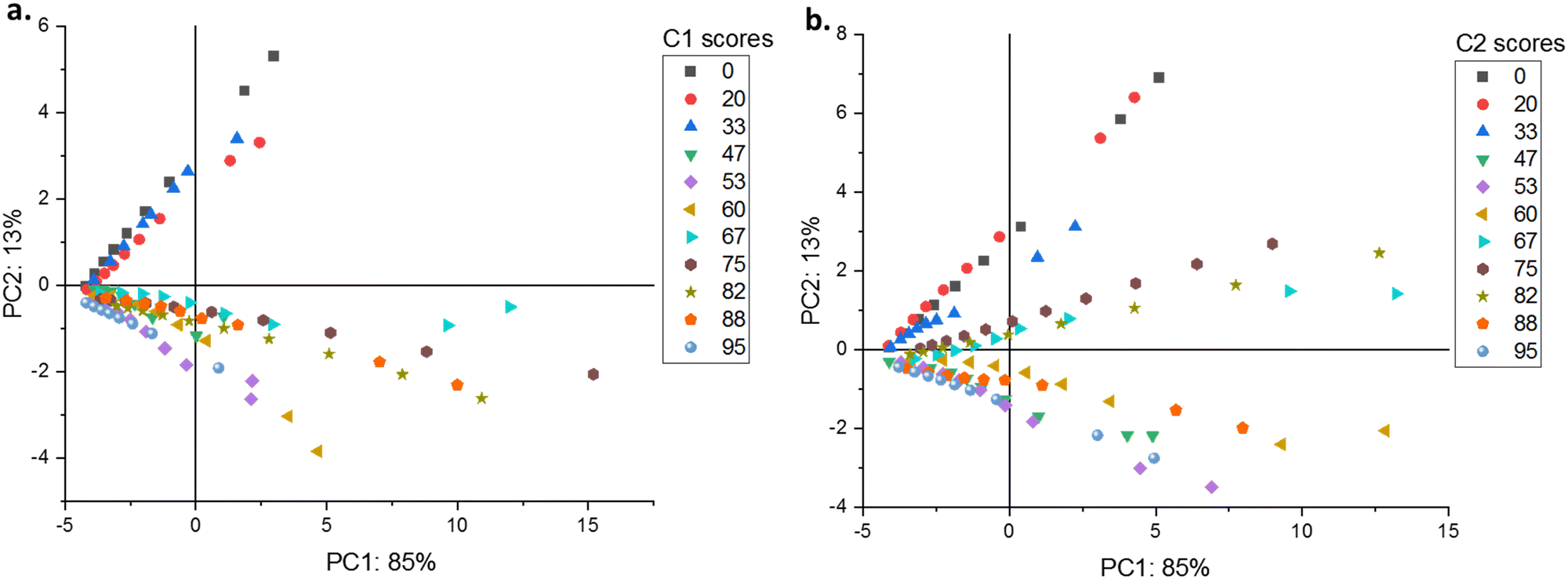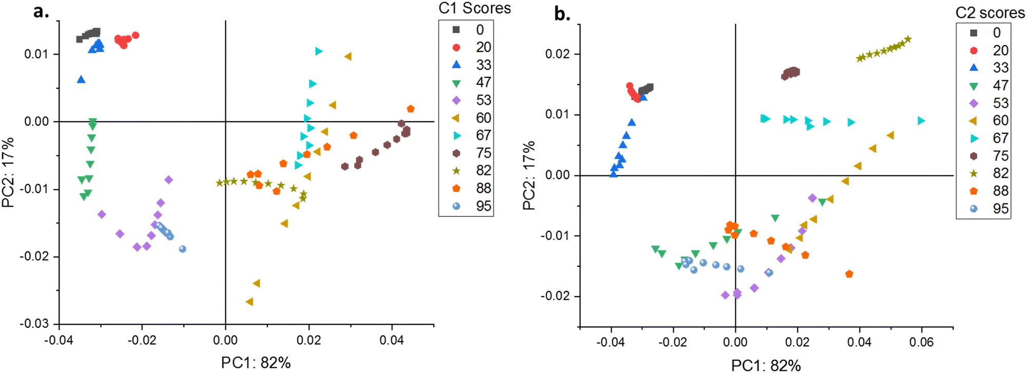
Fig. 2 (a) PC2 vs. PC1 scores for C1. (b) PC2 vs. PC1 scores for C2.

For compound C1, the PC2 vs. PC1 scores plots reveal distinct trends based on solvent water content. For water contents between 0% and 33%, the slopes are positive, with the steepest slope observed at 0% and the shallowest at 20%. Interestingly, the slopes become consistently negative for water contents exceeding 47%.

In contrast to compound C1, the PC2 vs. PC1 scores plots of compound C2 exhibit a distinct pattern. The slopes are positive and nearly identical at 0% and 20% water content. The slope becomes slightly less positive at 33% water content. Conversely, water contents of 47%, 60%, 88%, and 95% show negative slopes. However, while the initial slopes for C2 are positive for water contents ranging from 67% to 82%, they differ from the consistently negative slopes seen for C1.

A more detailed analysis of PC behavior is achieved by plotting each score (PCi) for a given solvent composition as a function of analytical concentration (C₀). Fig. 3(a)–(c) depict these plots for compound C1. In Fig. 3(a), PC1 and PC2 scores exhibit a linear increase with increasing C₀ for solvent compositions of 0% and 20% water. At 33% water content, the initially linear trend deviates downward, indicating a decrease in the slope and a downward curvature at higher concentrations exceeding 150 μM. Fig. 3(b) and (c) reveal distinct trends for higher solvent content (47–60% water in THF). While PC1 scores maintain a linear increase with C₀, PC2 scores exhibit a negative slope. Similarly, for solvent compositions between 67% and 95% water, PC1 scores continue their linear rise with C₀, whereas PC2 scores display a negative slope.

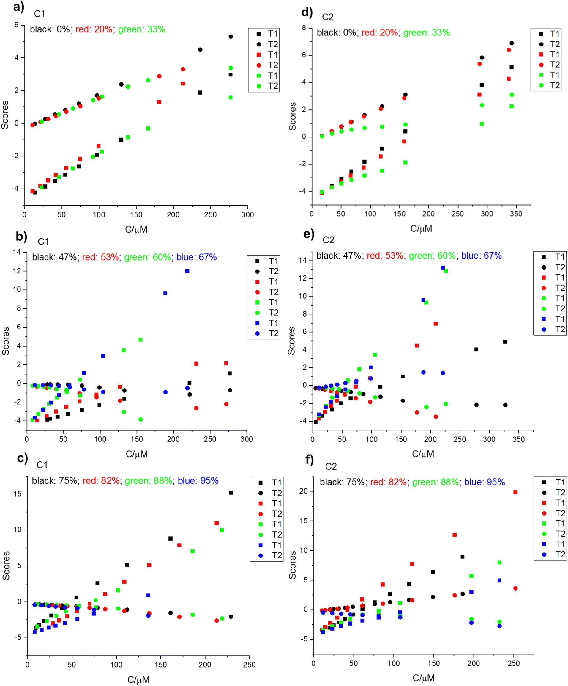Fig. 3 PCi vs. C₀ for different H₂O contents in THF; (a) and (d) for 0, 20, 33%; (b) and (e) for 47, 53, 60, 67%; (c) and (f) for 75%, 82%, 88%, 95%.

Compound C2 exhibits analogous behavior in its first principal component, as evidenced by the PC1 vs. C₀ plots across different water contents (Fig. 3(d)–(f)). In contrast to the C1 pattern, PC2 scores for C2 exhibit a more complex profile. The slopes fluctuate, transitioning from positive within the 0–30% water range to negative between 47% and 60% water. Subsequently, they become positive again from 67% to 82%, only to revert to negative between 88% and 95%. Table 1 summarizes the estimated initial slopes of the plots of PC1 and PC2 scores against the analytical concentrations of C1 and C2.

Table 1 Estimated^a initial slopes for PC1 and PC2 scores vs. C₀ plots. The initial slopes were calculated by linear regression analysis taking the appropriate number of points to preserve the linear trend (at least six points were included in this calculation)

% H2O	dT1/dC0, C1	dT2/dC0, C1	dT1/dC0, C2	dT2/dC0, C2
a Relative errors where, in all cases, lower than 6.5%.
0	0.0275	0.0202	0.0316	0.0211
20	0.0324	0.0170	0.0265	0.0196
33	0.0254	0.0178	0.0177	0.0097
47	0.0198	−0.0059	0.0392	−0.0081
53	0.0321	−0.0139	0.0502	−0.0162
60	0.0658	−0.0168	0.0682	−0.0125
67	0.0751	−0.0084	0.0581	0.0119
75	0.0840	−0.0081	0.0725	0.0162
82	0.0770	−0.0116	0.0958	0.0155
88	0.0622	−0.0071	0.0483	−0.0053
95	0.0394	−0.0117	0.0356	−0.0091

---

The core data structures reconstructed by principal component PCi for C1 and C2 (Fig. S6–S27, ESI†) exhibit shared spectral characteristics and are thus discussed collectively. Across all solvent mixtures (0–95% water in THF), the TP^T + Ā spectral contributions associated with PC1 comprise an absorption band centered at ∼286 nm, superimposed on a scattering continuum extending across the entire wavelength range. This scattering component's wavelength dependence aligns with Mie scattering theory.³⁸

I = Cλ^−k (1)

where intensity is inversely proportional to wavelength raised to the power k. The constant C in eqn (1) is valid under conditions of uniform particle and medium dispersion. While Rayleigh scattering (k = 4) applies to smaller particles, Mie scattering (k < 4) is relevant for larger ones. However, in media containing a distribution of particle sizes and irregular shapes, both C and k become size-dependent, complicating scattering models. For PC1, both the 286 nm absorption intensity and scattering contribution increase monotonically with C₀. The contribution associated with PC1 consistently increases more than that of PC2 with increasing analytical concentration, primarily because PC1 accounts for most spectral alterations induced by concentration changes.

Inspection of Fig. S6–S27 (ESI†) reveals that the scattering continuum associated with PC2 is flatter than that of PC1, indicating a lower k value for PC2 within the solvent composition range analyzed. Comparison of PC1 and PC2 spectral trends suggests that the underlying data structures of C1 and C2 can be categorized into four solvent ranges: (a) 0–33%, (b) 47–60%, (c) 67–82%, and (d) 88–95%. Noteworthy, this behavior is in line with the results shown in Fig. 3 and the data presented in Table 1.

2.3.2. Decomposition of the E_app matrix into principal components. Fig. 4 depicts the PC2 vs. PC1 scores plot for compound C1 and C2, representing a compressed map of the data across all experimental conditions. ESI,† Fig. S28–S49 visualize the core data structure reconstructed by each principal component (PCi). These figures present the spectral form (TP^T + Ē_appvs. λ) as a function of both analytical concentration (C₀) and solvent composition.

Fig. 4 (a) PC2 vs. PC1 scores for C1. (b) PC2 vs. PC1 scores for C2.

Fig. 4 differs fundamentally from Fig. 2 due to the transformation of the A matrix into E_app, which eliminates PC variance arising from the overall increase of spectral signals associated with higher analytical concentrations.

For compound C1, the PC2 vs. PC1 scores plot (Fig. 4(a)) is divided into four quadrants. The upper left quadrant contains data points representing the 0–33% water in THF range (negative PC1, positive PC2). The lower left quadrant includes data for 47%, 53%, and 95% water in THF (negative PC1 and PC2). The upper right quadrant, sparsely populated, contains a small subset of data with positive PC1 and PC2 scores. The lower right quadrant encompasses data for 60%, 67%, 75%, 82%, and 88% water in THF (positive PC1, negative PC2). For compound C2, the PC2 vs. PC1 scores plot (Fig. 4(b)) shows a different distribution. The upper left quadrant contains data points representing the 0–33% water in THF range. The upper right quadrant includes data for 67%, 75%, 82%, and a portion of the 60% water in THF data. The remaining solvent data are distributed across the lower left and right quadrants.

To provide a more detailed examination of PC behavior, the PC2 vs. PC1 scores plots (previously shown collectively in Fig. 4) are presented individually for each solvent composition as a function of analytical concentration (C₀) in Fig. S50–S71 (ESI†). In each of these figures, the analytical concentration is labeled directly above the corresponding data point on the PC2 vs. PC1 scores plot.

For C1 and C2, Fig. S50–S71 (ESI†) reveal complex patterns in the relationship between PC1 and PC2 scores as C₀ steadily increases. While some plots show initial steady increases (e.g., Fig. S50, ESI†) or decreases (e.g., Fig. S62, ESI†) in PC2 scores with rising PC1 values, all eventually exhibit more intricate behaviors within specific C₀ ranges. These include abrupt drops, loop-like structures, and even instances of double reversals where the trajectory reverses direction twice. Table 2 provides estimated concentration ranges for these potential turning points.

Table 2 Estimated concentration ranges for potential turning points

% H2O (v/v)	C1	C2
	C 0/μM	C 0/μM
0	130–236	160–291
20	99.6–181	118–158
33	65–92	160–291
47	133–222	153–278
53	95–127	97.5–177
60	—	106–193
67	104–189	74–98.6
75	18.9–27; 161–229	31.2–39.1
82	55.9; 171–213	—
88	102–186	108–197
95	56.1–74.8	81.2–108

---

The core data structures reconstructed by principal component PCi for C1 and C2 (Fig. S28–S49, ESI†) exhibit shared spectral characteristics and are thus discussed collectively. Comparison of the spectral contributions associated with PC1 and PC2 reveals that both exhibit absorption bands centered around 287 nm, overlaid by broad scattering continuums. However, the portion of the signals accounted for PC1 exhibits a less absorptive contribution than that of PC2. In addition, a detailed inspection of the spectral region dominated by scattering effects also shows that the changes in PC1 scores account for those signals associated with higher k values of eqn (1), whereas the changes in PC2 scores mainly describe scattering signals that correspond to lower values of the exponent.

The PCA analyses of matrices A and E_app provide complementary insights. While the PCA of matrix A emphasized the differences between C1 and C2 at low analyte concentrations, the PCA of E_app matrices enabled a comprehensive analysis across all solvent concentrations and revealed the occurrence of turning points. This indicates that phase transitions occur even in pure THF, where scattering is observed at concentrations as low as 70 mM. Although our PCA analysis cannot provide precise CMC values, it suggests multiple phase transitions leading to the final micellar structures (see DLS results below).

2.4. Dynamic light scattering

Dynamic light scattering (DLS) confirmed the presence of C2 aggregates, like previous observations for C1,³⁴ with substantial size variability and large particles detected in pure THF. However, as with C1, data quality precluded reporting precise hydrodynamic diameter (d_h) values. Detailed data are presented in Fig. S72–S81 and Tables S1–S10 (ESI†). Table 3 summarizes DLS data for C1 and C2 at 33, 53, 67, 82, 88, and 95% water in THF.

Table 3 Hydrodynamic radii (DLS) from solutions of C1 and C2 prepared from THF or THF/H₂O mixtures

Water (%)	C1 DLS dh	C2 DLS dh
0	—	—
33	Trimodal distribution	Trimodal distribution
	3.51 ± 0.09 nm (84.1%)	3.42 ± 0.07 nm (78.4%)
	536 ± 79 nm (11.9%)	348 ± 39 nm (18.7%)
	5204 ± 203 nm (3.9%)	5448 ± 81 nm (2.9%)
	P.I. = n.d.	P.I. = n.d.
53	Bimodal distribution	Bimodal distribution
	1001 ± 145 nm (94.4%)	944 ± 43 nm (99%)
	2.88 ± 0.04 nm (5.3%)	5514 ± 66 nm (1%)
	P.I. = n.d.	P.I. = 0.32 ± 0.03
67	Unimodal distribution	Trimodal distribution
	152 ± 2 nm (100%)	110 ± 10 nm (16.6%)
	P.I. = 0.06 ± 0.02	470 ± 26 nm (82.6%)
		5547 ± 20 nm (0.8%)
		P.I. = 0.53 ± 0.05
82	Bimodal distribution	Unimodal distribution
	165 ± 6 nm (96.9%)	143 ± 3 nm (100%)
	4687 ± 296 nm (3.1%)	P.I. = 0.14 ± 0.01
	P.I. = 0.23 ± 0.01
95	Unimodal distribution	Unimodal distribution
	166 ± 2 nm	140 ± 1 nm (100%)
	P.I. = 0.1 ± 0.1	P.I. = 0.113 ± 0.007

---

DLS results for C2 revealed a trimodal size distribution at 33% water, with d_h values of 3.42 ± 0.07 nm (78.4%), 348 ± 39 nm (18.7%), and 5448 ± 81 nm (2.9%). Like C1, the largest aggregates were of minor importance. However, the relative abundance of the major component (3.42 nm) was lower for C2 compared to C1 (3.51 nm, 84%), while the middle size component of C2 (348 nm) was more prominent than that of C1 (536 nm). Notably, aggregate sizes for C1 and C2 were comparable at this water content. At 53% water, C2 exhibited a nearly unimodal distribution with d_h of 944 ± 43 nm (99%) and a minor population at 5514 ± 66 nm (1%), accompanied by a high P.I. of 0.32 ± 0.03. Regarding overall size, unlike C1, C2 lacked the small aggregates present in C1 but retained a small population of very large aggregates. A virtually bimodal distribution emerged at 67% water for C2, with d_h values of 110 ± 10 nm (16.6%) and 470 ± 26 nm (82.6%), and a minor population at 5547 ± 20 nm (0.8%). The high P.I. of 0.53 ± 0.05 indicated significant polydispersity. Smaller micellar aggregates (∼110 nm), most likely precursors to the dominant species at higher water content, coexisted with larger, dominant aggregates (∼470 nm). Negligible amounts of very large aggregates persisted. This behavior contrasts with the unimodal size distribution of C1 at 67%. It is worth noting that, although DLS and UV-vis results cannot be straightforwardly correlated, the latter contrast is also observed in Fig. 4, where C1 and C2 exhibit a much distinct pattern at 67% water. Unimodal distributions were observed at 82% and 95% water for C2, with d_h values of 143 ± 3 nm (P.I. = 0.14 ± 0.01) and 140 ± 1 nm (P.I. = 0.113 ± 0.007), respectively. While both C1 and C2 showed unimodal distributions at these water contents, C1 exhibited larger micellar sizes.

The polydispersity index (P.I.) is a measure of the distribution of particle sizes in a sample. A P.I. above 0.5 indicates a broad range of particle sizes.³⁹ The DLS results show that C2 in general has a higher P.I. than C1, suggesting a broader range of particle sizes in C2. In addition, the highest P.I. values are achieved at lower water contents for C2 (53–67%) compared to C1 (82%).

When the DLS sizes of the more important contribution to the scattering (i.e. that contributing above 80% to the total scattering) are represented vs. % of water content, a plot like that of Fig. 5 is obtained. This figure shows the difference between C1 and C2 behaviors of DLS sizes versus water content. In line with the results from the PCA of UV-vis data presented in Fig. 4, the major differences between the behavior of C1 and C2 were observed at 67% water content.

Fig. 5 Behavior of major DLS sizes vs. % H₂O for C1 and C2.

2.5. Fluorescence

Upon excitation at its high-energy absorption maximum (λ_ex = 285 nm), C2 in pure THF exhibited fluorescence emission centered at approximately 315 nm (Fig. 6(a)), with similar spectral characteristics to the fluorescence of C1.³⁴ The quenching of the fluorescence of C1 and C2 was studied either by measuring the fluorescence quantum yields by the integrating sphere method and/or by measuring the emission spectra at different water content in THF (for the complete absorption and emission spectra recorded, please refer to Fig. S82–S85, ESI†).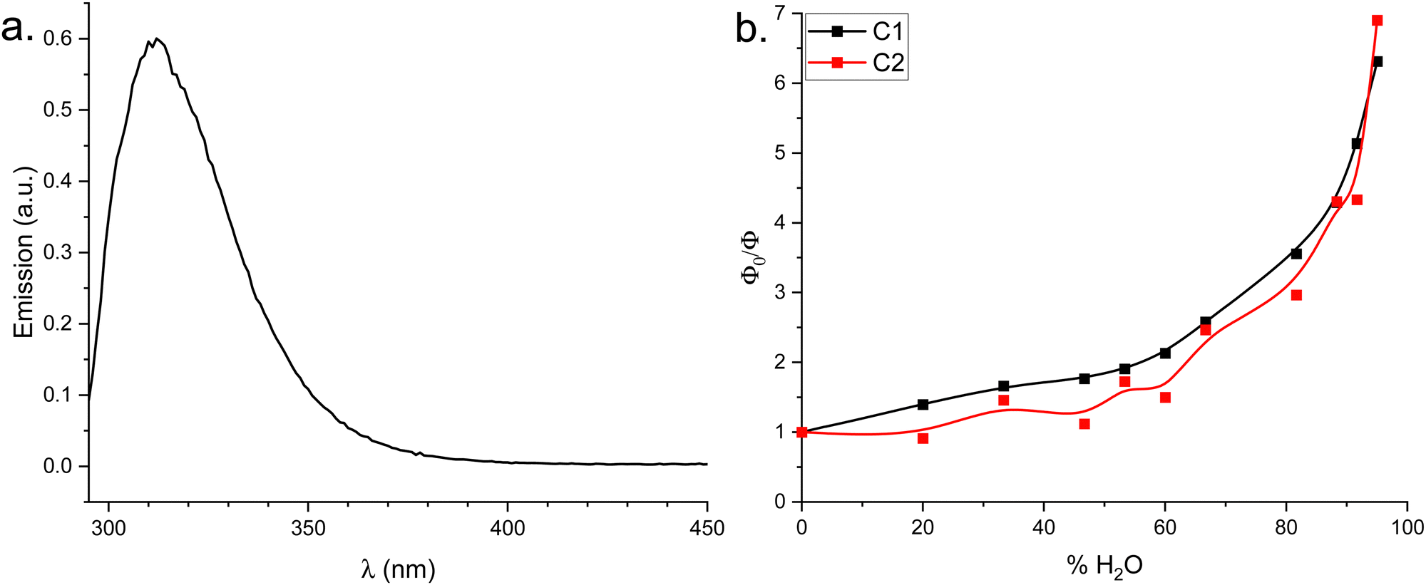

Fig. 6 (a) Luminescence spectra of C2 in pure THF; (b) Φ₀/Φ values as a function of % H₂O for C1 and C2.

Progressive water addition induced fluorescence quenching, resulting in a tenfold intensity reduction at 95% water content compared to the anhydrous solution. Luminescence quantum yields, determined via the integrating sphere method, are presented in Table 4 as a function of water percentage. Plots of Φ₀/Φ versus water content for C1 and C2 (Fig. 6(b)) deviated upward from linearity even at low water percentages. This observation in addition to the luminescence lifetimes behavior (see below) suggest the contribution of both dynamic and static quenching phenomena. Two key observations emerged from these plots: (i) an initially steeper slope for C1 compared to C2, (ii) two distinct increases in slope, occurring around 60% and above 80% water content, and (iii) a steeper slope for C2 than C1 at high water content (i.e., above 80%).

Table 4 Fluorescence quantum yields (Φ), luminescence lifetimes (τ_short and τ_long), amplitude average lifetimes (τ_ave-amp), radiative (k_r), and radiationless (k_nr) deactivation rate constants of C2 in THF at different % H₂O

% H2O	Φ	τ short/ns	τ long/ns	τ ave-amp/ns	k r/10^8 s^−1	k nr/10^9 s^−1
0	0.15 ± 0.02	0.54 ± 0.02	1.46 ± 0.04	0.75 ± 0.03	1.98 ± 0.09	1.13 ± 0.05
20	0.16 ± 0.02	0.54 ± 0.02	1.50 ± 0.04	0.75 ± 0.01	2.06 ± 0.05	1.13 ± 0.02
33	0.096 ± 0.009	0.50 ± 0.02	1.48 ± 0.04	0.73 ± 0.03	1.32 ± 0.06	1.24 ± 0.06
47	0.13 ± 0.01	0.35 ± 0.07	1.43 ± 0.09	0.7 ± 0.1	1.8 ± 0.3	1.2 ± 0.2
53	0.082 ± 0.008	0.28 ± 0.04	1.34 ± 0.09	0.55 ± 0.07	1.5 ± 0.2	1.7 ± 0.2
60	0.094 ± 0.009	0.29 ± 0.08	1.2 ± 0.1	0.5 ± 0.1	2.1 ± 0.5	2.0 ± 0.5
67	0.057 ± 0.006	0.28 ± 0.02	1.18 ± 0.04	0.44 ± 0.04	1.3 ± 0.1	2.1 ± 0.2
82	0.048 ± 0.004	0.26 ± 0.06	1.0 ± 0.1	0.37 ± 0.07	1.3 ± 0.3	2.6 ± 0.5
88	0.033 ± 0.003	0.22 ± 0.02	1.05 ± 0.06	0.28 ± 0.03	1.2 ± 0.1	4.5 ± 0.4
92	0.033 ± 0.003	0.19 ± 0.02	1.1 ± 0.1	0.23 ± 0.02	1.4 ± 0.3	4.1 ± 0.4
95	0.020 ± 0.002	0.15 ± 0.01	0.96 ± 0.08	0.19 ± 0.02	1.1 ± 0.2	5.2 ± 0.7

---

Fluorescence decay of C2 was best described by a biexponential function. The longer lifetime (τ_long) decreased from 1.5 to 1.0 nanoseconds across the 0–95% water content range, while the shorter lifetime (τ_short) also decreased, varying between 0.5 and 0.2 nanoseconds (Table 4). At 0% water, τ_long contributed 44% to the total relative amplitude, with τ_short contributing 56%. These relative amplitudes remained relatively constant up to 67–75% water, but thereafter, the contribution of τ_long decreased to 23% at 95% water, accompanied by a corresponding increase in the contribution of τ_short to 77%.

Amplitude-averaged lifetimes (τ_ave-amp), calculated from τ_long and τ_short, decreased from 0.75 ns (0–47% water) to 0.2 ns at 95% water. Using τ_ave-amp, average radiative (k_r) and non-radiative (k_nr) deactivation rate constants were determined according to the following equations:

k_r = ϕ_f/τ_ave-amp

k_nr = (1 − ϕ_f)/τ_ave-amp

In anhydrous THF, k_r and k_nr values for C2 were determined to be 1.98 × 10⁸ and 1.13 × 10⁹ s⁻¹, respectively. Upon water addition, k_r decreased to 1.1 × 10⁸ s⁻¹, while k_nr increased to a range of 1.13 to 5.2 × 10⁹ s⁻¹ (Table 4). The luminescence decay behavior of C2 resembled that of C1³⁴ although a more pronounced decrease in lifetimes was observed during quenching, indicating a more significant contribution of the dynamic quenching component to the overall quenching process in C2 compared to C1.

A joint multivariate curve resolution (MCR) analysis of the full absorbance and fluorescence matrices (Fig. S82–S85, ESI†) revealed three primary spectral contributions, hereafter labeled as Sp1, Sp2, and Sp3 (Fig. 7). The first exhibited a relatively pure absorption spectrum and a high quantum yield, while the second showed an almost pure absorption spectrum but a significantly lower quantum yield (approximately 15 times less). The third contribution displayed a predominantly dispersive spectrum with some absorption and a quantum yield somewhat higher than the second. The total fluorescence demonstrated a steep decline between 47% and 60% water content, primarily due to the decrease of the first contribution. The scattering signal peaked at 60% water, but this did not correspond to a fluorescence maximum, suggesting a complex interplay between absorption, emission, and scattering processes. The bottom-center graph suggested a correlation between the high absorptive/low emissive contribution and the state of aggregation as the water percentage increased.

Fig. 7 MCR analysis of the absorbance and fluorescence: (a) absorption spectra of contributions Sp1, Sp2 and Sp3; (b) emission spectra of contributions Sp1, Sp2 and Sp3; (c) Sp1 relative contribution vs. % H₂O; (d) Sp2 relative contribution vs. % H₂O; (e) Sp3 relative contribution vs. % H₂O.

2.6. AFM analysis of aggregates

Previously reported AFM analysis of an amphiphilic calixarene revealed two distinct particle populations. Surprisingly, the first consisted of roughly 200 nm diameter spherical objects. More unexpectedly, a second type of structure was observed: a layered system with a thickness of 1.5–2 nm, resembling a supported lipid bilayer.⁴⁰ The morphology of C1 and C2 aggregates was investigated using AFM. Samples were prepared by depositing solutions onto mica substrates and drying them under vacuum. In pure tetrahydrofuran (THF), AFM imaging of C1 showed flattened, round bilayer sheets with a trimodal size distribution with diameters varying from 300–600 nm and heights varying from 8–47 nm.³⁴ Notably, all clusters displayed significant flattening, reminiscent of supported lipid bilayers as described by Shahgaldian et al.⁴⁰ AFM imaging revealed that C2 formed a continuous layer on the mica surface, punctuated by depressions resembling a cluster of interconnected doughnuts (Fig. 8(a)).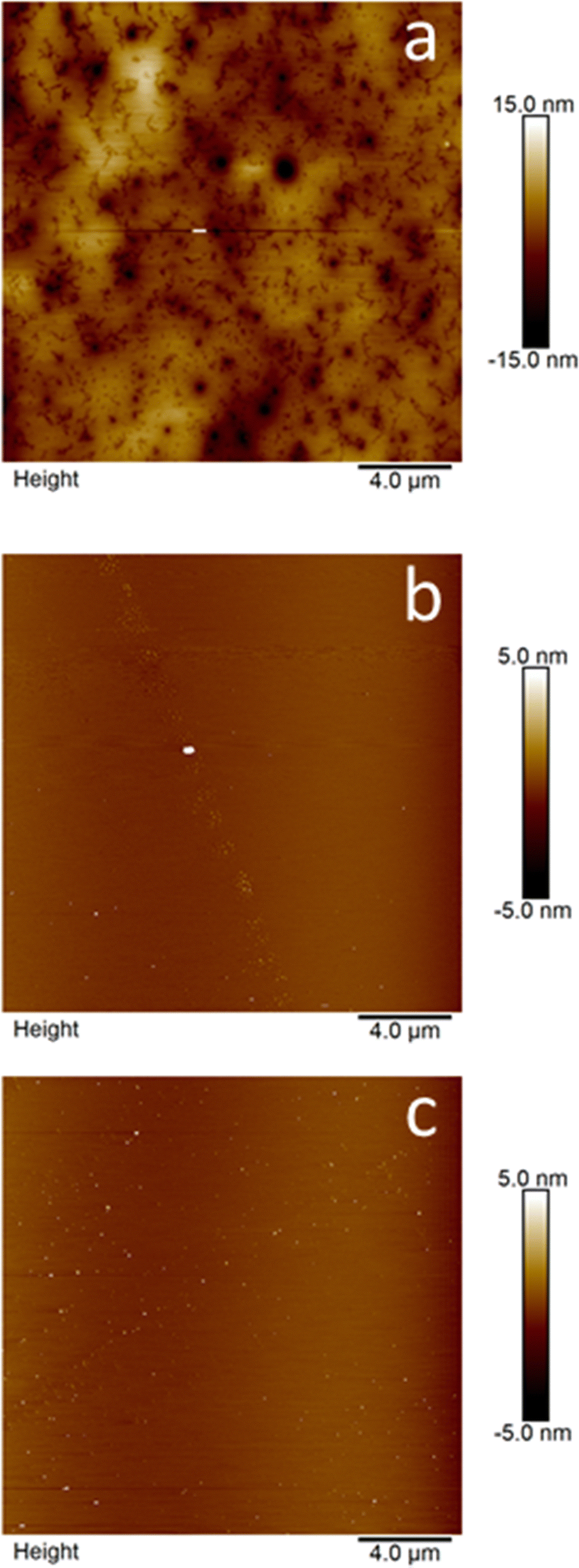

Fig. 8 AFM images of C2 in: (a) pure THF, (b) THF (47%)/H₂O (53%) and (c) THF (5%)/H₂O (95%).

At 53% water content (Fig. 8(b) and Fig. S86, ESI†), a marked decrease in both the number and size of larger clusters was observed. The distribution became predominantly unimodal with average dimensions of d = 150 ± 42 nm and h = 1.3 ± 0.7 nm, suggesting that water addition flattened and reduced the size of these clusters. Increasing the water content to 95% resulted in the near-complete elimination of large clusters (Fig. 8(c) and Fig. S87, ESI†). Instead, a pronounced unimodal distribution with significantly smaller dimensions emerged (d = 73 ± 18 nm, h = 3.7 ± 2.1 nm). Notably, the morphological characteristics of C2 observed in Fig. 8 and Fig. S86, S87 (ESI†) exhibit similarities to the self-assembly behavior of para-carboxy modified amphiphilic calixarene in water.⁴⁰

Table 5 summarizes the sizes of C2 aggregates measured by AFM, compared to those of C1. The trimodal distribution of flattened round bilayer sheets observed in C1 is not apparent in C2, which forms a continuous layer on the mica surface. This suggests increased aggregation in C2 owing to the longer carbon chains. Additionally, at 53% water content, the bilayer sheets in C2 are significantly smaller than those in C1, indicating a more pronounced aggregation towards micellar-like structures in C2. This finding is consistent with the larger values of the hydrodynamic diameter (d_h) for the major component of the scattering in DLS experiments for C2.

Table 5 Diameters and heights of the flattened round layer sheets (AFM) from solutions of C1 and C2 prepared from THF or THF/H₂O mixtures

Water (%)	C1 AFM diameter (nm)	C1 AFM height (nm)	C2 AFM diameter (nm)	C2 AFM height (nm)
0	605 ± 317	47 ± 34	—	—
	399 ± 99	15 ± 9
	336 ± 107	8 ± 5
53	302 ± 89	9 ± 5	151 ± 42	1.3 ± 0.7
95	72 ± 19	2.8 ± 0.5	73 ± 17	3.7 ± 2.1

---

2.7. Analysis of solvent-dependent aggregation

PCA analysis of absorption spectra, combined with DLS and AFM experiments, reveals the following insights into the aggregation behavior of C1 and C2 molecules in THF/H₂O mixtures:

1. Even in pure THF, resorcinarene molecules exhibit aggregation. This is evident from scattered light at low concentrations (70 μM) as observed by absorption spectroscopy and from the turning points in the PCA analysis at concentrations above 130 μM, indicating phase transitions.

2. In THF/H₂O mixtures with 33% water content, DLS experiments suggest the presence of small micelles (d_h 3.4–3.5 nm) as the dominant component (>80%). Additionally, large unilamellar vesicles (LUV) or giant unilamellar vesicles (GUV) with diameters of 536 nm for C1 and 348 nm for C2 are observed, along with minor components (3–4%) of very large GUV (5204 nm for C1 and 5448 nm for C2). Based on previous calculations³⁴ the small micelles likely contain 8–10 molecules. These giant structures are collectively named GV, but the experimental techniques employed do not distinguish between GUV, multilamellar vesicle (MLV), or multivesicular vesicle (MVV) (see Scheme 2 for a schematic representation of micelles, bilayers, and different types of vesicles and their size dimensions).

Scheme 2 Micelles, bilayers, vesicles and their characteristic dimensions.

3. At 53% water content, giant micelles (GM) become the dominant species in the size distribution, with diameters of 1001 and 944 nm for C1 and C2, respectively.

4. AFM images indicates that solvent evaporation induces the coalescence and flattening of solution aggregates. This is evident from the observed flattened structures with diameters significantly larger than their heights.

5. For C1, a unimodal distribution of sizes is observed from DLS experiments, varying from 152 nm at 67% water to 165–166 nm at 82–95% water. C2 shows a slightly different behavior, with a more gradual decrease in size from GUV to micelles as water content increases. At 67% water, the dominant aggregates for C2 are 470 nm, with smaller aggregates of 110 nm and a minor component of very large structures (5547 nm). This differential behavior of C1 and C2 upon water content is also evident in Fig. 5.

2.8. Aggregation caused quenching in THF/H₂O mixtures

Experiments employing absorption spectroscopy, dynamic light scattering, atomic force microscopy, and both steady-state and time-resolved fluorescence revealed the phenomenon of aggregation caused by quenching (ACQ) in C1 and C2 molecules due to increasing water content in THF/H₂O mixtures.

Φ ₀/Φ versus water content for C1 and C2 revealed subtle differences, which may be attributed to the effect of the chain length on the differential aggregation behavior observed by DLS, AFM, and PCA analysis of absorption spectra.

For instance, Fig. 5 shows that DLS sizes corresponding to the shorter-chain macrocycle (C1) drop more abruptly after water percent increases above 60% than the DLS of C2 (the macrocycle with the longer hydrocarbon chain). The distinct behavior is also revealed in the MCR analysis of the Sp3 component (the purely dispersive component) in Fig. 7, which shows a broader shape of Sp3 for C2 than for C1.

The analysis of fluorescence quenching as well as MCR results shows that:

1. The quenching of the fluorescence, evidenced either by the Φ₀/Φ plots (integrating sphere method, Fig. 6(b)) or the I₀/I or the A₀/A (intensities at the wavelength maximum or relative areas, Fig. S88 and S89, ESI†) has a relatively small slope which abruptly increases at water concentrations higher than 60% and with a steeper behavior for C2 than for C1.

2. Of the three contributions retrieved by MCR, the decline of Sp1 as water% increases accounts for the recorded fluorescence quenching.

3. The poorly emissive contribution Sp2, which has a small scattering component relative to the spectral component, increases abruptly at water concentrations above 53% for C2 and above 60% for C1, indicating differential micelle formation.

4. The Sp3 contribution, with spectral characteristics of a purely dispersive component, shows a water content percentage dependence more abrupt in C1 than in C2.

To a certain extent, although AFM and DLS sizes cannot be directly compared due to the flattening process in AFM due to solvent evaporation, this differential aggregation pattern shown by C1 and C2 was also observed by AFM, notably showing a trimodal distribution of flattened round bilayer sheets observed in C1 that is not apparent in C2, which forms a continuous layer on the mica surface. This suggests increased aggregation in C2 owing to the longer carbon chains. Additionally, at 53% water content, the bilayer sheets in C2 are significantly smaller than those in C1, indicating a more pronounced aggregation towards micellar-like structures in C2.

Furthermore, PCA shows a differential behavior of PC1 and PC2 versus C₀ in C1 and C2, especially in the different turning points concentration ranges. The deviation from a linear Stern–Volmer plot, even at low percentages of water, indicates the contribution of both static and dynamic quenching. The static quenching observed in the fluorescence of C1/C2 upon the addition of water is likely associated with an enhancement of nonradiative deactivation due to π–π stacking of neighboring resorcinol molecules. This stacking is exacerbated by H-bond formation and chromophore crowding as the water content is increased. Within the resorcinarene macrocycle clusters, there may be room for a specific number of chromophores whose fluorescence cannot be quenched by further addition of water, leaving some residual fluorescence at high water (95% or higher) contents.

Scheme 3 summarizes the experimental findings.

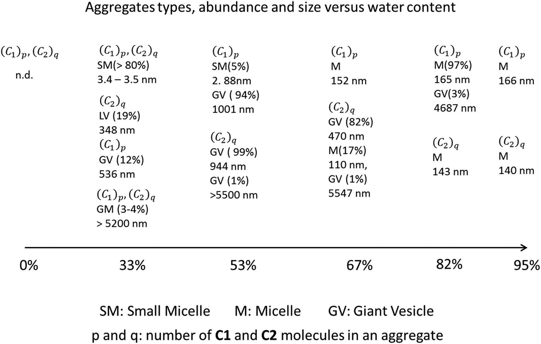Scheme 3 Influence of water content on aggregates types, abundance and sizes.

3. Conclusions

This investigation reveals a significant influence of water content on the self-assembly behavior of two resorcinarenes, C1 and C2. We demonstrate a water-mediated transformation, where resorcinarenes transition from forming large aggregates in THF/H₂O mixtures with water content below 60% to well-defined, smaller clusters as water concentration reaches 80–95%. Based on the experimental data, the addition of water to THF/H₂O mixtures leads to the aggregation of C1 and C2 molecules, with the chain length influencing the aggregation behavior. MCR analysis reveals distinct species contributing to fluorescence quenching and aggregation. The static quenching contribution observed is probably due to p–p stacking. C1 and C2 exhibit different aggregation patterns, with C2 showing a more pronounced tendency towards micellar-like structures at higher water concentrations.

This precise control over C1 or C2 self-assembly is accompanied by a phenomenon known as aggregation-induced quenching (ACQ), which effectively modulates the fluorescence intensity. While ACQ may initially appear to be a limitation, it presents a unique opportunity for sensor design. Prior research has established the utility of ACQ in calixarenes and resorcinarenes for selective detection of specific targets, including Cu(II) and Co(II) ions and organic pollutants like 4-nitrotoluene. Our findings suggest that these resorcinarenes, with their water-tunable ACQ, possess significant potential as a platform for the development of next-generation sensors with precise fluorescence control.

Data availability

The data supporting this article have been included as part of the ESI.†

Conflicts of interest

There are no conflicts to declare.

Acknowledgements

This work was supported in part by CONICET (PIP 112-2013-01-00236CO), ANPCyT (PICT 2018-03341) and UNLP (11/X779 and 11/X679) Argentina. E. W. is a Research Member of CONICET (Argentina). M. V. S. thanks ANPCyT and CONICET for a research scholarship. EC is acknowledged for the INFUSION project grant N. 734834 under H2020-MSCA-RISE-2016. We thank Dr Iván Maisuls from University of Münster, WWU Institute of Inorganic and Analytical Chemistry for performing ESI-HR-MS and EA analyses.

References

1. E. Weiand, F. Rodriguez-Ropero, Y. Roiter, P. H. Koenig, S. Angioletti-Uberti, D. Dini and J. P. Ewen, Effects of surfactant adsorption on the wettability and friction of biomimetic surfaces, Phys. Chem. Chem. Phys., 2023, 25, 21916–21934.
2. Z. Sumer and A. Striolo, Manipulating molecular order in nematic liquid crystal capillary bridges: Via surfactant adsorption: Guiding principles from dissipative particle dynamics simulations, Phys. Chem. Chem. Phys., 2018, 20, 30514–30524.
3. H. Lee and T. J. Jeonb, The binding and insertion of imidazolium-based ionic surfactants into lipid bilayers: The effects of the surfactant size and salt concentration, Phys. Chem. Chem. Phys., 2015, 17, 5725–5733.
4. A. M. S. Jorge, G. M. C. Silva, J. A. P. Coutinho and J. F. B. Pereira, Unravelling the molecular interactions behind the formation of PEG/PPG aqueous two-phase systems, Phys. Chem. Chem. Phys., 2024, 26, 7308–7317.
5. Y. Han and Y. Wang, Aggregation behavior of gemini surfactants and their interaction with macromolecules in aqueous solution, Phys. Chem. Chem. Phys., 2011, 13, 1939–1956.
6. A. Bhadani, M. Tani, T. Endo, K. Sakai, M. Abe and H. Sakai, New ester based gemini surfactants: the effect of different cationic headgroups on micellization properties and viscosity of aqueous micellar solution, Phys. Chem. Chem. Phys., 2015, 17, 19474–19483.
7. J. Penfold and R. K. Thomas, Phys. Chem. Chem. Phys., 2022, 24, 8553–8577.
8. M. Dasgupta and N. Kishore, Establishing Structure Property Relationship in Drug Partitioning into and Release from Niosomes: Physical Chemistry Insights with Anti-Inflammatory Drugs, J. Phys. Chem. B, 2017, 121, 8902–8918.
9. D. J. Speer, M. Salvador-Castell, Y. Huang, G. Y. Liu, S. K. Sinha and A. N. Parikh, Surfactant-Mediated Structural Modulations to Planar, Amphiphilic Multilamellar Stacks, J. Phys. Chem. B, 2023, 127, 7497–7508.
10. A. M. Percebom, G. A. Ferreira, D. R. Catini, J. S. Bernardes and W. Loh, Phase Behavior Controlled by the Addition of Long-Chain n-Alcohols in Systems of Cationic Surfactant/Anionic Polyion Complex Salts and Water, J. Phys. Chem. B, 2018, 122, 4861–4869.
11. C. M. C. Faustino, A. R. T. Calado and L. Garcia-Rio, New urea-based surfactants derived from α,ω-amino acids, J. Phys. Chem. B, 2009, 113, 977–982.
12. S. Ristori, S. Rossi, G. Ricciardi and G. Martini, Fluorinated/hydrogenated mixed vesicles as carrier of model biomolecules: A spectroscopic study, J. Phys. Chem. B, 1997, 101, 8507–8512.
13. D. Romano Perinelli, M. Cespi, N. Lorusso, G. Filippo Palmieri, G. Bonacucina and P. Blasi, Surfactant Self-Assembling and Critical Micelle Concentration: One Approach Fits All?, Langmuir, 2020, 36, 5745–5753.
14. K. Stefańska, H. Jedrzejewska, M. Wierzbicki, A. Szumna and W. Iwanek, The Inverse Demand Oxa-Diels-Alder Reaction of Resorcinarenes: An Experimental and Theoretical Analysis of Regioselectivity and Diastereoselectivity, J. Org. Chem., 2016, 81, 6018–6025.
15. K. Helttunen, P. Prus, M. Luostarinen and M. Nissinen, Interaction of aminomethylated resorcinarenes with rhodamine B, New J. Chem., 2009, 33, 1148–1154.
16. K. Helttunen, K. Salorinne, T. Barboza, H. C. Barbosa, A. Suhonen and M. Nissinen, Cation binding resorcinarene bis-crowns: the effect of lower rim alkyl chain length on crystal packing and solid lipid nanoparticles, New J. Chem., 2012, 36, 789–795.
17. K. Helttunen, E. Nauha, A. Kurronen, P. Shahgaldian and M. Nissinen, Conformational polymorphism and amphiphilic properties of resorcinarene octapodands, Org. Biomol. Chem., 2011, 9, 906–914.
18. K. Helttunen and P. Shahgaldian, Self-assembly of amphiphilic calixarenes and resorcinarenes in water, New J. Chem., 2010, 34, 2704–2714.
19. K. Helttunen, N. Moridi, P. Shahgaldian and M. Nissinen, Resorcinarene bis-crown silver complexes and their application as antibacterial Langmuir–Blodgett films, Org. Biomol. Chem., 2012, 10, 2019.
20. B. H. Huisman, F. C. J. M. Van Veggel and D. N. Reinhoudt, Supramolecular chemistry at interfaces, Pure Appl. Chem., 1998, 70, 1985–1992.
21. L. R. MacGillivray and J. L. Atwood, A chiral spherical molecular assembly held together by 60 hydrogen bonds, Nature, 1997, 389, 469–472.
22. Q. Zhang, L. Catti and K. Tiefenbacher, Catalysis inside the Hexameric Resorcinarene Capsule, Acc. Chem. Res., 2018, 51, 2107–2114.
23. S. Fujii, R. Miyake, L. De Campo, J. H. Lee, R. Takahashi and K. Sakurai, Structural Polymorphism of Resorcinarene Assemblies, Langmuir, 2020, 36, 6222–6227.
24. S. Fujii and K. Sakurai, Structural Analysis of an Octameric Resorcinarene Self-Assembly in Toluene and its Morphological Transition by Temperature, J. Phys. Chem. Lett., 2021, 12, 6464–6468.
25. V. V. Syakaev, Y. V. Shalaeva, E. K. Kazakova, Y. E. Morozova, N. A. Makarova and A. I. Konovalov, Aggregation and complexation in a series of tetramethylenesulfonate-substituted calix[4]resorcinarenes, Colloid J., 2012, 74, 346–355.
26. J. L. Liu, M. Sun, Y. H. Shi, X. M. Zhou, P. Z. Zhang, A. Q. Jia and Q. F. Zhang, Functional modification, self-assembly and application of calix[4]resorcinarenes, J. Inclusion Phenom. Macrocyclic Chem., 2022, 1, 1–33.
27. J. Mei, N. L. C. Leung, R. T. K. Kwok, J. W. Y. Lam and B. Z. Tang, Aggregation-Induced Emission: Together We Shine, United We Soar!, Chem. Rev., 2015, 115, 11718–11940.
28. J. Qi, X. Hu, X. Dong, Y. Lu, H. Lu, W. Zhao and W. Wu, Towards more accurate bioimaging of drug nanocarriers: turning aggregation-caused quenching into a useful tool, Adv. Drug Delivery Rev., 2019, 143, 206–225.
29. B. Fu, J. Huang, D. Bai, Y. Xie, Y. Wang, S. Wang and X. Zhou, Label-free detection of pH based on the i-motif using an aggregation-caused quenching strategy, Chem. Commun., 2015, 51, 16960–16963.
30. B. A. Makwana, D. J. Vyas, K. D. Bhatt, S. Darji and V. K. Jain, Novel fluorescent silver nanoparticles: sensitive and selective turn off sensor for cadmium ions, Appl. Nanosci., 2016, 6, 555–566.
31. K. D. Bhatt, D. J. Vyas, B. A. Makwana, S. M. Darjee and V. K. Jain, Highly stable water dispersible calix[4]pyrrole octa-hydrazide protected gold nanoparticles as colorimetric and fluorometric chemosensors for selective signaling of Co(II) ions, Spectrochim. Acta, Part A, 2014, 121, 94–100.
32. B. A. Makwana, D. J. Vyas, K. D. Bhatt and V. K. Jain, Selective sensing of copper(II) and leucine using fluorescent turn on – off mechanism from calix[4]resorcinarene modified gold nanoparticles, Sens. Actuators, B, 2017, 240, 278–287.
33. U. Panchal, K. Modi, S. Dey, U. Prajapati, C. Patel and V. K. Jain, A resorcinarene-based “turn-off” fluorescence sensor for 4-nitrotoluene: Insights from fluorescence and ¹H NMR titration with computational approach, J. Lumin., 2017, 184, 74–82.
34. M. V. Sosa, K. Hussain, E. D. Prieto, T. Da Ros, M. R. Shah and E. Wolcan, The effect of water in THF/water mixtures on CMC, aggregation sizes, and fluorescence quenching of a new calix[4]resorcinarene macrocycle, Phys. Chem. Chem. Phys., 2024, 26, 11933–11944.
35. I. V. Lijanova, I. Moggio, E. Arias, R. Vazquez-Garcia and M. Martínez-García, Highly fluorescent dendrimers containing stilbene, and 4-styryistilbene with resorcinarene cores: Synthesis and optical properties, J. Nanosci. Nanotechnol., 2007, 7, 3607–3614.
36. A. Saha, S. K. Nayak, S. Chattopadhyay and A. K. Mukherjee, Study of Charge Transfer Interactions of a Resorcin[4]arene with [60]- and [70]Fullerenes by the Absorption Spectrometric Method, J. Phys. Chem. A, 2004, 108, 8223–8228.
37. M. He, R. J. Johnson, J. O. Escobedo, P. A. Beck, B. J. Melancon, W. D. Treleaven, R. M. Strongin, P. T. Lewis, K. K. Kim, N. N. St. Luce, A. A. Mrse, C. J. Davis and F. R. Fronczek, Chromophore formation in resorcinarene solutions and the visual detection of mono- and oligosaccharides, J. Am. Chem. Soc., 2002, 124, 5000–5009.
38. M. Taniguchi and J. S. Lindsey, in Reporters, Markers, Dyes, Nanoparticles, and Molecular Probes for Biomedical Applications XV, ed. R. Raghavachari and M. Y. Berezin, SPIE, 2024, vol. 12862, p. 34.
39. N. Akbar, M. Kawish, N. Khan, M. Shah, A. Alharbi, H. Alfahemi and R. Siddiqui, Hesperidin-, Curcumin-, and Amphotericin B- Based Nano-Formulations as Potential Antibacterials, Antibiotics, 2022, 11, 696.
40. P. Shahgaldian, D. Elend and U. Pieles, Para-carboxy modified amphiphilic calixarene, self-assembly and interactions with pharmaceutically-relevant molecules, Chimia, 2010, 64, 45–48.

---

Footnote

† Electronic supplementary information (ESI) available. See DOI: https://doi.org/10.1039/d4cp04011b

---