Lanthanide chloride clusters, Ln_xCl_3x+1⁻, x = 1–6: an ion mobility and DFT study of isomeric structures and interconversion timescales

Abstract

Ion mobility spectrometry (IMS) (also including IMS–IMS measurements) as well as DFT calculations have been used to study isomer distributions and isomer interconversion in a range of electrospray-generated lanthanide chloride cluster anions, Ln_xCl_3x+1⁻ (where x = 1–6, and Ln corresponds to the 15 lanthanide elements (except for radioactive Pm)). Where measurement and structural rearrangement timescales allow, we obtain almost quantitative agreement between experiment and theory thus confirming isomer predictions and reproducing isomer intensity ratios. Ln_xCl_3x+1⁻ structures reflect strong ionic bonding with limited directionality. Ring and chain motifs dominate for smaller clusters while for larger clusters more compact three-dimensional structures become favourable. At cluster sizes with two or more closely lying isomers, the lanthanide contraction can lead to systematic variations in structure types across the series.

---

1. Introduction

Structural isomers and their thermally activated interconversion have been of chemical interest at least since Berzelius introduced the term isomerism almost 200 years ago.¹ Since then, molecular isomerism has been extensively studied – often in liquid solution. Probing isomer distributions in the gas phase under high vacuum conditions helps to better address intrinsic aspects of their thermodynamics and dynamics because most environmental perturbations can be eliminated. Mass spectrometry (MS) based methods are well suited for this also because they can provide rigorous mass-selectivity which further reduces complexity. Ion mobility spectrometry (IMS) is a particularly powerful MS-based method with which to probe isomers. It allows us to measure the collision cross-sections (CCSs) and thus the structure of molecular ions. Recent technical developments have made CCS resolutions (CCS/delta CCS) approaching 1000 coupled with a mass resolution of 10⁵ available in IMS–MS. Thus, two or more structural isomers of large molecular ions with CCS values differing only slightly can now be routinely distinguished which opens up increasingly larger regions of chemical space for gas-phase probes of molecular isomerism.

Several different commercial IMS–MS platforms are available for measuring CCS values. All use some kind of reaction cell in which the ion of interest is collided with an inert collision gas and the transmission time through the cell is measured (similar to the retention time in chromatography). All such platforms have in common that higher CCS resolutions require longer measurement times. This characteristic time is typically on the order of hundreds of microseconds to hundreds of milliseconds, presently limited at the bottom end by the required CCS resolution to resolve the small structure changes of interest and at the top end by the instrumental duty cycle.

To gauge utility for structural characterization of isomers, this characteristic measurement time has to be related to the characteristic time for isomer interconversion. It is instructive to consider this for the simplest possible case of two thermalized isomers under high vacuum conditions which we will assume to be able to interconvert much more rapidly than any other competing reaction channels such as dissociation. If the interconversion rates are also much larger than the inverse measurement time for CCS determination, only one averaged CCS value is observable – even though two structurally distinct species are present during a large part of the measurement. By contrast, if both the forward and reverse unimolecular isomerization rates are significantly smaller than the inverse time required for CCS determination, the two isomers can be discriminated by IMS and their differing CCS values (and structures) determined with the resolution of the instrument.

The corresponding theory of the transport of internally reacting ions through a collision gas was first developed by Gatland in 1974 (for atomic ions undergoing reactions which “return…” them “to their former species”, i.e. electronic states).² It was later reformulated and applied e.g. to measurements of isomer interconversion in cluster ions^3,4 as well as more recently to interconverting organometallic complexes.^5,6 The formalism can be used to fit arrival time distributions obtained under different experimental conditions, e.g. of varied transit times and temperatures, to obtain thermal rates for forward and reverse reactions and from them to gauge relative activation energies as well as Gibbs free energy differences between isomers.

50 years since Gatland's original derivation of the transport equations governing interconverting molecular isomers, IMS–MS studies have become routine in many areas of chemistry. It is therefore surprising that the IMS literature still contains comparatively few comprehensive experimental studies of isomer interconversion in an ensemble of isolated molecular ions. In part, this is due to the lack of suitable instrumentation with which to identify candidate systems – the setup should not only allow to determine CCS (distributions) at sufficient resolution but also to select, reinject/activate and probe specific isomers from within the isomer distribution (IMS–IMS) – ideally at variable vibrational temperatures. Recent advances in commercial IMS technology now allow routine IMS–IMS probing of ever larger and structurally more diverse molecules. Thus, new families of interconverting isomers are being uncovered which interconvert measurably while remaining stable towards dissociation.

In this study, we report such a system, lanthanide chloride Ln_nCl_3n+1⁻ clusters, and study it in detail. Lanthanide halide Ln_nX_3n+1⁻ clusters with their relatively high Ln atom counts also offer an ideal test system to probe the lanthanide contraction both experimentally in the gas phase and theoretically. Due to their insoluble nature, it is difficult to experimentally synthesize lanthanide fluoride clusters; therefore, we focus on chlorides. Specifically, isomer distributions and isomer interconversion have been characterized for a range of lanthanide chloride cluster anions, Ln_xCl_3x+1⁻, x = 1–6, where Ln corresponds to each of the 15 lanthanide elements (except for radioactive Pm). From the pioneering work of Rutkowski et al.,^7,8 it is known that such clusters can be readily formed from liquid solutions of lanthanide chlorides by electrospray ionization. They in fact combined gas-phase (electrospray-ionization mass spectrometry) and density functional theory computations to assign structures for several such species, La_xCl_3x+1⁻ and Lu_xCl_3x+1⁻ (x = 1–6). Apart from the consequences of x-dependent structural isomerism, the full range of Ln_xCl_3x+1⁻ offers an additional internal knob to influence properties: the lanthanide contraction. We will show below that this systematic change in Ln(III) ionic radius by more than 16% from Ln = La to Lu leads to corresponding changes in the relative stabilities of different common isomer types (at a given cluster size). This has consequences not only for thermodynamic properties but also for isomer interconversion. We have systematically probed these effects for Ln_xCl_3x+1⁻ (x = 1–6) held near room temperature using (i) a combination of high resolution IMS–MS (and IMS–IMS–MS), as implemented on a Waters select cyclic IMS platform, (ii) DFT calculations (using newly designed polarized effective core potential based triple zeta valence basis sets,⁹ lcecp-1-TZVP, developed for 4f-elements in anticipation of this study) to generate plausible structural models and (iii) trajectory method calculations to compare the structural models obtained by DFT with mobility measurements. We found isomer interconversion to be faster than our experimental timescale for x = 2 and at x = 4 and 5 for specific Ln elements. For x = 6 (and Ln = Sm–Lu), we are able to resolve two isomers which do not interconvert on the experimental timescale but which can be cleanly interconverted by moderate collisional excitation – at overall internal energies still significantly below that required for dissociation. The Ln-dependence of the isomer ratio observed for as-prepared hexamers correlates with the Ln-trend predicted on the basis of relative free energies from DFT calculations suggesting that near equilibrium conditions are being probed. On the basis of our measurements and calculations, we are able to assign isomeric structures for all sizes studied.

2. Experimental methods and results

2.1 ESI mass spectra

To generate the corresponding isolated cluster ions, solutions of ca. 0.05 mmol l⁻¹ LnCl₃ (Ln = La–Lu, except Pm) in isopropanol were electrosprayed into a Waters select series cyclic ion mobility mass spectrometer. Ref. 10 and 11 provide a detailed description of the setup, measurement principles, and multi-cycle calibration procedure. In negative mode, clusters with the composition Ln_nCl_3n+1⁻ (n ≤ 6) are formed. A typical mass spectrum (using LuCl₃ as an example) is shown in Fig. 1.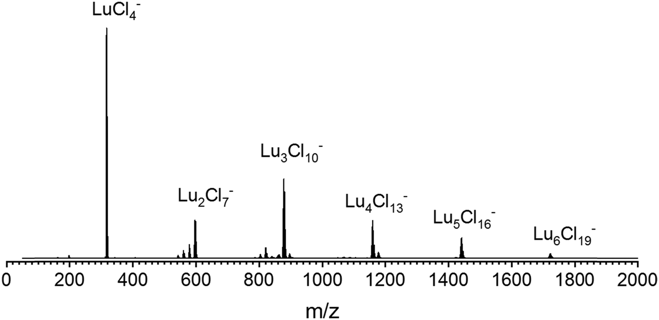

Fig. 1 An overview ESI mass spectrum of a solution of 0.05 mmol l⁻¹ LuCl₃ in isopropanol, negative mode. The small peaks in front of the Lu₂Cl₇⁻ and Lu₃Cl₁₀⁻ signals correspond to Lu₂Cl_7−x(OH)_x⁻ (x = 1–3) and Lu₃Cl_10−x(OH)_x⁻ (x = 1–4), respectively. The small peaks after Lu₃Cl₁₀⁻ and Lu₄Cl₁₃⁻ correspond to water adducts, i.e. Lu₃Cl₁₀(H₂O)⁻ and Lu₄Cl₁₃(H₂O)⁻, respectively. The other LnCl₃ solutions showed analogous overview mass spectra. The IMS measurements reported below were performed under mass-selective conditions, i.e. results are specific to Ln_xCl_3x+1⁻, x = 1–6, throughout (no contribution of –OH or H₂O adducts).

Solid LnCl₃ samples were obtained mostly as hydrate salts from commercial sources and were used without further purification: LaCl₃, HoCl₃, LuCl₃(H₂O)₆, and TmCl₃(H₂O)₆ from Sigma Aldrich, NdCl₃(H₂O)_x, SmCl₃(H₂O)_x, TbCl₃(H₂O)_x, and ErCl₃(H₂O)_x from Chempur, CeCl₃(H₂O)₇, DyCl₃(H₂O)₆, and GdCl₃(H₂O)₆ from Fluorchem, EuCl₃(H₂O)_x from Alfa Aesar and PrCl₃(H₂O)_x from Angene.

2.2 Ion mobility measurements

For subsequent ion mobility analysis, the respective cluster sizes were first isolated in the quadrupole mass filter prior to the ion mobility cell in order to exclude any contamination of the mobilograms of the smaller cluster sizes by possible fragmentations of larger species during the ion mobility measurement. Furthermore, the mobility analysis is performed only for a narrow mass window (depending on the isotope pattern of the respective Ln) selected using instrument software (MassLynxV4.2). The ion mobility measurement is performed in a cyclic ion mobility cell (cIM) combined with a pre-storage device. The effective drift length and accordingly the IMS resolution can be modified by adjusting the number of cycles. The resolution (and measurement time) increases with the number of cycles. The arrival time distributions after 10 cycles are shown in Fig. 2 for all Ln_xCl_3x+1⁻ studied. As a general trend (at a given x), we observe the peak arrival time decreasing almost linearly from La to Lu in line with the lanthanide contraction. There are however some exceptions: for Ln₄Cl₁₃⁻, we observe a strong decrease in the arrival time from La to Nd while from Sm to Lu, the arrival time is almost constant. For Ln₅Cl₁₆⁻, the arrival time decreases from La to Ce, as expected, but increases from Ce to Nd, and therefore Nd has the largest arrival time along the series. For all Ln_xCl_3x+1⁻ (x ≤ 5), we found a single, sharp peak in the arrival time distribution with the peak width corresponding to the instrumental resolution. For Ln₆Cl₁₉⁻, the arrival time distribution is bimodal for Ln = Sm–Lu, with the relative intensity of the first peak decreasing from 94% (Sm) to 30% (Lu).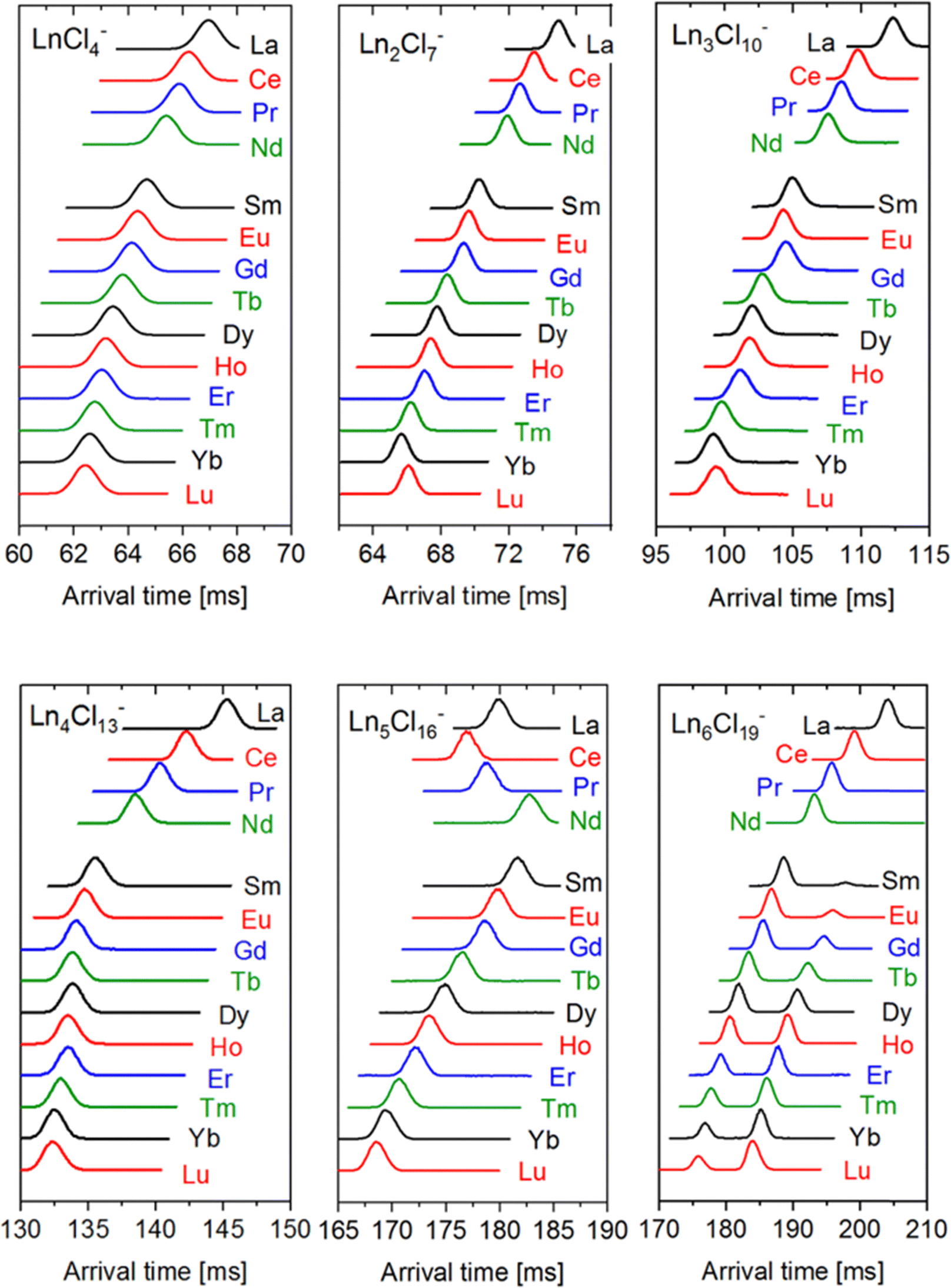

Fig. 2 Typical arrival time distributions of Ln_xCl_3x+1⁻ anions after 10 cycles (for given x =1–6 as indicated). A travelling wave (TW) speed of 375 m s⁻¹ was used in all cases. For x = 2–6, a TW height of 18 V was used. LnCl₄⁻ (x = 1) was measured with a TW height of 14 V (at 18 V the large mobility of this ion causes undesirable “surfing” on the TW rather than CCS dependent separation).

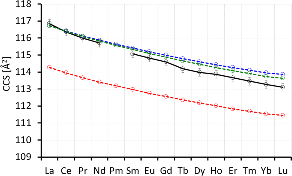
Arrival times depend on many instrumental parameters which need to be taken into account before comparing with predictions from theory. Furthermore, the arrival time of an ion consists of the time it needs to pass the cIM and the (mass-dependent) transfer time to the detector.¹⁰ We eliminate transfer time contributions by measuring the arrival time after typically 1, 5 and 10 cycles and determining the time-per-cycle by a linear fit of the arrival time vs. the number of cycles. This time still depends on many instrumental parameters such as buffer gas (nitrogen) pressure, temperature, speed and height of the travelling wave. In order to obtain a device-independent collision cross-section (^TWCCS_N2), we calibrate against the set of “Agilent tunemix” ions using the CCS values of Stow et al.¹² This calibration procedure is performed each day under exactly the same conditions as the mobility measurements of the lanthanide chloride clusters. All measurements were done at least in triplicate on different days. This workflow resulted in highly reproducible CCS values with statistical errors in most cases below 0.2%. The values are summarized in Table 1 and Fig. 3.

Table 1 Experimental travelling wave ^TWCCS_N2 values for Ln_xCl_3x+1⁻ anions (in Ų). For Ln₆Cl₁₉⁻ (Ln = Sm–Lu), we observe two peaks corresponding to two non-interconverting isomers. The relative intensities of the two isomers are given in brackets

	LnCl4^−	Ln2Cl7^−	Ln3Cl10^−	Ln4Cl13^−	Ln5Cl16^−	Ln6Cl19^−
La	116.8	150.3	176.5	196.6	216.0	228.7 (100%)
Ce	116.4	149.1	174.8	194.9	214.3	226.2 (100%)
Pr	116.0	148.3	173.8	193.6	215.3	224.4 (100%)
Nd	115.7	147.8	173.2	192.5	217.4	223.0 (100%)
Sm	115.1	146.3	171.5	190.7	216.8	220.5 (94%)	225.5 (6%)
Eu	114.8	145.8	170.9	190.2	215.7	219.5 (89%)	224.3 (11%)
Gd	114.6	145.5	171.0	189.7	215.1	218.8 (80%)	223.6 (20%)
Tb	114.2	144.7	169.8	189.6	214.0	217.6 (69%)	222.4 (31%)
Dy	114.0	144.1	169.2	189.6	213.0	216.7 (55%)	221.4 (45%)
Ho	113.9	143.8	169.0	189.4	212.3	215.9 (47%)	220.6 (53%)
Er	113.7	143.6	168.8	189.5	211.7	215.5 (42%)	220.1 (58%)
Tm	113.5	142.8	167.7	189.0	210.7	214.4 (38%)	219.0 (62%)
Yb	113.3	142.4	167.4	188.8	210.2	214.1 (33%)	218.7 (67%)
Lu	113.1	142.7	167.5	188.8	209.5	213.4 (30%)	217.8 (70%)

---

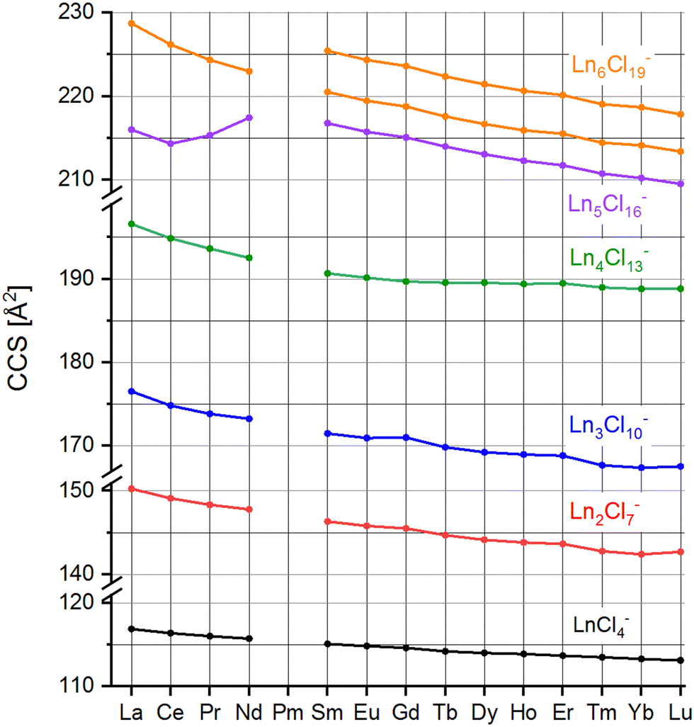Fig. 3 Collision cross-sections ^TWCCS_N2 of Ln_xCl_3x+1⁻, x = 1–6, Ln = La–Lu except Pm (see Table 1).

2.3 IMS–IMS experiment

The Ln₆Cl₁₉⁻ arrival times show a bimodal distribution for Sm–Lu, with the relative intensity of the second (larger CCS) peak increasing smoothly from 6% for Sm₆Cl₁₉⁻ to 70% for Lu₆Cl₁₉⁻. The question that arises is whether this is merely a consequence of the ionisation process (solvent, concentration, and source voltages), i.e. some kinetic trapping of the solution phase composition, or whether it reflects the thermodynamic stability of the two isomers in the gas phase. In a first step, we widely varied the source conditions (needle voltage: 2.5–4 kV and cone voltage: 40–80 V) but could not find a significant change in isomer compositions (within 5% relative intensity). A unique feature of the Waters cyclic instrument (among commercial systems) is the capability to perform IMS–IMS experiments with a collisional activation step between the first and second IMS step. The workflow for it is as follows: for the mass selected Ln₆Cl₁₉⁻, we first perform a five-cycle separation sequence (5 cycles are enough to baseline separate the two peaks). In a second step, we remove the ions corresponding to either the first or the second peak by switching the cIM at the appropriate time. The remaining ion packet is transferred into the pre-store (an ion trap located prior to the cIM).¹⁰ Third, these ions are reinjected into the cIM with an adjustable kinetic energy (0–100 eV, lab frame (against N₂ collision gas)) and cycled for another 5 cycles. The results are shown in Fig. 4a for Ho₆Cl₁₉⁻ as an example. When the first peak “isomer 1” is selected, then transferred into pre-store, reinjected with nominally 0 eV and separated for another 5 cycles, only the unchanged peak at 199 ms is observed, corresponding to the unchanged arrival time of isomer 1. When the injection energy is increased, a second peak at 203 ms appears that corresponds to isomer 2. Finally, at 60 eV, this second peak dominates. If the second peak (“isomer 2”, Fig. 4b) is isolated first and reinjected with 0 eV, only the peak at 203 ms corresponding to isomer 2 is observed. With increasing injection energy, the peak at 199 ms appears, corresponding to isomer 1. At 60 eV and above, we see the same intensity ratio, 35% of isomer 1 and 65% of isomer 2, independent of which isomer is selected in the first place (Fig. 4c). This is a clear indication that during the annealing step associated with reinjection, (i) ions become sufficiently excited to rapidly interconvert multiple times before (ii) cooling back down to room temperature on a timescale faster than one cIM cycle, i.e. there is no further interconversion in the cIM (otherwise we would observe a single peak at the weighted average of the two isomers, or at least a significant filling of the baseline in between the two peaks).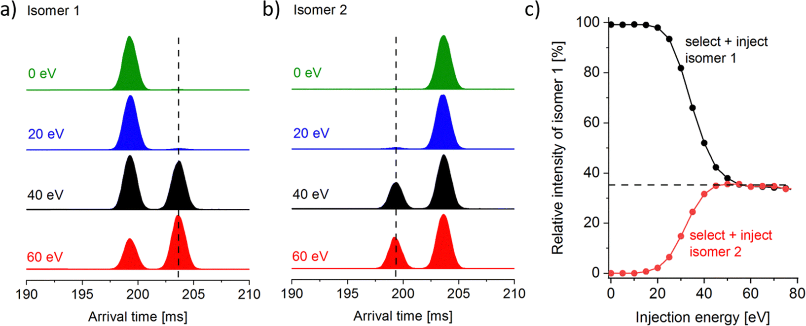

Fig. 4 IMS–IMS experiment for Ho₆Cl₁₉⁻. (a) The first peak of the arrival time distribution (isomer 1 shown after 5 cycle separation) is selected, transferred into the pre-store, reinjected with variable kinetic energy and separated for another 5 cycles. (b) The same workflow with the second peak selected (isomer 2). (c) The isomer distribution as a function of injection energy. It should be noted that this is the same for either prehistory (a) or (b).

For the other lanthanides (Sm–Lu), different equilibrium isomer ratios are observed, see Fig. 5. In all cases, the isomer ratio does not depend on the isomer that is selected and reinjected (Fig. 5, black and red data points). Across the lanthanide series, there is a clear trend: the relative intensity of isomer 1 decreases strongly from 70% for Sm to 21% for Lu. This parallels the observed intensity ratios observed by electrospraying the respective lanthanide chloride solution (and by measuring the “as-prepared” isomer composition with minimal injection energy (Fig. 5, green data points)).

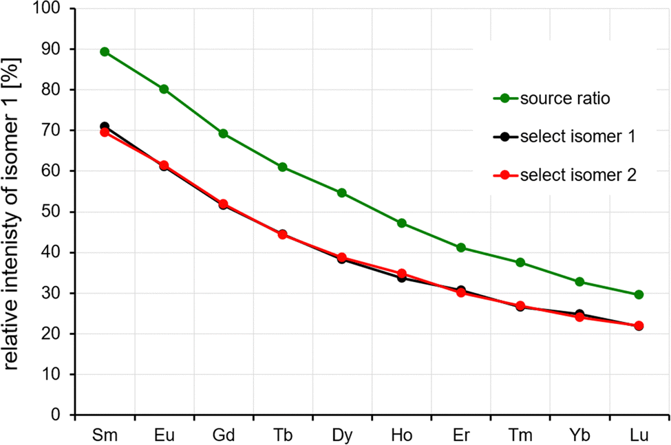Fig. 5 IMS–IMS experiment for Ln₆Cl₁₉⁻, Ln = Sm–Lu. The observed relative intensities at 50 eV reinjection energy are independent of the choice of the isomer stored and reinjected (red and black data points). For comparison, the isomer ratios observed directly from the source are shown as green data points. See the text.

However, the ratios are slightly different quantitatively, probably due to the fact that the two different experimental workflows are associated with different excitation, cooling and detection histories.

3. Theoretical methods and results

3.1 Quantum chemical calculations

The energy surfaces of Ln_xCl_3x+1⁻, Ln = La–Lu and x = 2–6, were investigated with TURBOMOLE¹³ in the following way. First, for each x and each Ln, a genetic algorithm procedure¹⁴ was carried out, scanning in total more than 5000 isomers for each Ln at the level PBE/lcecp-1-SVP, i.e. employing the PBE functional¹⁵ with def2-SVP bases¹⁶ for Cl; for lanthanides, large-core fⁿ⁻¹ effective core potentials^17,18 were employed (covering, e.g. for Pr, the inner shells plus two f electrons) together with newly designed error-balanced polarized double zeta basis sets⁹ lcecp-1-SVP. For a given x, the structure lowest in energy and all energetically following, up to ca. 100 kJ mol⁻¹, were collected for all Ln, and then redundant structures were removed. In this way, typically about three isomers for each size were obtained. These sets of structures were optimized for all Ln at the level PBE/lcecp-1-TZVP⁹ with fine grids (grid size 5¹⁹) and tight convergence (energy to 10⁻⁹E_h). The optimized structures were symmetrized to the highest symmetry, which in the case of imaginary frequencies was again lowered until their disappearance. For estimating the consistency with other methods, the resulting structures were additionally re-optimized at the level TPSS²⁰/lcecp-1-TZVP and for x = 2 additionally PBE0²¹/lcecp-1-TZVP and PBE0/lcecp-1-QZVP,⁹ and further with the all-electron scalar relativistic X2C method^22,23 with the PBE0 functional and x2c-TZVPall²⁴ as well as x2c-QZVPall²⁵ basis sets. Structure parameters for all these methods were compared for the monomer. Furthermore, for each species, vibrational spectra were calculated, which yielded real frequencies throughout and served for the free energy calculation within the harmonic oscillator rigid rotor model at 0, 300 and 600 K. Finally, transition pathways between the lowest and the second-lowest isomer were optimized with a generalized Newton-method²⁶ at the level PBE/lcecp-1-TZVP and the identified maxima were fine-optimized employing the corresponding tool in TURBOMOLE with default options.

3.2 Comparison of experimental and calculated CCS

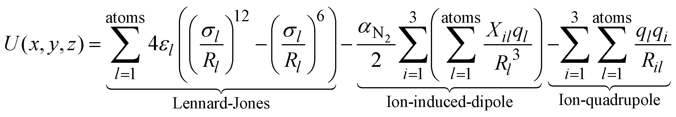
The experimental ^TWCCS_N2 can be used to rule out or confirm the quantum chemically determined candidate structures by comparison with calculated ^theoCCS_N2. This is done by trajectory method calculations as implemented in IMoS1.09.^27,28 The interaction potential between the drifting ion and a nitrogen buffer gas molecule is modelled (atom by atom) by a combination of Lennard-Jones, ion-induced dipole and ion-quadrupole interactions with the following assumptions: the Lennard-Jones parameters ε_l and σ_l are treated as element specific, the ion-induced dipole is modelled with the polarizability of nitrogen (α_N2) and the partial charges q_l (from ESP-fit) on each atom. For the ion-quadrupole interaction, the quadrupole moment of nitrogen is modelled by 3 partial charges q_i located at appropriate distances.²⁹
While for H, C, O, N and F the respective Lennard-Jones parameters have been optimized in IMoS using a test-set of small (covalently bound, organic) molecules;³⁰ for other elements, only the default values of ε = 2.6 meV and σ = 3.5 Å are implemented in IMoS. With these values, we obtain ^theoCCS_N2 that are ca. 7% too small; therefore, a further calibration process is needed. In test calculations, it turns out that the influence of σ_Ln on the calculated CCS is ca. ten-fold smaller than σ_Cl (see Fig. 6). We therefore opt to use the same values for all Ln while optimizing the parameters for Cl. ε_Cl and σ_Cl are correlated, i.e. several combinations thereof give similar CCS. In order to stick as close as possible to the IMoS default parameters, we have kept ε constant at its default value of 2.6 meV and have only adjusted σ_Cl.

Fig. 6 Experimental (black, with error bars; ^TWCCS_N2) and calculated CCS (red, blue, green; ^theoCCS_N2) for LnCl₄⁻. Red: IMoS-parameters σ_Cl = 3.85 Å and (constant) σ_Ln = 3.00 Å, blue: σ_Cl = 3.95 Å and (constant) σ_Ln = 3.00 Å, green: σ_Cl = 3.95 Å and σ_Ln linearly decreasing from 3.00 Å for La to 2.8 Å for Lu. It should be noted that σ_Ln has comparatively little influence on ^theoCCS_N2 of the monomers because the collision gas scatters from the enclosing chloride shell.

In the following, we have used our ^TWCCS_N2 values for LaCl₄⁻, La₃Cl₁₀⁻, La₄Cl₁₃⁻ and La₆Cl₁₉⁻ as calibration points to iteratively find an optimal value for σ_Cl because, based on the DFT calculations (see Section 3.1 and also below), there is little doubt about the respective energetically favored structures: LaCl₄⁻ is a tetrahedron, La₃Cl₁₀⁻ and La₄Cl₁₃⁻ are ring structures and La₆C₁₉⁻ is an octahedron; other isomers are energetically significantly less favorable. The tabulated ionic radii of Cl⁻, La³⁺ and Lu³⁺ (in coordination number 6) are 1.81 Å, 1.032 Å and 0.861 Å,³¹ respectively, i.e. on average the Ln³⁺ ion is expected to be 0.8–0.9 Å smaller than the Cl⁻ ion. Keeping this difference in mind we find for σ_Cl = 3.87 Å and σ_La = 3.00 Å a close fit (within 1%) between the experimental (196.6 Ų) and calculated (195.0 Ų) CCS of La₄Cl₁₃⁻. If we calculate ^theoCCS_N2 of monomer LaCl₄⁻ with these parameters, we find that it is 1.9% below the experimental value (114.5 Ųvs. 116.8 Ų). For the trimer La₃Cl₁₀⁻, the deviation is −1.4%. For the hexamer La₆Cl₁₉⁻, the order is reversed, and the theoretical CCS is 2.1% larger than the experimental value (233.4 Ųvs. 228.7 Ų). While a deviation of 2–3% is not uncommon for CCS calculations based on DFT-optimized structures, a better fit for the four calibration points would be desirable. However, with just element-specific parameters, we clearly cannot achieve a perfect fit for all four calibration points simultaneously: if we adjust parameters to perfectly match the theoretical and experimental CCS of La₄Cl₁₃⁻, LaCl₄⁻ is always slightly (ca. 2%) too small while La₆Cl₁₉⁻ is slightly (ca. 2%) too large (see Fig. S1, ESI† for plots of ^theoCCS_N2 as a function of σ_Cl). The problem most likely arises from the use of element specific, but charge-independent L-J parameters in IMoS. This is more critical in highly polar systems like the clusters considered here: the overall charge per atom is larger in the smaller ions like LaCl₄⁻ and therefore their effective van der Waals radii are larger. Rather than taking the somewhat questionable step of also adjusting this parameter for each cluster size we decided to keep the σ_Cl constant at 3.87 Å (a value which minimizes the overall error) unless otherwise noted. Therefore, for the following, we have to keep in mind that with this parameter choice, the ^theoCCS_N2 of the smaller cluster sizes will be slightly underestimated and the larger cluster sizes will be slightly overestimated.

4. Discussion

Next, we discuss the inferences which can be made by comparing ^TWCCS_N2 with DFT derived model structures (following the procedure described in the previous section) in order of increasing oligomer size.

4.1 Calculated structures and CCS

LnCl₄⁻. According to our DFT calculations, isolated LnCl₄⁻ is tetrahedral with Ln–Cl distances ranging from 2.674 Å (La) to 2.483 Å (Lu). Differences in values obtained with larger bases, other functionals and all-electron relativistic X2C treatments are very systematic, see Fig. S3 (ESI†), and may be summarized as follows: d(TZVP) = d(QZVP) − 0.3 pm, d(PBE) = d(PBE0) + 0.8 pm = d(TPSS) − 0.8 pm, and d(ECP) = d(X2C) + 2.1 pm. This slight overestimation when using ECPs instead of all-electron relativistic methods is also visible from the comparison with the numbers obtained by Rutkowski et al.⁸ in their all-electron (ZORA) DFT calculations for La and Lu, 2.669 Å and 2.467 Å, respectively. Our experimental ^TWCCS_N2 values decrease monotonically from 116.8 Ų for LaCl₄⁻ to 113.1 Ų for LuCl₄⁻. This overall trend of decreasing CCS is reproduced in the DFT + trajectory calculations: ^theoCCS_N2 (calculated with σ_Cl = 3.87 Å and σ_Ln = 3.00 Å for all Ln) ranges from 114.5 Ų to 112.0 Ų, see Fig. 6 (red line and symbols). As discussed in the previous section, these values are systematically slightly (ca. 1–2%) smaller than the experimental values. If we adjust σ_Cl to 3.96 Å in order to match the experimental CCS for LaCl₄⁻, we in turn slightly overestimate the CCS for LuCl₄⁻ (calcd: 113.9 Ųvs. exp. 113.1 Ų; Fig. 6, blue line and symbols), i.e. we can reproduce the experimental trend qualitatively, but not perfectly. If we furthermore decrease σ_Ln linearly from 3.0 Å for Ln = La to 2.8 Å for Ln = Lu, in line with the tabulated ionic radius decrease due to lanthanide contraction, we obtain almost the same values (Fig. 6, green line and symbols). This shows that the van der Waals radius σ_Ln of the lanthanide that is used in the IMoS calculation has basically no effect on the calculated CCS. This is not unexpected since the central atom is surrounded by a shell of chlorine atoms i.e. the buffer gas scatters mostly from the chlorine atoms and not from the lanthanide – thus supporting our decision to use the same radius for all lanthanides in the following. With these parameter choices, we can reproduce the experimental trend of decreasing CCS from La to Lu to within 1% for all LnCl₄⁻.

Ln₂Cl₇⁻. For the dimer Ln₂Cl₇⁻, the experimental ^TWCCS_N2 values decrease from 150.3 Ų to 142.7 Ų. In the calculations, we find two isomers within 10 kJ mol⁻¹ of each other for all Ln: in isomer A with C₁ symmetry, three chlorine atoms bridge the lanthanides while isomer B (C_s symmetry) has two bridging chlorine atoms (Fig. 7). A third isomer (C, with C_3v symmetry) with the lanthanide coordinated to 4 and 6 chlorine atoms, respectively, is more than 25 kJ mol⁻¹ higher in energy. Of note is that for simplicity we here discuss only the electronic energies at the PBE/lcecp-1-TZVP level. Differences in other methods of calculation are systematic and may be summarized as follows (for both minima and barriers). Changes when using X2C instead of ECPs amount to ∼5 kJ mol⁻¹, which is in the range of those when using different functionals (PBE/PBE0/TPSS) or that of considering ΔG(300 K) instead of ΔE; the difference between TZVP and QZVP bases is ∼1 kJ mol⁻¹; all these data for all lanthanides are displayed in Tables S1 and S2 (ESI†) as well as Fig. S4 and S5 (ESI†). Therefore, the disfavoring of isomer C by more than 25 kJ mol⁻¹ is significant; it cannot be expected to contribute significantly to an equilibrium distribution and is thus ruled out. For the early lanthanides, isomer A is significantly lower in energy than isomer B; for the later lanthanides, both isomers become close in energy and finally their energy ordering inverts. It should be noted that this finding is in line with the DFT calculations of Rutkowksi et al.⁸ who found isomer A for La₂Cl₇⁻ and isomer B for Lu₂Cl₇⁻. The calculated ^theoCCS_N2 value of isomer A ranges from 146.7 Ų (La) to 139.8 Ų (Lu), i.e. they are 2.5% to 2.0% smaller than the experimental values – somewhat more than the ca. 1–2% difference we expect for the small cluster sizes (see above, LnCl₄⁻). For isomer B, the ^theoCCS_N2 value ranges from 152.1 Ų to 145.3 Ų, 1–2% larger than the experimental value. For a given Ln, isomers A and B are predicted to differ from each other in CCS by ca. 3.5–4% which should be easily resolvable in our experiment if both were simultaneously present in significant amounts and non-interconverting. However, we observe in all cases only one narrow peak (with a peak width corresponding to an experimental resolution of >200) pretty much between that expected for A and B. This finding can be explained by an equilibrium and a quick interconversion between the two isomers A and B, which is much faster than the experimental time scale (ca. 6–7 milliseconds per cycle). Based on the DFT calculation, the barrier between isomers A and B is only between 6 and 16 kJ mol⁻¹ (relative to isomer A). Therefore, we conclude that in our ion mobility experiment we most likely observe an interconverting mixture of isomers A and B. For an arrival time simulation of interconverting isomers, see Fig. S2 (ESI†).

Fig. 7 Left: Experimental ^TWCCS_N2 (black) with error bars and calculated ^theoCCS_N2 (red, blue) for the two lowest energy isomers of Ln₂Cl₇⁻. IMoS-parameters σ_Cl = 3.85 Å and σ_Ln = 3.00 Å. Right: Calculated energy of isomer B with respect to isomer A (ΔE, no ZPE correction).

Ln₃Cl₁₀⁻. For the trimer Ln₃Cl₁₀⁻, the experimental ^TWCCS_N2 value decreases from 176.5 Ų to 167.5 Ų. In the lowest energy isomer that we obtained consistently for all lanthanides (isomer A, C_2v symmetry, the structure that has also been found for La₃Cl₁₀⁻ and Lu₃Cl₁₀⁻ by Rutkowski et al.⁸), the lanthanide atoms form a triangle where each edge is bridged by one chlorine atom, and two additional chlorine atoms are located centrally above and below the triangular plane. Isomer B with C_3v symmetry is a variant of this structure with one central chlorine atom and each Ln atom further having two terminal Cl atoms. It is 15–18 kJ mol⁻¹ higher in energy than isomer A. The chain-type isomer C, 21–27 kJ mol⁻¹ higher in energy than A, corresponds to a consistent structural extension of the most stable isomer for Ln₂Cl₇⁻ (see Table S4 and Fig. S6, ESI†). Based on the relative energies, this isomer can be excluded.

The ^theoCCS_N2 value for isomer A is in the range of 174.2–164.0 Ų, i.e. 1.0–2.1% below the experimental value and that for isomer B is 2.9–4.9% above, see Fig. 8. The linear chain, isomer C, is between 1.0% and 2.1% above the experimental value. Among the three possibilities, isomer A is in best agreement with the experiment, especially as we expect the CCS calculated for smaller clusters like Ln₃Cl₁₀⁻ to be slightly below the experimental value (based on our calibration procedure, see above). Isomer interconversion on the experimental timescale does not need to be invoked here. The closest higher lying isomers are uniformly 15–18 kJ mol⁻¹ less favorable and would therefore not be expected to contribute significantly to a room temperature equilibrium distribution.

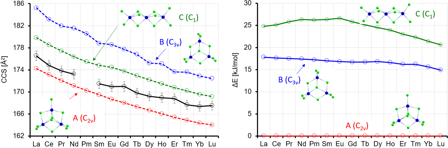Fig. 8 Left: Experimental (black) with error bars and calculated CCS (red, blue, green) for Ln₃Cl₁₀⁻. Right: Calculated energy differences (with respect to isomer A) (ΔE, no ZPE correction).

Ln₄Cl₁₃⁻. The trend of experimental ^TWCCS_N2 values vs. the Ln element observed for the tetramers differs qualitatively from that observed for the smaller clusters. After a steep decrease for the early lanthanides (La – 196.6 Ų to Gd – 189.7 Ų), the CCS-decrease is much smaller for the late lanthanides (Gd – 189.7 Ų to Lu 188.8 Ų).

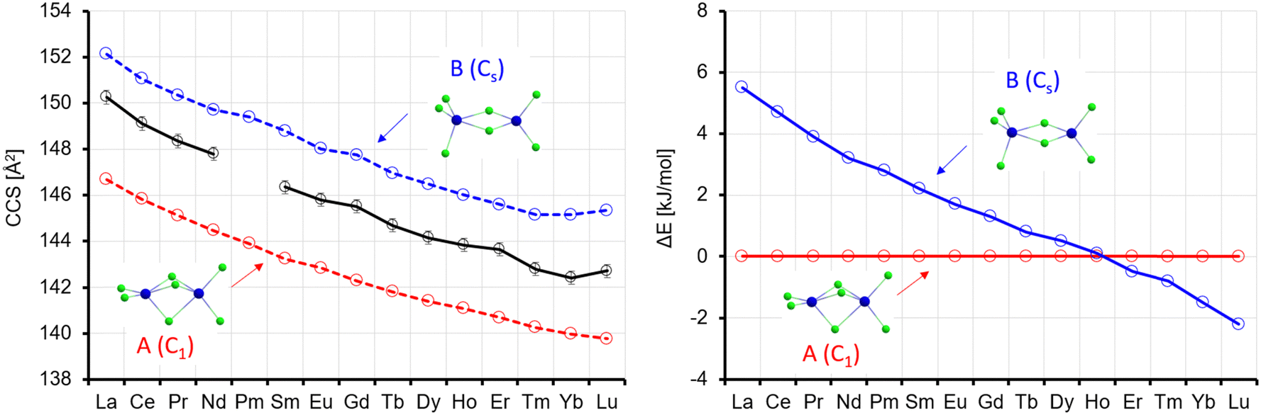
In the lowest energy isomer A for La₄Cl₁₃⁻, the four Ln atoms form a square with two bridging Cl atoms on each edge. Each Ln atom has a terminal Cl atom, and the last Cl atom is in the centre. For La, this isomer is preferred by 16 kJ mol⁻¹ over B, where the Ln atoms form a butterfly structure, with edges and planes bridged by Cl, and additionally two terminal Cl each at two of the Ln atoms and one each at the two others. The preference for A continuously decreases, and from the element Tb onwards isomer B is preferred (by up to 12 kJ mol⁻¹ for Lu, see Fig. 9). It should be noted that Rutkowski et al. found isomer A for both La₄Cl₁₃⁻ and Lu₄Cl₁₃⁻. Other isomers are more than 50 kJ mol⁻¹ higher in energy and can be ruled out (see Table S5 and Fig. S7, ESI†). The ^theoCCS_N2-curve for A (Fig. 9, red curve) has a basically constant slope and closely follows the experimental CCS curve from La to Gd. The ^theoCCS_N2 curve of B (Fig. 9, left, blue curve) parallels the curve of A (but shifted to larger CCS by 5–7 Ų). It meets the experimental data in the range from Tm to Lu. This suggests that a structural transition from isomer A to isomer B occurs along the series, which is perfectly in line with the predicted relative energies: the energy difference between isomer B and isomer A decreases from La to Gd and for Tb–Lu isomer B becomes favored (Fig. 9, right).

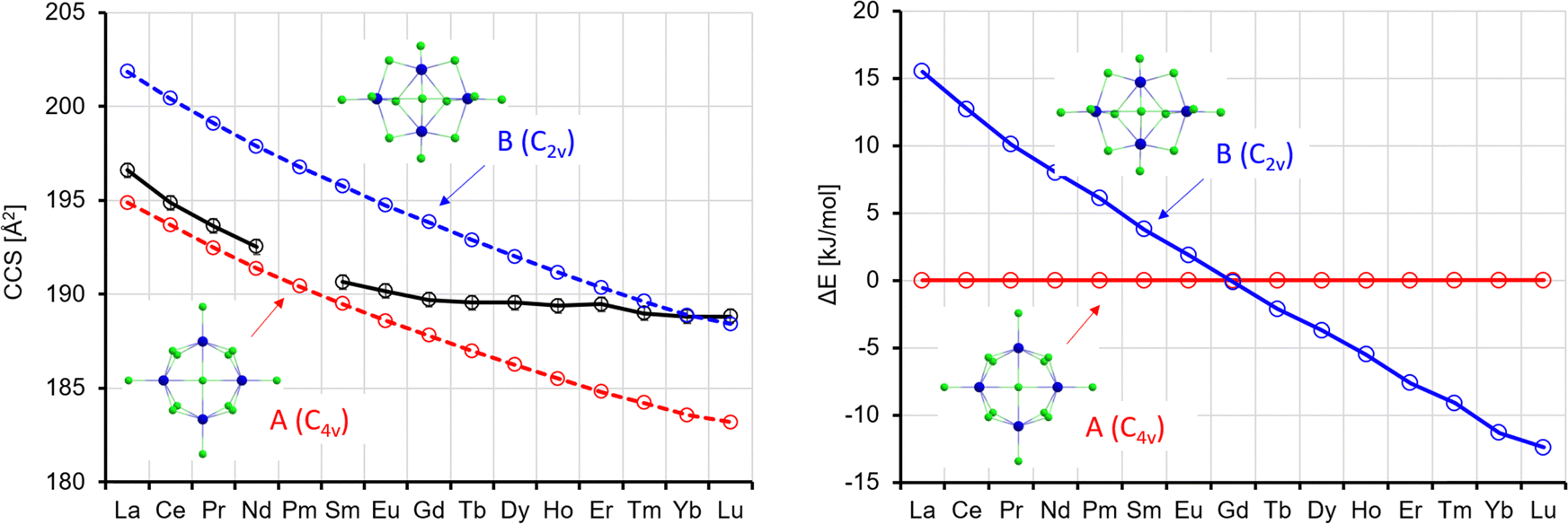Fig. 9 Left: Experimental (black) with error bars and calculated CCS (red, blue) for Ln₄Cl₁₃⁻. Right: Calculated energy differences (with respect to isomer 1); ΔE, no ZPE correction.

It is interesting to note that we always observe only one sharp peak in the arrival time distribution (see Fig. 2), even in the intermediate region from Eu to Tm. This can most likely be explained by a quick interconversion between the two isomers in this region (the barrier height is ca. 60 kJ mol⁻¹, see Table S8, ESI†). This leads to an averaged collision cross-section which is weighted by the relative amounts of isomers A and B in the Ln-dependent equilibrium distributions (in turn reflecting free energy differences which correlate with ΔE's as shown in Fig. 9).³²

Ln₅Cl₁₆⁻. The experimental ^TWCCS_N2vs. the Ln plot for the pentamers differs drastically from the curves of the smaller clusters (see Fig. 10, black): first, from La to Ce, the ^TWCCS_N2 values decrease as expected (La₅Cl₁₆⁻: 216.0 Ų to Ce₅Cl₁₆⁻: 214.3 Ų), but between Ce and Nd the ^TWCCS_N2 value increases again (Pr₅Cl₁₆⁻: 215.3 Ų, Nd₅Cl₁₆⁻: 217.4 Ų). Thereafter, from Sm to Lu, we observe an expected monotonic decrease (Sm₅Cl₁₆⁻: 216.8 Ų to Lu₅Cl₁₆⁻: 209.5 Ų).

Fig. 10 Left: Experimental (black) with error bars and calculated CCS (red, blue, green) for Ln₅Cl₁₆⁻. Right: Calculated energy differences (with respect to isomer 1) (ΔE, no ZPE correction).

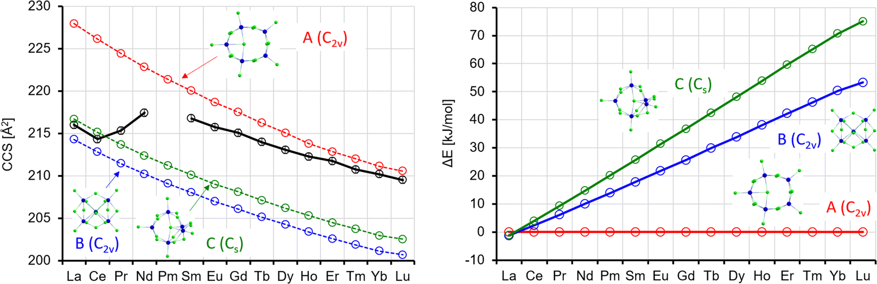
According to the calculations, the lowest energy isomer A shows C_5v symmetry, from Ho to Lu and thus is a straightforward structural extension of the most stable isomer for x = 4. For the lighter lanthanides, it is slightly distorted to C_2v (in-line with the calculations of Rutkowski et al.,⁸ who considered this isomer only for La and Lu). Also, isomer C is a ring-type isomer, but here only three atoms reside in the plane. At the last corner of an imaginary square, there is one Ln atom above and one below the plane. For the remainder, the Cl bridges are similar to isomer A, and, like there, one Cl is in the middle of the ring. Isomer B may be regarded as the next step in this structural development. One corner of an imaginary triangle is occupied with one Ln atom, the two others each with one Ln atom above and one below the plane. In total, there are ten bridging Cl atoms, further one terminal Cl per Ln, and one Cl in the middle. Whereas for La, isomers A–C are practically degenerate, B and C become progressively less favourable across the Ln series to reach 53(71) kJ mol⁻¹ for B(C) at Lu (see also Table S6 and Fig. S8, ESI†).

The ^theoCCS_N2 for isomer A closely matches the experimental ^TWCCS_N2 for Sm–Lu (see Fig. 10). For La and Ce, however it is much (>5%) larger than the experimental values and can therefore be ruled out in the experiment. On the other hand, the quasi-degenerate isomers B and C match the experimental CCS almost perfectly (within 1%) in this region (see Fig. 10, left). So, from the experimental point of view, it is clear that isomers B and/or C are dominant for La (unlike the prediction by Rutkowski et al.⁸) and Ce, while isomer A dominates for Sm–Lu. This is in line with the relative energies: for the early lanthanides, all three isomers are close in energy (within 10 kJ mol⁻¹ or lower); for the late lanthanides, isomer A is strongly favored (by >30 kJ mol⁻¹, see Fig. 10, right). For the intermediate region (Pr and Nd), the situation is less clear: the experimental CCS are in between the calculations for isomers A, B, and C. On the other hand, the arrival time distributions for Pr and Nd are not significantly broader than the curves for the other lanthanides (Fig. 2) – we observe only one narrow peak. Therefore, we conclude that we observe a dynamical interconversion in this region, similar to what we have inferred for the intermediate region of Ln₄Cl₁₃⁻ (the barrier height is again ca. 60 kJ mol⁻¹, see Table S9, ESI†).

Ln₆Cl₁₉⁻. For the hexamer, we observe arrival time distributions with a single peak from La to Sm and bimodal distributions from Sm to Lu. For Sm, the first peak dominates, while for Lu the second peak is stronger in intensity (see Fig. 2). The corresponding ^TWCC_N2 are shown in Fig. 11 (black).

Fig. 11 Left: Experimental (black) with error bars and calculated CCS (red, blue, green) for Ln₆Cl₁₉⁻. Right: Calculated energy differences (with respect to isomer 1) (ΔE, no ZPE correction).

In the O_h-symmetric isomer A, the Ln atoms form an octahedron, whose edges are bridged by two Cl atoms each. Each Ln has one terminal Cl, and one Cl resides in the centre. In C_3v-symmetric B, all corners of an imaginary triangle are occupied each with one Ln atom above and one below the plane; it is thus closely related to isomer B for x = 5, also concerning the positions of the Cl atoms. C is a Cl double-bridged six-membered Ln ring with one more terminal Cl at five of the Ln atoms. At the sixth Ln atom, the ring is bent inwards. There is no terminal Cl here; instead, there are two Cl inside the ring. For La, B(C) is higher in energy by 21(34) kJ mol⁻¹ (see Table S7 and Fig. S9, ESI†). Whereas the energetic disfavouring of C increases somewhat towards Lu, it decreases for B. If we compare the calculated CCS for isomer A (La: 233.9 Ų, using the “standard” σ_Cl value of 3.85 Å, see above), it is the isomer that fits best (within ca. 2%) to the experiment (228.7 Ų) for La. Isomers B and C overestimate the CCS by ca. 4 and 11%, respectively, and it is clear that the single peak in the arrival time distribution of La₆Cl₁₉⁻ corresponds to isomer A. For the other lanthanides, isomer A parallels the experimental curve, and it is always ca. 2–3% too large (see Fig. 11, left, red and lower black curve). Isomer B corresponds to the second peak that we observe in the arrival time distribution of Ln₆Cl₁₉⁻ for Ln = Sm–Lu (see Fig. 2). Again, its CCS is ca. 2% larger than the experiment (Fig. 11, left, blue and upper black curve). Furthermore, the intensity increase of the second peak is in line with the decrease of energetic disfavoring of B (vs. A). Isomer C can be clearly ruled out both on the basis of relative energy and CCS. Rutkowski et al.⁸ predicted for La₆Cl₁₉⁻ a ring of 5 La atoms with a La atoms in the center and for Lu₆Cl₁₉⁻ a Lu-6-ring with a central Cl atom. These structures are more than 50 kJ mol⁻¹ above isomer A and can be ruled out. Note that the calculated barrier height between A and B is in the range of 100 kJ mol⁻¹ (Sm) to 130 kJ mol⁻¹ (Lu), see Table S8 (ESI†).

At this point, we should remind the reader that our calculations are performed at 0 K and do not include zero-point energy (ZPE), while the experimental arrival time distributions are determined in a measurement that is performed on cluster anions that are thermalized to near room temperature. Since we experimentally observe two base-line separated peaks in this measurement, it is clear that there is no significant interconversion on the experimental time-scale (10–100 ms) of the CCS determination. Therefore, the relative intensities of the two peaks as determined for the as-prepared clusters must reflect an elevated temperature, that is accessed somewhere upstream from the cIM for long enough to approach an equilibrium ratio (perhaps in the ESI† source or in the Stepwave ion guide). Clusters at this elevated temperature then quickly cool at latest after injection into the cIM cell.

We observe a decrease in the relative intensity of the first isomer in the arrival time distribution (experimental: isomer 1, calculation: isomer A) decreasing from 90 to 70% for Sm to 20–30% for Lu (depending on whether the ion intensities are measured directly by IMS or in IMS-selection-activation-IMS mode, see above, Fig. 5). In order to compare experiment and theory, we determined the equilibrium constants and relative ion intensities as a function of temperature (i.e. from relative free energies) expected for DFT-calculated relative energies, rotational constants and vibrational frequencies. The results are shown in Table 2 and Fig. 12. It turns out that isomer B is favored entropically for all Ln₆Cl₁₉⁻ and should therefore dominate the distribution at room temperature for Ho–Lu, which is very close to our experimental findings. It should be noted, however, that the predicted intensities are very sensitive to the parameters used in the calculation such as temperature, vibrational frequencies and relative energies, so the agreement might be fortuitous. For comparison, we include in the ESI† the relative energies obtained with TPSS and PBE0 functionals. The values are similar but they differ by 2–3 kJ mol⁻¹ with respect to the PBE values – which is enough to shift the intensity ratio significantly.

Table 2 Relative intensities of Ln₆Cl₁₉⁻ isomer A based on calculated energies, rotational constants and vibrational frequencies (for both isomers A and B). Vibrational frequencies are unscaled

Temperature [K]	La	Ce	Pr	Nd	Pm	Sm	Eu	Gd	Tb	Dy	Ho	Er	Tm	Yb	Lu
100	100	100	100	100	100	100	100	100	100	100	100	100	100	100	100
200	100	100	100	100	100	99	99	98	97	95	93	89	84	75	66
300	94	91	90	89	87	83	79	72	65	60	53	45	40	31	26
400	65	57	56	55	53	49	43	37	32	29	25	21	19	15	13
500	34	28	28	29	28	26	23	20	17	16	14	12	11	9	8

---

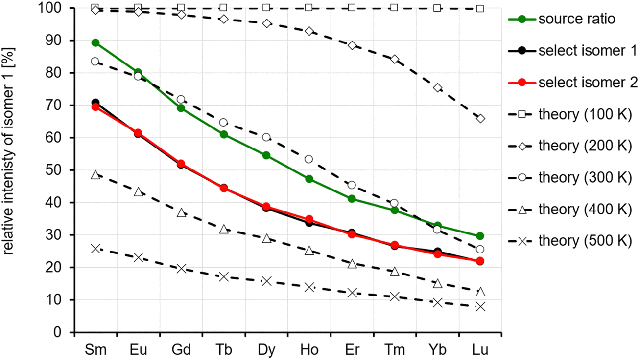Fig. 12 Comparison of observed ion intensities of the first isomer in the arrival time distribution (assigned as isomer A) with predictions based on DFT calculated relative energies, rotational constants and vibrational frequencies.

Conclusions

We have characterized the structures and isomer distributions of isolated Ln_xCl_3x+1⁻, x = 1–6, for all Ln = La–Lu (except Pm). Clusters were generated by ESI from isopropanol solutions. Based on observed concentration dependencies, they are likely being formed during the spray process itself rather than being present in solution. To probe Ln-dependent structural characteristics of these clusters, we have used cyclic IMS which can determine CCS to high precision (better than 0.2%) and resolution (significantly better than 200) by probing near room temperature ion ensembles during measurement times which range from 10 to 100 ms in length. In some cases, we have also used IMS–IMS to study isomer interconversion. Comparison of experimental results to comprehensive DFT calculations across the complete Ln series together with trajectory method modelling of the observed collision cross sections allows the studied anions to be categorized into two groups:

(a) those showing interconversion between two or more isomeric structures on a much faster than the experimental timescale (Ln₂Cl₇⁻, Ln₄Cl₁₃⁻ (Gd–Tm) and Ln₅Cl₁₆⁻ (Pr and Nd)) thus yielding an averaged CCS value and

(b) structurally rigid species which do not show significant isomeric interconversion during the measurement. Of special interest in this regard is the Ln₆Cl₁₉⁻ system. For Sm–Lu, two baseline separable isomers are observed whose relative ratios are strongly dependent on Ln. While they are rigid on a 100 ms timescale, each of these two isomers can be converted to the other structure by moderate collisional excitation – at energies still well below that required for dissociation. The Ln-dependent isomer ratios observed correlate with the equilibrium ratios predicted from DFT based relative free energies calculated for the two lowest energy Ln₆Cl₁₉⁻ structures.

For all Ln_xCl_3x+1⁻ studied, measurements are consistent with the lowest energy structures predicted in DFT calculations. In fact, where measurement and structural rearrangement timescales allow, we obtain an almost quantitative agreement between experiment and theory thus confirming isomer predictions and reproducing isomer intensity ratios.

Overall, the structures of Ln_xCl_3x+1⁻ reflect strong ionic bonding with limited directionality. They comprise Ln(III) centres bridged (and sometimes terminated) by multiple chlorides. This gives rise to ring and chain motifs for smaller clusters while for larger clusters more compact three-dimensional structures become favourable. At cluster sizes with two or more close lying isomers, the lanthanide contraction can lead to changes in structure types across the series. Interestingly, there is a condensed phase analogue to the O_h isomer A of Ln₆Cl₁₉⁻: W. P. Kretschmer et al. have reported the crystal structure of [Cp₆Yb₆Cl₁₃]⁻ with 6 terminating Cp rings instead of chlorides as in our case (and [Cp₃Yb₃Cl₅(thf)₃]⁺ counterions).³³ It is also instructive to consider how the gas-phase cluster structures can be related to each other in terms of a hypothetical assembly sequence involving sequential addition of LnCl₃⁻ units (bearing in mind that our experiments are consistent with the formation of thermodynamically favored isomeric structures even though the clusters must be growing in the presence of solvent molecules). This is shown in Fig. 13 which also summarizes the results from theory (structures and relative energies) for all species/cluster sizes.

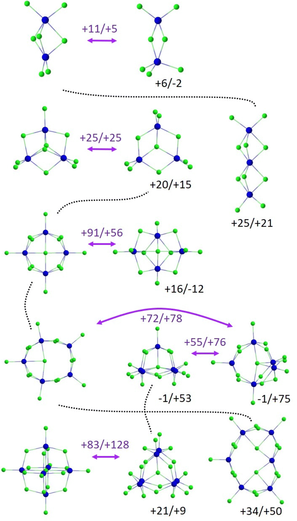Fig. 13 Energetically most favourable isomers of Ln_xCl_3x+1⁻ for each x and energy differences relative to isomer A (left) for La/Lu in kJ mol⁻¹. Straight purple arrows show calculated transitions within a given x and the energies for the optimized transition states for La/Lu relative to isomer A. Dotted lines indicate structural relationships between clusters of sizes x and x + 1 (via addition/insertion of LnCl₃⁻ units). The ESI† contains the top and side views of all structures shown.

We have begun to computationally address the daunting problem of multidimensional barrier surfaces and associated interconversion pathways (see Fig. S10–S13, ESI†). It would clearly also be interesting to experimentally study the T-dependence of isomer interconversion (on a different instrumental platform), e.g. to make interconversion slower by cooling the ion ensemble down sufficiently and thus to hopefully resolve the contributing isomers. Similar experiments with ESI sprayed ions in a T-variable drift cell have recently been performed by one of the groups contributing to this study.⁶ Along the same lines, we expect that interconversion of Ln₆Cl₁₉⁻ isomers A and B should become measurable by moderate heating.

A further direction for future work will be to extend this study to other lanthanide halides. For example, preliminary measurements on the Ln₆Br₁₉⁻ system indicates analogous isomerism but interestingly the interconversion becomes fast enough to cause broadening along the lines of the ATD's observed in ref. 4. Such data would allow fits of the interconversion kinetics to yield forward and reverse reaction rates (perhaps even as a function of Ln). This could be modelled by statistical rate theory to obtain effective activation energies which could be compared with DFT prediction.

Data availability

Most of the experimental data have been reported in the main text. Details of the collision cross-section and quantum chemical calculations including employed basis sets as well as coordinates and vibrational frequencies of the relevant species have been included as part of the ESI† (as separate files).

Conflicts of interest

There are no conflicts of interest to declare.

Acknowledgements

MK, FW, ML and PW gratefully acknowledge support from the German Science Foundation (DFG) as administered by the Collaborative Research Center 1573 “4f-for-future” in projects A2, C3 and Q. MK and PW are also grateful to DFG and KIT for the funding of a Cyclic IMS–MS instrument under Art. 91b GG. YN acknowledges funding of a six-month research stay in Karlsruhe by “GP-Chem” the International Joint Program in Integrated Chemistry of Tohoku University.

References

1. J. J. Berzelius, Om sammansättningen af vinsyra och drufsyra (John's säure aus den Voghesen), om blyoxidens atomvigt, samt allmänna anmärkningar om sådana kroppar som hafva lika sammansättning, men skiljaktiga egenskaper, Kungliga Svenska vetenskapsacademiens Handling (Transactions of the Royal Swedish Science Academy), 1840, vol. 49.
2. I. Gatland, Case Stud. At. Phys., 1974, 4, 369–437.
3. R. R. Hudgins, P. Dugourd, J. M. Tenenbaum and M. F. Jarrold, Structural transitions in sodium chloride nanocrystals, Phys. Rev. Lett., 1997, 78, 4213–4216.
4. P. Weis, T. Bierweiler, E. Vollmer and M. M. Kappes, Au₉⁺: Rapid isomerization reactions at 140 K, J. Chem. Phys., 2002, 117, 9293–9297.
5. S. Poyer, C. Comby-Zerbino, C. M. Choi, L. MacAleese, C. Deo, N. Bogliotti, J. Xie, J. Y. Salpin, P. Dugourd and F. Chirot, Conformational Dynamics in Ion Mobility Data, Anal. Chem., 2017, 89, 4230–4237.
6. R. Ito, X. He, K. Ohshimo and F. Misaizu, Large Conformational Change in the Isomerization of Flexible Crown Ether Observed at Low Temperature, J. Phys. Chem. A, 2022, 126, 4359–4366.
7. P. X. Rutkowski, M. C. Michelini, T. H. Bray, N. Russo, J. Marçalo and J. K. Gibson, Hydration of gas-phase ytterbium ion complexes studied by experiment and theory, Theor. Chem. Acc., 2011, 129, 575–592.
8. P. X. Rutkowski, M. C. Michelini and J. K. Gibson, Gas-phase lanthanide chloride clusters: relationships among ESI abundances and DFT structures and energetics, Phys. Chem. Chem. Phys., 2012, 14, 1965–1977.
9. M. Lukanowski and F. Weigend, manuscript in preparation; the lcecp-1-TZVP bases are provided within the ESI† as separate file.
10. K. Giles, J. Ujma, J. Wildgoose, S. Pringle, K. Richardson, D. Langridge and M. Green, A Cyclic Ion Mobility-Mass Spectrometry System, Anal. Chem., 2019, 91, 8564–8573.
11. F. Hennrich, S. Ito, P. Weis, M. Neumaier, S. Takano, T. Tsukuda and M. M. Kappes, Cyclic ion mobility of doped [MAu₂₄L₁₈]²⁻ superatoms and their fragments (M = Ni, Pd and Pt; L = alkynyl), Phys. Chem. Chem. Phys., 2024, 26, 8408–8418.
12. S. M. Stow, T. J. Causon, X. Y. Zheng, R. T. Kurulugama, T. Mairinger, J. C. May, E. E. Rennie, E. S. Baker, R. D. Smith, J. A. McLean, S. Hann and J. C. Fjeldsted, An Interlaboratory Evaluation of Drift Tube Ion Mobility-Mass Spectrometry Collision Cross Section Measurements, Anal. Chem., 2017, 89, 9048–9055.
13. Turbomole, Version 7.8 2023; a development of University of Karlsruhe and Forschungszentrum Karlsruhe GmbH 1989–2007, Turbomole GmbH, since 2007; available viahttps://www.turbomole.org.
14. M. Sierka, J. Döbler, J. Sauer, G. Santambrogio, M. Brümmer, L. Wöste, E. Janssens, G. Meijer and K. R. Asmis, Unexpected structures of aluminum oxide clusters in the gas phase, Angew. Chem., Int. Ed., 2007, 46, 3372–3375.
15. J. P. Perdew, K. Burke and M. Ernzerhof, Generalized gradient approximation made simple, Phys. Rev. Lett., 1996, 77, 3865–3868.
16. F. Weigend and R. Ahlrichs, Balanced basis sets of split valence, triple zeta valence and quadruple zeta valence quality for H to Rn: Design and assessment of accuracy, Phys. Chem. Chem. Phys., 2005, 7, 3297–3305.
17. M. Dolg, H. Stoll, A. Savin and H. Preuss, Energy-adjusted pseudopotentials for the rare-earth elements, Theor. Chim. Acta, 1989, 75, 173–194.
18. M. Dolg, H. Stoll and H. Preuss, A combination of quasi-relativistic pseudopotential and ligand-field calculations for lanthanoid compounds, Theor. Chim. Acta, 1993, 85, 441–450.
19. O. Treutler and R. Ahlrichs, Efficient molecular numerical-integration schemes, J. Chem. Phys., 1995, 102, 346–354.
20. J. M. Tao, J. P. Perdew, V. N. Staroverov and G. E. Scuseria, Climbing the density functional ladder: Nonempirical meta-generalized gradient approximation designed for molecules and solids, Phys. Rev. Lett., 2003, 91, 146401.
21. J. P. Perdew, M. Ernzerhof and K. Burke, Rationale for mixing exact exchange with density functional approximations, J. Chem. Phys., 1996, 105, 9982–9985.
22. D. L. Peng, N. Middendorf, F. Weigend and M. Reiher, An efficient implementation of two-component relativistic exact-decoupling methods for large molecules, J. Chem. Phys., 2013, 138, 14.
23. Y. J. Franzke, N. Middendorf and F. Weigend, Efficient implementation of one- and two-component analytical energy gradients in exact two-component theory, J. Chem. Phys., 2018, 148, 104110.
24. P. Pollak and F. Weigend, Segmented Contracted Error-Consistent Basis Sets of Double- and Triple-ζ Valence Quality for One- and Two-Component Relativistic All-Electron Calculations, J. Chem. Theory Comput., 2017, 13, 3696–3705.
25. Y. J. Franzke, L. Spiske, P. Pollak and F. Weigend, Segmented Contracted Error-Consistent Basis Sets of Quadruple-ζ Valence Quality for One- and Two-Component Relativistic All-Electron Calculations, J. Chem. Theory Comput., 2020, 16, 5658–5674.
26. P. Plessow, Reaction Path Optimization without NEB Springs or Interpolation Algorithms, J. Chem. Theory Comput., 2013, 9, 1305–1310.
27. C. Larriba and C. J. Hogan, Ion Mobilities in Diatomic Gases: Measurement versus Prediction with Non-Specular Scattering Models, J. Phys. Chem. A, 2013, 117, 3887–3901.
28. C. Larriba and C. J. Hogan, Free molecular collision cross section calculation methods for nanoparticles and complex ions with energy accommodation, J. Comput. Phys., 2013, 251, 344–363.
29. V. Shrivastav, M. Nahin, C. J. Hogan and C. Larriba-Andaluz, Benchmark Comparison for a Multi-Processing Ion Mobility Calculator in the Free Molecular Regime, J. Am. Soc. Mass Spectrom., 2017, 28, 1540–1551.
30. T. Y. Wu, J. Derrick, M. Nahin, X. Chen and C. Larriba-Andaluz, Optimization of long range potential interaction parameters in ion mobility spectrometry, J. Chem. Phys., 2018, 148, 074102.
31. R. D. Shannon, Revised Effective Ionic-radii and Systematic Studies of Interatomic Distances in Halides and Chalcogenides, Acta Crystallogr., Sect. A, 1976, 32, 751–767.
32. Y. Nakajima, P. Weis, M. Kappes, F. Wiegend and F. Misaizu, to be published.
33. W. P. Kretschmer, J. H. Teuben and S. I. Troyanov, Novel, highly symmetrical halogen-centered polynuclear lanthanide complexes: [Cp₆Yb₆Cl₁₃]⁻ and [Cp₁₂Sm₁₂Cl₂₄], Angew. Chem., Int. Ed., 1998, 37, 88–90.

---

Footnote

† Electronic supplementary information (ESI) available. See DOI: https://doi.org/10.1039/d4cp04057k

---