
 Open Access Article
 This Open Access Article is licensed under a
 Creative Commons Attribution 3.0 Unported Licence
Accurate incorporation of hyperfine coupling in diabatic potential models using the effective relativistic coupling by asymptotic representation approach†
Maik
Vossel
 ,
Iordanis
Tsakontsis
,
Nicole
Weike
and
Wolfgang
Eisfeld
*
,
Iordanis
Tsakontsis
,
Nicole
Weike
and
Wolfgang
Eisfeld
*
Theoretische Chemie, Universität Bielefeld, Postfach 100131, D-33501 Bielefeld, Germany. E-mail: wolfgang.eisfeld@uni-bielefeld.de
First published on 14th February 2025
Abstract
The accurate treatment of relativistic couplings like spin–orbit (SO) coupling into diabatic potential models is highly desirable. We have been developing the effective relativistic coupling by asymptotic representation (ERCAR) approach to this end. The central idea of ERCAR is the representation of the system using an asymptotic diabatic direct product basis of atom and fragment states. This allows to treat relativistic coupling operators like SO coupling analytically. This idea is extended here to the incorporation of hyperfine (HF) coupling into the diabatic potential model. Hyperfine coupling is due to the magnetic dipole–dipole and the Fermi contact interaction as well as the electric quadrupole interaction. The corresponding operators can be expressed in terms of the angular momentum operators for nuclear spin Î and for total angular momentum Ĵ of the atomic fine structure states. The diabatic basis of an existing ERCAR model is complemented by nuclear spinors and the HF coupling operators are easily evaluated in that basis. Diagonalization of the resulting full diabatic ERCAR model yields the HF energies and states for any molecular geometry of interest. The new method is demonstrated using an existing accurate diabatic potential model for hydrogen iodide (HI) [N. Weike, A. Viel and W. Eisfeld, Hydrogen–iodine scattering: I. Development of an accurate spin–orbit coupled diabatic potential energy model, J. Chem. Phys., 2023, 159, 244119] to see the effects of hyperfine coupling. The HF coupling effect of the 2P3/2 ground state and spin–orbit excited 2P1/2 state of iodine combined with the 2S1/2 ground state of hydrogen are added to the ERCAR Hamiltonian. It is shown that each fine structure state is split by the hyperfine interactions into sets of seven hyperfine states. The fine structure ground state at the global minimum is split into three degenerate groups of hyperfine states with splittings of 152 and 76 MHz.
I. Introduction
Spin in chemistry, at first glance the fundamental electron spin, often is considered of little relevance in the vast majority of chemical reactions. However, the nuclear spin of many isotopes is used widely for the investigation of chemical structures utilizing nuclear magnetic resonance (NMR) spectroscopy. On the other hand, the field of “spin chemistry” evolved over the past few decades and it turns out that many technologically highly interesting applications can be realized using chemical spin systems like radical pairs, charge-transfer complexes, or excited states.1–8 Spin chemistry is also considered relevant in biology and biochemistry. A particularly fascinating question for that matter is magnetoreception as a means of orientation of migrating birds and possibly other animals.3,9–13Many emerging nano technologies are based on nuclear spins in confined nanostructures like quantum dots, defect centers, and molecular magnets and there is a general interest in understanding the underlying effects in detail.14E.g., molecular magnets might be used in spintronics devices.15–17 One proposition is to use the electron spin for the intended device and in that case hyperfine (HF) coupling can cause decoherence limiting the applicability.16,18 However, organic molecular materials are discussed as very promising because of their weak spin–orbit (SO) and HF interactions.19 Furthermore, HF coupling also can be utilized intentionally in quantum computing. E.g., clock transitions due to HF couplings can be used in qubits.20 One advantage might be the many available HF states, which are easily tunable.21 Among the already realized devices are storage devices22,23 and multi-qubit spin registers.24,25 An overview of electron spin dynamics in quantum dots for quantum information applications can be found in ref. 26. Another effect related to decoherence due to HF coupling is intersystem crossing (ISC) but this can be an appreciated process. Intersystem crossing is particularly important to enhance the internal quantum efficiency in organic light emitting devices (OLEDs).27 HF coupling is postulated to possibly play a role in ISC in thermally activated delayed fluorescence (TADF) molecules (modern OLEDs).28 It is also considered relevant in HF driven ISC in charge-transfer complexes with possible use as phosphorescence materials and photosensitizers.29 The relevance of HF coupling in such charge-transfer complexes has been proposed because the usually stronger SO coupling is strongly distance dependent while HF coupling is relatively constant.30 Another interesting application might be HF enhanced magnetic cooling by nuclear adiabatic demagnetization.31–34 Magnetic manipulation of HF states is widely applied in the field of ultracold chemistry and physics.
Besides the possible impact of HF coupling on technologically interesting applications, there are also more fundamentally scientific questions, particularly in astrochemistry and astrophysics. E.g. the spin temperature corresponding to the 21 cm HF transition of H (I) in interstellar space is of great interest because it is highly relevant for the interpretation of many measurements.35 In general, collisional (de)excitation of interstellar species is of great interest in the astrochemisty and astrophysics community. Due to low collision energies and collision probabilities, transitions between rotational levels and HF levels are of particular interest.36,37 Since many of the interstellar species are rather exotic and hard to investigate experimentally, it seems highly desirable to utilize theoretical quantum dynamics simulations for this purpose. However, this requires the availability of accurate potential energy models accounting for all relevant coupling effects, including HF coupling. In the present work, we present a new way to account for the HF coupling by an accurate diabatic potential model.
Over the last decade, we have been developing an approach to construct diabatic potential models including such couplings called the effective relativistic coupling by asymptotic representation (ERCAR).38–45 The fundamental idea of this approach is to represent the electronic Hamiltonian of the system in a diabatic basis defined at the asymptote at which all atoms causing significant relativistic couplings (SO or HF) are separated from a remaining non-relativistic fragment. This corresponds to a direct product basis of fragment and atom states. Thus, the relativistic couplings can be represented by geometry-independent matrices in this diabatic basis, which can be derived analytically. Only the non-relativistic Coulomb Hamiltonian needs to be evaluated for each nuclear configuration of the system and thus requires a geometry-dependent diabatic potential model to be developed. We recently improved the ERCAR method such that it becomes suitable for accurate scattering calculations.44 The method was applied to represent the relevant fine structure states of the H+I system for scattering dynamics with very high accuracy. With this goal, the final H+I SO coupled ERCAR model consists of 104 fine structure states. The corresponding ERCAR diabatic model then was utilized in studying the scattering dynamics within the close-coupling formalism.46 In the present work, we extend that existing ERCAR model by incorporating HF coupling for the H 2S1/2 ground state and the two lowest fine structure states of I (2P3/2 and 2P1/2).
II. Theory
A. Theoretical background
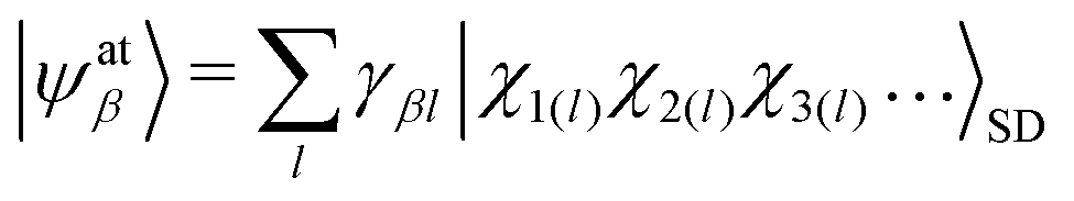
The ERCAR model is a diabatic potential model, which has been developed to account for relativistic couplings, in particular spin–orbit coupling. This approach is extended for the treatment of hyperfine (HF) coupling in the present work. For a proof of principle it is sufficient to account for the HF couplings of the 2S1/2 ground state of hydrogen as well as for the 2P3/2 and 2P1/2 fine structure states of iodine. The basic idea of the ERCAR method is the diabatic representation of the full electronic Hamiltonian in an asymptotic basis where all atoms with strong relativistic effects are separated from the approximately non-relativistic molecular fragment. This separation is key due to the fact, that the relativistic effects are heavily atom centered. This specific diabatic basis representation is utilized in the ERCAR method as given in the following.The full diabatic electronic molecular states |ψdj(Q)〉 can be expanded in the above mentioned direct product basis of the asymptotic states of the relativistic atom |ψatβ(j)〉 with the remaining molecular fragment states |ψfragα(j)(Q)〉. For simplicity, only a single relativistic atom is assumed in the following but the approach is easily expanded to multiple relativistic atoms.45 The jth diabatic state can be written as
| |ψdj(Q)〉 = |ψfragα(j)(Q)〉 ⊗|ψatβ(j)〉, | (1) |
 | (2) |
The full electronic Hamiltonian Ĥel can be separated into a geometry dependent Coulomb Hamiltonian ĤC and a geometry independent Hamiltonian Ĥrel, which describes all the relativistic couplings
| Ĥel(Q) = ĤC(Q) + Ĥrel. | (3) |
| 〈ψdj|Hel(Q)|ψdk〉 = 〈ψdj|HC(Q)|ψdk〉 + 〈ψatβ(j)|Hrel|ψatβ(k)〉 = wdjk(Q) + hreljk | (4) |
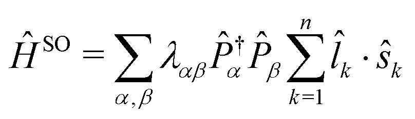
By far the strongest relativistic coupling effect is spin orbit coupling and the ERCAR method was developed primarily to account for SO coupling in diabatic potential models for the quantum dynamics simulation of spectroscopy and reactive scattering processes in excited states. For this purpose, the atomic basis states are expressed in a basis of Slater determinants of spinor orbitals as
 | (5) |
| |χk〉 = |l, ml; s, ms〉. | (6) |
 | (7) |
![[l with combining circumflex]](https://www.rsc.org/images/entities/i_char_006c_0302.gif) k·ŝk act on the kth spinor orbital. The pair of projectors ensures that the couplings are determined for the corresponding atomic states α and β with the corresponding coupling constant λαβ, which in many cases can be obtained from experiment or otherwise is computed by ab initio methods. Especially the use of experimental coupling constants for the atomic states is a great advantage of ERCAR because the ab initio computed SO splittings are way less accurate. E.g., the splitting between the first two fine structure states of the iodine atom, 2P3/2 and 2P1/2, computed ab initio is roughly 10% too small. The representation of ĤSO in the spinor determinant basis eqn (5) yields the final SO coupling matrix to be combined with the diabatic model for the Coulomb Hamiltonian. The treatment of HF coupling follows the same pattern with the appropriate spinor basis and effective operators.
k·ŝk act on the kth spinor orbital. The pair of projectors ensures that the couplings are determined for the corresponding atomic states α and β with the corresponding coupling constant λαβ, which in many cases can be obtained from experiment or otherwise is computed by ab initio methods. Especially the use of experimental coupling constants for the atomic states is a great advantage of ERCAR because the ab initio computed SO splittings are way less accurate. E.g., the splitting between the first two fine structure states of the iodine atom, 2P3/2 and 2P1/2, computed ab initio is roughly 10% too small. The representation of ĤSO in the spinor determinant basis eqn (5) yields the final SO coupling matrix to be combined with the diabatic model for the Coulomb Hamiltonian. The treatment of HF coupling follows the same pattern with the appropriate spinor basis and effective operators.
B. Hyperfine coupling operators
The HF couplings are due to various magnetic and electric interactions between a nucleus and the electronic wave function. The Fermi contact term and the magnetic dipole–dipole interaction are in complete analogy to the magnetic interactions between two electrons represented by the Breit–Pauli Hamiltonian. The only difference is that one electron spin must be replaced by the nuclear spin. The third kind of coupling is the electric quadrupole interaction due to the non-isotropic charge distribution within the nucleus. This interaction of course is not present in the Breit–Pauli Hamiltonian but is easily represented by a corresponding operator. The physical background and derivation of these operators can be found in many textbooks like ref. 52 and 53. We now have a look on each of the three coupling operators.The Fermi contact term has no classical analogon although it often is interpreted as the magnetic interaction between electronic and nuclear magnetic moments of an electron penetrating a finite-sized nucleus. Thus, only electrons in s orbitals contribute to this interaction represented by the operator
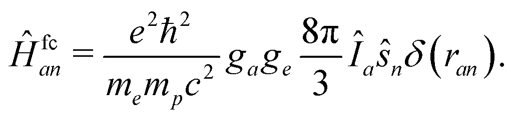 | (8) |
 | (9) |
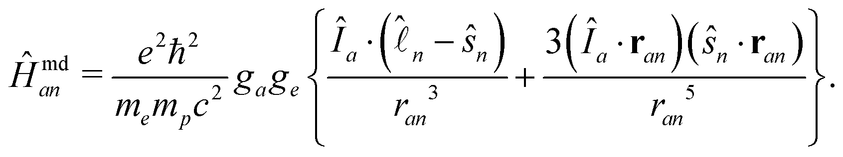
 is the orbital angular momentum operator for electron n and ran is the position vector of electron n with respect to the center of nucleus a. Nuclei with spin greater than 1 also possess an electric quadrupole moment which interacts with the electrons and yields an electric quadrupole term to the full HF interaction Hamiltonian. In general, this can be expressed by
 | (10) |
All these operators in principle could be evaluated numerically by suitable ab initio methods. However, the aim of the ERCAR approach is to yield an analytic diabatic potential model, which requires an analytic evaluation of the couplings for well-defined atomic states. To this end, the operators need to be cast into a form in which they can be evaluated on the basis of spin and angular momentum quantum numbers. The operator Ĥfc is easily represented by a corresponding effective operator because only S states can contribute and the result reads
 | (11) |
![[P with combining circumflex]](https://www.rsc.org/images/entities/i_char_0050_0302.gif) (L=0)an ensures that the nuclear spin and total angular momentum operators act on a specific atomic state with orbital angular momentum L = 0 and with the corresponding coupling constant Afcan. In the present case, such states are only present for the ground state hydrogen atom and thus jH = 1/2. Ĥmd is in complete analogy to the spin–orbit operators and thus can be represented in the same way by an effective operator, yielding
(L=0)an ensures that the nuclear spin and total angular momentum operators act on a specific atomic state with orbital angular momentum L = 0 and with the corresponding coupling constant Afcan. In the present case, such states are only present for the ground state hydrogen atom and thus jH = 1/2. Ĥmd is in complete analogy to the spin–orbit operators and thus can be represented in the same way by an effective operator, yielding | (12) |
(L>0)an ensures that only atomic states with non-vanishing orbital angular momenta contribute. In the present case, only the first two iodine fine structure states with jI = 3/2 and jI = 1/2 are accounted for.
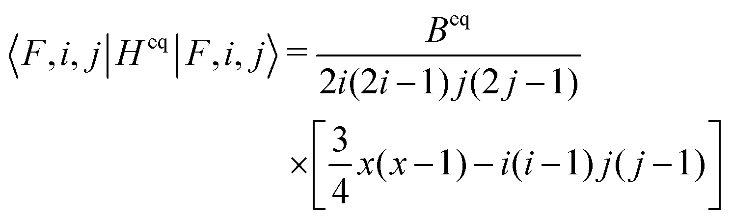
Finally, the operator for the electric quadrupole coupling also needs to be re-cast such that it can be expressed entirely in the Î and Ĵ operators with eigenvalues i and j. This is possible with help of the Wigner–Eckart theorem and yields the effective operator52
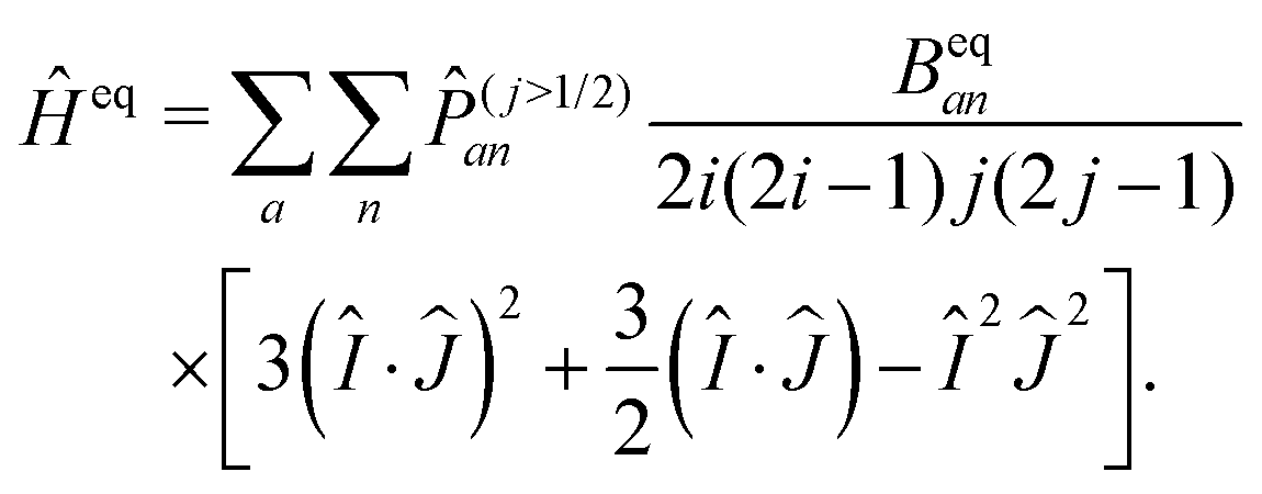 | (13) |
(j>1/2)an ensures that only atomic states with j > 1/2 can contribute, which in the present case is only fulfilled for the iodine ground state with jI = 3/2.
The ERCAR basis states |k, J(k), M(k)J〉 from ref. 44 are fine structure eigenstates with well-defined electronic angular momentum quantum numbers J(k), M(k)J for each asymptotic basis state k. This is important because the HF coupling constants are specific for each atomic fine structure state. However, this basis is insufficient to evaluate the HF coupling operators. Therefore, this basis is transformed first such that the states are eigenstates with respect to the total angular momentum operators ĵ2 and ĵz of each atom and thus can be given as {|k, jI, mIj, jH, mHj〉}. Then, the basis is expanded by the nuclear spinors for each nucleus, which contributes to the HF coupling in a direct product form, thus reading
| |ψk〉 = |k, jI, mIj, jH, mHj〉 ⊗ |iI, mIi〉 ⊗ |iHmHi〉. | (14) |
III. Results
A. Atomic hyperfine coupling matrices
We first treat the H 2S1/2 ground state, which is a particularly simple case. The nuclear spin iH = 1/2 is coupled to the total angular momentum jH = 1/2. The orbital angular momentum is zero and therefore only the contact term needs to be evaluated. The corresponding basis for the H atom can be specified by the four quantum numbers |jH, mHj, iH, mHi〉 and consists of four spinors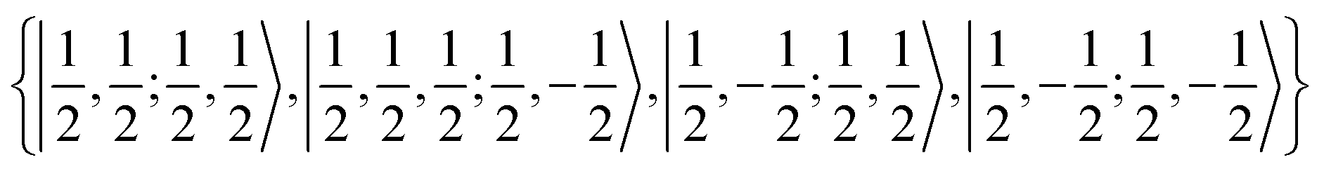 yielding the coupling matrix
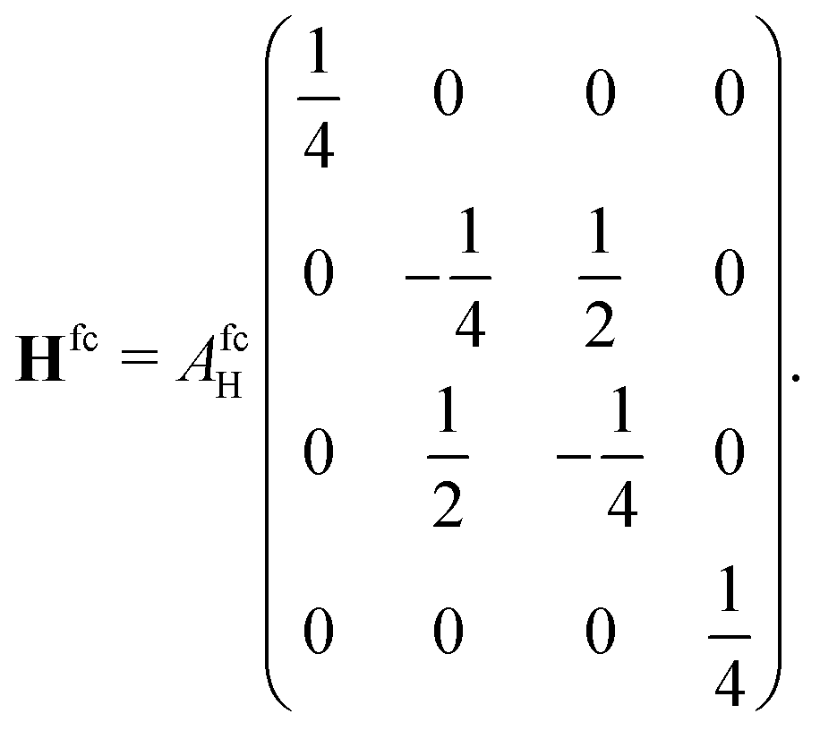 | (15) |
 and one non-degenerate eigenvalue of
  which is the well-known result. Of course, this is also in agreement with the expectation value for the HF eigenstates
 | (16) |
Next, the coupling matrices for the I 2P3/2 fine structure ground state are evaluated. Since the orbital angular momentum of this state is l = 1, the contact term does not contribute but the magnetic dipole–dipole interaction does, which structurally leads to the same coupling matrix. The 127I nucleus has a spin of iI = 5/2 and together with the electronic angular momentum of jI = 3/2 this yields a hyperfine basis of 24 spinors. The representation of the effective magnetic dipole–dipole operator eqn (12) in this spinor basis yields the corresponding coupling matrix, which is given in the supplemental material. The corresponding eigenvalues are 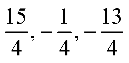 and
and  in agreement with eqn (16) and the corresponding degeneracy numbers.
The spin of iI = 5/2 of the 127I nucleus corresponds to a quadrupole moment, giving rise to electric quadrupole interaction. This interaction is evaluated by use of eqn (13) in terms of the full atomic spinor basis and yields the corresponding coupling matrix given in the supplemental material. Diagonalization of this matrix yields the eigenvalues  and
and  corresponding to values of F = 1, 4, 2, 3. Both eigenvalues and degeneracies are in agreement with the known expectation values given by
 | (17) |
| x = i(i + 1) + j(j + 1) − F(F + 1). | (18) |
 and
and  and the coupling constant from experiment, needed to reproduce the observed spectrum, is AmdI(jI = 1/2) = 219.75 × 10⁻³ cm−1.
B. Hyperfine coupling for H+I
The results from Section IIIA need to be combined with the existing ERCAR model for H+I to yield the HF coupled model for H+I. This is achieved easily by using the full spinor direct product basis eqn (14) and evaluating the corresponding operators eqn (11)–(13). The resulting full HF coupling matrix of dimension 1248 × 1248 is then added to the ERCAR potential model expanded to the same basis. Diagonalization of the fully HF coupled ERCAR model finally yields the HF eigenstates and energies for the full H+I system for any nuclear distance of interest. The results will be analyzed first for the asymptote of the non-interacting atoms. A qualitative level scheme for the lower asymptote corresponding to jI = 3/2 is given in Fig. 1. The splittings are not to scale for clarity. | ||
| Fig. 1 Qualitative level scheme of the asymptotic HF splittings corresponding to H 2S1/2 + I 2P3/2. | ||
The observed pattern can be rationalized by the results for the individual atomic states. First, a splitting into two levels is seen, which corresponds to the well-known HF splitting of the ground state hydrogen atom. Each of the two levels for FH = 0 and FH = 1 are then split up by HF interactions in the iodine atom into four levels corresponding to FI = 1–4. The degeneracy for each of the levels is given by the small numbers in Fig. 1. For scattering calculations, the individual HF eigenstates of the atoms need to be coupled to a new total angular momentum JHF. For instance, the uppermost level in Fig. 1, which results from FH = 1 and FI = 4, yields JHF values of 3, 4, and 5. It is easily seen that the corresponding MHF degeneracies of 7, 9, and 11 add up to the 27 given in Fig. 1. This analysis is quite helpful because as soon as the two atoms start interacting, these degeneracies will be split and the only good electronic quantum number remaining will be ΩHF = |MHF| (ΩSO = |MSO| in case of fine structure states). Note that we label the hyperfine states by the ΩHF quantum numbers in complete analogy to the well-established nomenclature for fine structure states as explained for instance by Herzberg in Chapter VI of ref. 57. Subscripts HF and SO are added to distinguish between hyperfine and fine structure states, respectively. Thus, the above single level with degeneracy 27 will split into 15 levels characterized by ΩHF = 0−, 1, 2, 3, 0+, 1, 2, 3, 4, 0−, 1, 2, 3, 4, 5. All other asymptotic levels will split following an analogous pattern.
The corresponding level splitting situation for the H 2S1/2 + I 2P1/2 asymptote is given in Fig. 2. The qualitative analysis is in complete analogy to the lower asymptote but less levels are observed because FI can only take values of 2 and 3.
 | ||
| Fig. 2 Qualitative level scheme of the asymptotic HF splittings corresponding to H 2S1/2 + I 2P1/2. | ||
C. Distance dependence of the hyperfine eigenstates of H+I
The asymptotic situation is reproduced correctly by the present model, which verifies that the full HF coupling is incorporated correctly into the expanded ERCAR model. This is further confirmed by plotting the HF eigenvalues in comparison with the known fine structure eigenvalues from the original ERCAR model. This plot over the distance range from 2 to 10 a.u. is presented in Fig. 3. | ||
| Fig. 3 Overview of the low-lying fine structure (SO in colour depending on ΩSO) and hyperfine (HF in black) energies for H+I plotted along the inter-atomic distance. | ||
The energies of the lowest 12 fine structure states and 144 HF states along the H–I inter-atomic distance are shown. The HF splittings are not discernible on the scale of that figure because they are five to six orders of magnitude smaller than the fine structure splittings. However, Fig. 3 gives a good overview over the potential curves and demonstrates that the expansion of the ERCAR model to the full 1248 dimensional HF basis was carried out correctly. The two asymptotic fine structure levels due to the I 2P3/2 ground and I 2P1/2 SO excited state are clearly visible. The ground state minimum for the bound HI molecule correlates to the lower asymptote corresponding to a non-degenerate ΩSO = 0+ fine structure state. Similarly, the ΩSO = 0+ fine structure state arising from the SO excited asymptote also forms a shallow minimum and at shorter distance crosses the uppermost ΩSO = 1 fine structure state of the lower state manifold. These general features are not visibly modified by the HF coupling on this scale. Next we will have a closer look at the long-range region of the I 2P1/2 SO excited asymptote.
The energy scale in Fig. 4 is chosen such that the effect of HF coupling on the different fine structure states is visible. On this scale one can see that all fine structure states form shallow minima but the ones corresponding to ΩSO = 0−, 1 are much more shallow with well depths of around 20 to 24 cm−1. The well of the ΩSO = 0+ state is an order of magnitude deeper (760 cm−1) and the H–I distance of the minimum much shorter so that it is not visible in Fig. 4 but can be seen easily in Fig. 3.
 | ||
| Fig. 4 Long-range interaction region of the upper fine structure asymptote H 2S1/2 + I 2P1/2. | ||
Between 11 and 12 a.u. one can distinguish the expected four different hyperfine structure bands. The lowest band aligns with the ΩSO = 0+ fine structure state with decreasing H–I distance while the other three bands are more located around the ΩSO = 0−, 1 fine structure states. Furthermore, the HF splittings corresponding to the ΩSO = 0+, 0− fine structure states depend strongly on the H–I distance and are so small below 9 a.u. that no splittings are discernible anymore on the scale of Fig. 4. However, the splittings can be analyzed numerically. The minimum of the ΩSO = 0− state is located at 7.96109 a.u. and is split into seven hyperfine states with ΩHF = 0+, 1, 0−, 2, 1, 3, 2. The state assignments and splittings between the successive HF states are listed in Table 1. These splittings vary between 14 and 339 MHz, respectively. The ΩHF = 0+, 0− states are distinguished by their eigenvector sign characteristics. The minimum of the ΩSO = 0+ fine structure state is also split into seven hyperfine states with ΩHF = 2, 3, 1, 2, 0+, 1, 0− with significantly smaller splittings between consecutive states compared to the ΩSO = 0− manifold (see Table 1). By contrast, the HF splittings around the minimum of the ΩSO = 1 state are clearly visible in Fig. 4 because the HF splittings are much larger (see Table 1) with an energy difference between the lowest and the highest hyperfine state of around 0.56 cm−1 (16![[thin space (1/6-em)]](https://www.rsc.org/images/entities/char_2009.gif) 745.3 MHz). The HF states around the ΩSO = 1 state are magnified in Fig. 5.
745.3 MHz). The HF states around the ΩSO = 1 state are magnified in Fig. 5.
| Ω SO | 0+ | 0− | 1 | |||
|---|---|---|---|---|---|---|
| r [a.u.] | 5.08680 | 7.96109 | 8.29576 | |||
| Ω HF | ΔE [MHz] | Ω HF | ΔE [MHz] | Ω HF | ΔE [MHz] | |
| 2 | 0+ | 2 | ||||
| 3 | 0.15 | 1 | 35.50 | 1 | 700.26 | |
| 1 | 27.06 | 0− | 61.76 | 1 | 2745.49 | |
| 2 | 0.09 | 2 | 121.18 | 0+ | 662.59 | |
| 0+ | 13.45 | 1 | 21.09 | 0− | 19.24 | |
| 1 | 0.12 | 3 | 338.52 | 0− | 2694.55 | |
| 0− | 0.05 | 2 | 14.38 | 0+ | 203.98 | |
| 1 | 568.54 | |||||
| 1 | 2447.32 | |||||
| 2 | 697.50 | |||||
| 2 | 2351.46 | |||||
| 3 | 701.98 | |||||
| 3 | 2247.73 | |||||
| 4 | 704.66 | |||||
 | ||
| Fig. 5 Further magnification of the long-range interaction region of the ΩSO = 1 state corresponding to the upper fine structure asymptote H 2S1/2 + I 2P1/2. | ||
The HF splittings of the ΩSO = 1 state at 8.29576 a.u. are clearly visible in Fig. 5 and show some regularities. Because the ΩSO = 1 state is degenerate, the state splits into 24 HF components corresponding to 14 distinguishable HF states. In ascending energy order one can assign the HF states with ΩHF = 2, 1, 1, 0+, 0−, 0−, 0+, 1, 1, 2, 2, 3, 3, 4. As can be seen in Fig. 5 the HF states are not split symmetrically around the ΩSO = 1 state. The average energy of the HF states is slightly above the energy of the ΩSO = 1 fine structure state, which is due to couplings to the lower lying fine structure states, in particular those with ΩSO = 0+, 0−. One interesting feature is that most of the splittings can be grouped into two groups, one around 568–700 MHz and one around 2247–2745 MHz (see Table 1). The only exception to these groupings are the small splittings of the four ΩHF = 0+, 0− states which are not degenerate but still follow the regular grouping pattern seen in Fig. 5. Additionally, one pattern is already clearly visible, namely that the HF states always come in sets of seven states with two non-degenerate (ΩHF = 0−, 0+) and five degenerate states. This is easily understood by the nuclear spin multiplicities of 2 × 6 = 12, splitting a given fine structure level into the corresponding HF states. For degenerate fine structure states 24 HF components are observed with 4 non-degenerate and 10 degenerate states. We now will focus on the lower state manifold resulting from the H 2S1/2 + I 2P3/2 asymptote and the corresponding levels are plotted in Fig. 6 for the beginning interaction region on a similar energy scale as above.
 | ||
| Fig. 6 Long-range interaction region of the lower fine structure asymptote corresponding to H 2S1/2 + I 2P3/2. | ||
The hyperfine states shown in Fig. 6, corresponding to the 2P3/2 fine structure states, show similar characteristics as the HF states corresponding to the 2P1/2 fine structure states. Like the ΩSO = 0+ fine structure state in the 2P1/2 manifold, the ΩSO = 0+ fine structure state in the 2P3/2 manifold has a much deeper minimum (−24655 cm−1) (see Fig. 3) at a shorter H–I distance (3.06616 a.u.) than the other 2P3/2 fine structure states. The remaining minima corresponding to this fine structure asymptote are around 14 to 28 cm−1 deep and are located between 7 and 9 a.u. as visible in Fig. 6. The HF states corresponding to the lower ΩSO = 2, 1 states form clearly visible bands around their fine structure states. The order of the HF states characterized by ΩHF as well as the splittings between consecutive states are given in Table 2 for each manifold determined at the minimum distance of the respective fine structure state. The energy difference between the highest and lowest HF state in the ΩSO = 2 band is 6866.41 MHz with the largest splitting between two consecutive states of 872 MHz. The ΩHF = 0+/0− states form two essentially degenerate pairs with a splitting of 183 MHz. The HF states corresponding to the next fine structure state with ΩSO = 1 span an energy range of 6281.11 MHz with maximum splittings between two consecutive states of 881 MHz. This is very similar to the ΩSO = 2 manifold. Again, the ΩHF = 0+/0− states show up in two pairs but show small splittings. The HF states corresponding to the upper fine structure states show significantly smaller splittings and are not discernible on the scale of Fig. 6. The HF states of the ΩSO = 0− manifold are spread over only 443.70 MHz while those corresponding to ΩSO = 1 span a range of 2844.41 MHz. In both cases, the ΩHF = 0+/0− states do not form (quasi) degenerate pairs.
| Ω SO | 0+ | 2 | 1 | 0− | 1 | |||||
|---|---|---|---|---|---|---|---|---|---|---|
| r [a.u.] | 3.06616 | 7.56731 | 8.21910 | 8.60331 | 8.68727 | |||||
| s | Ω HF | ΔE [MHz] | Ω HF | ΔE [MHz] | Ω HF | ΔE [MHz] | Ω HF | ΔE [MHz] | Ω HF | ΔE [MHz] |
| 2 | 1 | 1 | 2 | 2 | ||||||
| 3 | 0.00 | 0− | 706.01 | 2 | 543.27 | 3 | 34.06 | 1 | 512.35 | |
| 1 | 152.44 | 0+ | 0.00 | 0− | 299.46 | 1 | 134.35 | 1 | 317.05 | |
| 2 | 0.00 | 0+ | 182.72 | 0+ | 0.71 | 0− | 58.62 | 0+ | 374.22 | |
| 0+ | 76.22 | 0− | 0.01 | 1 | 479.08 | 2 | 34.07 | 0− | 149.64 | |
| 0− | 0.00 | 1 | 706.01 | 1 | 669.25 | 1 | 137.12 | 0+ | 92.96 | |
| 1 | 0.00 | 1 | 353.38 | 0− | 474.84 | 0+ | 45.48 | 0− | 178.58 | |
| 2 | 706.02 | 0+ | 7.80 | 1 | 248.11 | |||||
| 2 | 524.91 | 2 | 569.94 | 1 | 152.10 | |||||
| 3 | 706.02 | 1 | 541.18 | 2 | 138.36 | |||||
| 3 | 697.59 | 3 | 729.06 | 3 | 140.12 | |||||
| 4 | 706.02 | 2 | 543.62 | 2 | 134.80 | |||||
| 4 | 871.70 | 4 | 881.33 | 3 | 272.53 | |||||
| 5 | 706.02 | 3 | 541.57 | 4 | 133.59 | |||||
Inspection of the overview given in Fig. 3 reveals an interesting feature with potential relevance for H+I scattering or photodissociation. An allowed intersection between the upper ΩSO = 1 fine structure state from the lower asymptotic channel with the low-lying ΩSO = 0+ state from the upper asymptotic channel is observed at a relatively short H–I distance of around 3.8 a.u. This is worth a closer look and a close-up of the region of interest is presented in Fig. 7.
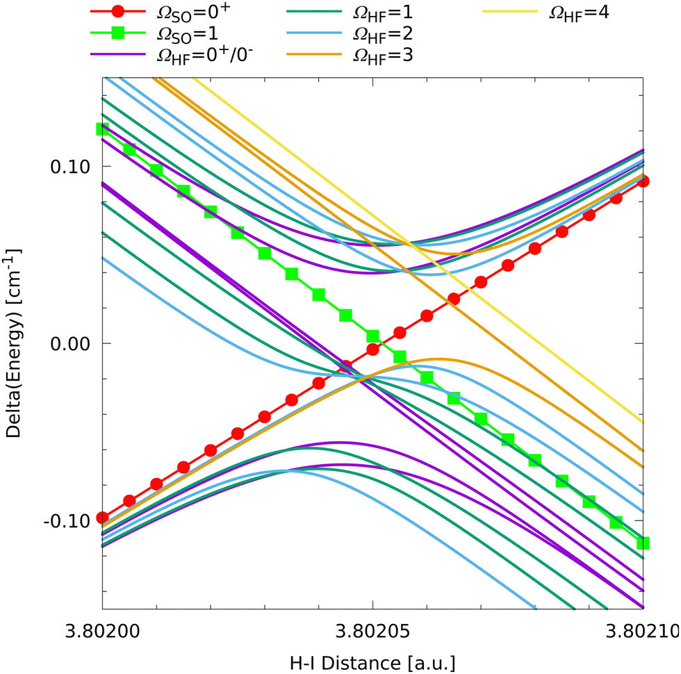 | ||
| Fig. 7 Close-up visualization of the crossing between the ΩSO = 0+ state from the upper and the ΩSO = 1 state from the lower fine structure asymptote at a HI distance around 3.8 a.u. For a better visualization, the average fine structure energy of the two states was subtracted for each distance. | ||
The clearly visible allowed crossing of the fine structure states means that there is no coupling, which is due to symmetry. Thus, in a scattering or reactive process there would be no nonadiabatic population transfer possible between these two states. Only overall rotation could couple these fine structure states but this is a rather slow process compared to a collision or dissociation. The picture changes when looking at the hyperfine states. Except for the ΩHF = 4, the highest ΩHF = 3, and the middle ΩHF = 0+, 0− states, there are couplings between the HF states corresponding to the two different fine structure manifolds. As a result, seven states with ΩHF = 2, 1, 1, 0+, 0−, 2, 3 form weakly avoided crossings, which is the signature of nonadiabatic coupling. Thus, in principle, this could lead to some nonadiabatic population transfer between the fine structure state manifolds even without overall rotation of the system. This will be an interesting feature to study in future scattering and quantum dynamics studies for which the present model has been developed.
We finally turn our attention to the global minimum region and a corresponding close-up is presented in Fig. 8. The fine structure state forming the single global minimum is a non-degenerate ΩSO = 0+ state and conventional chemical wisdom would tell that this is a closed-shell singlet state and not involved in any coupling. However, the HF coupling is leading to the typical set of seven states as was discussed above and a noticeable splitting is observed.
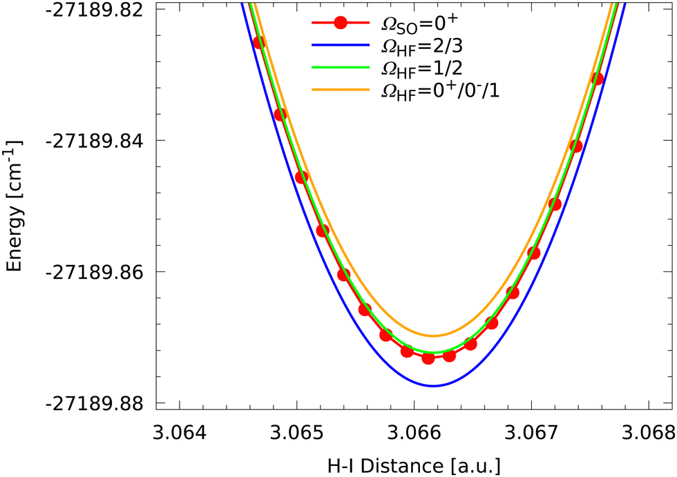 | ||
| Fig. 8 Close-up of the global minimum region of the HI molecule showing the splitting of the hyperfine states due to HF coupling compared to the ΩSO = 0+ fine structure state. | ||
However, inspection of Fig. 8 shows some significant differences to the observations for the higher excited states. First of all, only three different energies are found, which correspond to three groups of degenerate states. The lowest group consists of two states with ΩHF = 2, 3 followed by a degenerate group of two states 152 MHz above with ΩHF = 1, 2. The latter two HF states also seem to be almost coinciding with the ΩSO = 0+ fine structure state. The third degenerate set of states consists of states with ΩHF = 0+, 0−, 1 and is found 76 MHz above. The splittings around the fine structure state are found to be exactly of the ratio 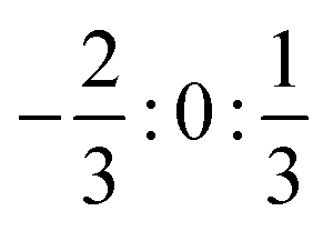 .
.
The HF splitting of the global fine structure ground state might seem counter intuitive at first glance. The usual assumption would be that a simple closed-shell ground state molecule such as HI has a total spin of S = 0 and no unpaired electrons to interact with the nuclear spins. But that of course is a rather simplified and non-relativistic view on the system. A closer and relativistic view of course shows that spin is not a good quantum number anymore and the ground state of HI does not have a total spin exactly but only close to zero. Furthermore, the simplified idea of a “closed-shell” molecule is based on the Hartree–Fock picture of the electronic wave function, meaning that the wave function is a single (closed-shell) Slater determinant. But of course, electron correlation causes the state to be a superposition of many Slater determinants and most of them are open shell and thus would contribute to the relativistic coupling. Spin–orbit coupling leads to a mixing of configuration state functions of different total spin in the ground state wave function causing the computed effect. Although this might seem an unusual observation, it nevertheless is well established and experimentally observable. Brown and Carrington point out in the general introduction chapter of their book on rotational spectroscopy of diatomic molecules that spin–orbit coupling always mixes states of different angular momentum and, thus, generating some orbital (and spin) angular momentum in each state.53 This phenomenon was discussed as early as 1951 by Van Vleck already.58 The ERCAR model accounts for these effects in a straightforward way but using a different basis representation. The diabatic model for the “spin-free” Coulomb Hamiltonian yields for the ground state around the global minimum a mixture of closed-shell ionic atom states (I− + H+) and various open-shell atomic states. This corresponds to the electron correlation and correctly represents the electronic wave functions from ab initio calculations. Adding the fine structure coupling also mixes singlet and triplet basis states as the ERCAR eigenvectors show clearly. The observed non-vanishing splittings of the HF energies of the fine structure ground state are due to the same effect that HF active basis states are contributing to the fine structure state. This means that non-vanishing HF splittings should be present in any molecule that contains nuclei with non-vanishing nuclear spin. In particular, all organic molecules, usually containing many protons, might show this effect to some degree.
While the computed energy splittings cannot be measured experimentally, the effect of HF coupling in closed-shell ground state molecules is well known. The experimental manifestation of this effect is observed in the highly resolved rotational spectra of small molecules. One example of an organic closed shell molecule showing this effect is the argon complex of acetylene, Ar–HCCH.59 HF coupling was measured for the HI molecule as well. The lowest rotational transition in the vibronic ground state of HI shows two distinct hyperfine splittings of roughly 160 and 385 MHz.60–62 These hyperfine splittings are usually explained as nuclear quadrupole couplings with the overall rotation and can be reproduced by appropriate effective Hamiltonians.53 The present ERCAR model does account for the nuclear quadrupole coupling of 127I but also for the magnetic dipole interaction and the Fermi contact interaction with the proton. In contrast to rotational effective Hamiltonians, there are no molecular free parameters in the ERCAR model to be fitted with respect to experimental measurements. The only parameters entering the ERCAR model (besides those of the diabatic Coulomb model) are the atomic coupling constants, which are taken from experimental data, which ensures the highest accuracy possible within the ERCAR framework. In the 2P3/2 ground state of the iodine atom, the hyperfine splittings are dominated by the magnetic dipole rather than the electric quadrupole interaction. The Fermi contact interaction in the hydrogen atom is of a similar order of magnitude. This raises the question why in the simulation of experimental rotational spectra only the quadrupole moment seems to be relevant. This can be investigated using the present model. We studied the effect of the four different coupling constants on the HF splittings of the molecular ground state at the global minimum seen in Fig. 8. It turns out that indeed only the quadrupole coupling contributes significantly to the splittings and the effect of the other coupling constants is absolutely negligible. By contrast, the same analysis yields for all other fine structure states that always magnetic dipole interaction of iodine and Fermi contact interaction of hydrogen contribute heavily to the HF splittings and are not negligible at all. This finding is consistent with the experimental observations53 and gives quite some support that the present ERCAR model represents the physics of the system correctly.
However, the main purpose of the ERCAR model is not to simulate a single experimental feature like a rovibronic transition but much rather to study many excited states and reactive processes or scattering.46 The computed eigenvalues are not an experimental observable and the ERCAR model is not meant to simulate a rotational spectrum. Also note, that ERCAR represents the couplings of the nuclear spins with the electronic wave function rather than the overall molecular rotation. Thus, the observed hyperfine splittings are not directly comparable. Nevertheless, the computed splittings seem compatible with the experimental observations and are in the right order of magnitude. This is quite promising especially in the light of how tiny these energy splittings are.
Another take to assessing the reliability of the new model would be comparison with computed data. The situation is similar to experimental reference data. E.g., hyperfine coupling constants can be computed but are very sensitive to molecular geometry, one-electron basis sets, electron correlation, spin–orbit coupling and so on.63,64 Most usually, they are only computed for the electronic ground state of radicals at the equilibrium geometry. This is the difference to spin–orbit coupling and the corresponding energy splittings, which are directly accessible from electronic structure calculations and also measurable. For SO coupling we showed early on39 by comparison with ab initio computed fine structure energies that the errors introduced by the approximations of the ERCAR method are an order of magnitude smaller than the effect of atomic orbital basis sets or effective core potentials. The ab initio computed SO splitting of the 2P3/2 ground and 2P1/2 SO excited state of the iodine atom is roughly 10% too small while the asymptotic splitting from the ERCAR model is accurate by construction. We assume that the situation for the hyperfine energies will be similar. State-of-the-art computations of HF coupling constants like in ref. 63 also reach an accuracy of roughly ±10% of experimental values while at least the atomic coupling constants of the ERCAR method are accurate because they are the experimentally determined ones. Previous ERCAR results for fine structure energies reach this accuracy not only for the ground but also for excited states without additional computational effort. This means that the method represents the adiabatic electronic states very well in terms of the diabatic asymptotic basis and thus the atomic coupling operators are incorporated with high accuracy into the molecular framework. Whether these atomic coupling operators represent spin–orbit coupling or hyperfine coupling should not make any difference regarding the accuracy of the final results. Finally, we note that ERCAR does not require additional computational effort for the incorporation of HF coupling. The coupling matrix is obtained purely analytically and coupling constants are usually available from experiment. At most the atomic coupling constants would have to be computed if not known for an atomic state of interest. Thus, all computational resources can be used for obtaining the best possible reference data for the Coulomb model. The other important point is that ERCAR by construction yields a fully coupled potential energy model for use in quantum dynamics or scattering studies. Developing such a model based on ab initio fine structure or hyperfine energies seems rather unfeasible for most systems of chemical interest.
IV. Conclusions and outlook
Hyperfine (HF) couplings arising from interactions of nuclear spin with the electronic wave function are of significant interest in many fields and also for technological applications. Theoretical investigations of the quantum dynamics of a molecular system, accounting for the HF interactions properly, requires to incorporate these interactions into the full Hamiltonian of the system. It is of advantage to do this by an analytic model for HF couplings in the sense of a diabatic coupling model, which can be used easily in any general quantum dynamics approach. The Effective Relativistic Coupling by Asymptotic Representation (ERCAR) method was developed exactly for this purpose and yields an analytic diabatic potential energy surface (PES) model including relativistic coupling effects. However, so far it has been applied only to spin–orbit coupling. In this work, the ERCAR approach is extended by the incorporation of HF couplings and a proof of principle study is carried out. The H+I benchmark system is chosen for this purpose since the HF couplings can be added easily to an already existing ERCAR model. The non-vanishing nuclear spins of both atoms, H and I, lead to HF splittings of the fine structure states. The corresponding HF coupling matrices are derived for the 2S1/2 state of H as well as the lowest two fine structure states 2P3/2 and 2P1/2 of I. This is sufficient at least for the present proof of principle study. The relevant HF interactions are the Fermi contact, magnetic dipole–dipole and electric quadrupole term. All these interactions are represented by effective coupling operators, expressed in the form of total nuclear spin Î and total angular momentum Ĵ operators. These operators are represented in the ERCAR basis, which is extended by the nuclear spinors. The explicit expressions for the analytic HF couplings of the 2S1/2 state of H and the 2P3/2 and 2P1/2 states of I are given. The corresponding coupling constants are determined such that the HF model reproduces the experimental atomic hyperfine transitions. The original H+I model containing 104 electronic states is expanded to 1248 states by forming the direct product with the nuclear spinor basis and the HF model is added. Diagonalization of the full ERCAR model yields the HF energy levels and eigenvectors. The asymptotic as well as geometry dependent hyperfine splittings are discussed in detail.Though the overall picture is unchanged with respect to the fine structure states, the HF coupling adds a lot of detail and additional effects to the potential curves. One of these effects is the appearance of additional avoided crossings between the fine structure states, which are due to the HF couplings. First of all, each degenerate fine structure state (ΩSO = 1, 2,…) is split into two distinct sets of hyperfine states. Each of these sets consists of seven hyperfine states, ΩHF = 0+, 0− and five degenerate ones, with a total of 12 state components. This is due to the 12 nuclear spinor basis states corresponding to the spin multiplicities of 2 × 6 for the proton with iH = 1/2 and the 127I nucleus with iI = 5/2. The observed hyperfine splittings within each set are geometry dependent and are particularly large at the asymptote. They are much smaller in the interaction region and range between a few tens to a few thousands of MHz. Quite remarkably, significant splittings of 152 and 76 MHz are observed even at the global minimum of the fine structure ground state. These splittings are almost entirely due to the quadrupole coupling of the 2P3/2 iodine ground state, which is consistent with the interpretation of experimental rotational spectra of closed-shell molecules like HI.
The present HF coupled ERCAR model is sufficient to study the quantum dynamics within the manifold of the lowest two fine structure asymptotes. However, adding the HF interactions for higher asymptotes is straightforward and may improve the accuracy and extend the applicability of the model. We will study the elastic and inelastic scattering dynamics next because this will allow for a direct comparison with our previous study and will reveal the impact of the HF coupling. Since HF couplings and the corresponding splittings should be omnipresent in organic molecules, a future goal will be to develop simple models to account for these effects in more complex molecules.
Data availability
The model developed and presented in the present work is avaliable from the authors upon reasonable request.Conflicts of interest
The authors have no conflicts to disclose.Acknowledgements
The authors are grateful for financial support by the Deutsche Forschungsgemeinschaft (DFG).References
- A. L. Buchachenko, Recent advances in spin chemistry, Pure Appl. Chem., 2000, 72(12), 2243–2258 CrossRef CAS.
- J. R. Woodward, Radical pairs in solution, Prog. React. Kinet. Mech., 2002, 27(3), 165–207 CrossRef CAS.
- C. R. Timmel and K. B. Henbest, A study of spin chemistry in weak magnetic fields, Philos. Trans. R. Soc., A, 2004, 362(1825), 2573–2589 CrossRef CAS PubMed.
- C. T. Rodgers, Magnetic field effects in chemical systems, Pure Appl. Chem., 2009, 81(1), 19–43 CrossRef CAS.
- Y. Morita, S. Suzuki, K. Sato and T. Takui, Synthetic organic spin chemistry for structurally well-defined open-shell graphene fragments, Nat. Chem., 2011, 3(3), 197–204 CrossRef CAS PubMed.
- J. H. Klein, D. Schmidt, U. E. Steiner and C. Lambert, Complete Monitoring of Coherent and Incoherent Spin Flip Domains in the Recombination of Charge-Separated States of Donor-Iridium Complex-Acceptor Triads, J. Am. Chem. Soc., 2015, 137(34), 11011–11021 Search PubMed.
- A. R. Jones, The photochemistry and photobiology of vitamin B12, Photochem. Photobiol. Sci., 2017, 16(6), 820–834 CrossRef CAS PubMed.
- G. Li Manni and A. Alavi, Understanding the Mechanism Stabilizing Intermediate Spin States in Fe(II)–Porphyrin, J. Phys. Chem. A, 2018, 122(22), 4935–4947 CrossRef CAS PubMed.
- T. Ritz, S. Adem and K. Schulten, A model for photoreceptor-based magnetoreception in birds, Biophys. J., 2000, 78(2), 707–718 Search PubMed.
- I. A. Solov'yov, D. E. Chandler and K. Schulten, Magnetic field effects in Arabidopsis thaliana cryptochrome-1, Biophys. J., 2007, 92(8), 2711–2726 CrossRef PubMed.
- J. Cai, G. G. Guerreschi and H. J. Briegel, Quantum Control and Entanglement in a Chemical Compass, Phys. Rev. Lett., 2010, 104(22), 220502 CrossRef PubMed.
- P. J. Hore and H. Mouritsen, The Radical-Pair Mechanism of Magnetoreception, in Ann. Rev. Biophys., ed. K. Dill of Annual Review of Biophysics. Annual Review, 2016, vol. 45, pp. 299–344 Search PubMed.
- H. Zadeh-Haghighi and C. Simon, Magnetic field effects in biology from the perspective of the radical pair mechanism, J. R. Soc., Interface, 2022, 19(193), 20220325 CrossRef CAS PubMed.
- W. A. Coish and J. Baugh, Nuclear spins in nanostructures, Phys. Status Solidi B, 2009, 246(10), 2203–2215 CrossRef CAS.
- W. Wernsdorfer, R. Sessoli and D. Gatteschi, Nuclear-spin-driven resonant tunnelling of magnetisation in Mn12 acetate, Europhys. Lett., 1999, 47(2), 254–259 CrossRef CAS.
- E. M. Pineda, N. F. Chilton, R. Marx, M. Doerfel, D. O. Sells and P. Neugebauer, et al., Direct measurement of dysprosium(III)…dysprosium(III) interactions in a single-molecule magnet, Nat. Commun., 2014, 5, 5243 Search PubMed.
- Y. C. Chen and M. L. Tong, Single-molecule magnets beyond a single lanthanide ion: the art of coupling, Chem. Sci., 2022, 13(30), 8716–8726 RSC.
- I. Zutic, J. Fabian and S. Das Sarma, Spintronics: Fundamentals and applications, Rev. Mod. Phys., 2004, 76(2), 323–410 CrossRef CAS.
- A. R. Rocha, V. M. García-Suárez, S. W. Bailey, C. J. Lambert, J. Ferrer and S. Sanvito, Towards molecular spintronics, Nat. Mater., 2005, 4(4), 335–339 CrossRef CAS PubMed.
- K. Kundu, J. R. K. White, S. A. Moehring, J. M. Yu, J. W. Ziller and F. Furche, et al., A 9.2-GHz clock transition in a Lu(II) molecular spin qubit arising from a 3467-MHz hyperfine interaction, Nat. Chem., 2022, 14(4), 392 CrossRef CAS PubMed.
- P. X. Fu, S. Zhou, Z. Liu, C. H. Wu, Y. H. Fang and Z. R. Wu, et al., Multiprocessing Quantum Computing through Hyperfine Couplings in Endohedral Fullerene Derivatives, Angew. Chem., Int. Ed., 2022, 61(12), e202212939 CAS.
- H. O. H. Churchill, A. J. Bestwick, J. W. Harlow, F. Kuemmeth, D. Marcos and C. H. Stwertka, et al., Electron-nuclear interaction in 13C nanotube double quantum dots, Nat. Phys., 2009, 5(5), 321–326 Search PubMed.
- R. Gehr, J. Volz, G. Dubois, T. Steinmetz, Y. Colombe and B. L. Lev, et al., Cavity-Based Single Atom Preparation and High-Fidelity Hyperfine State Readout, Phys. Rev. Lett., 2010, 104(20), 203602 CrossRef PubMed.
- T. H. Taminiau, J. Cramer, T. van der Sar, V. V. Dobrovitski and R. Hanson, Universal control and error correction in multi-qubit spin registers in diamond, Nat. Nanotechnol., 2014, 9(3), 171–176 CrossRef CAS PubMed.
- E. A. Chekhovich, S. F. C. da Silva and A. Rastelli, Nuclear spin quantum register in an optically active semiconductor quantum dot, Nat. Nanotechnol., 2020, 15, 999–1004 CrossRef CAS PubMed.
- J. Schliemann, A. Khaetskii and D. Loss, Electron spin dynamics in quantum dots and related nanostructures due to hypertine interaction with nuclei, J. Phys.: Condens. Matter, 2003, 15(50), R1809–R1833 CrossRef CAS.
- C. M. Marian, Understanding and Controlling Intersystem Crossing in Molecules, in Ann. Rev. Phys. Chem., ed. M. Johnson and T. Martinez, of Ann. Rev. Phys. Chem. Annual Reviews, 2021, vol. 72, pp. 617–640 Search PubMed.
- T. Ogiwara, Y. Wakikawa and T. Ikoma, Mechanism of Intersystem Crossing of Thermally Activated Delayed Fluorescence Molecules, J. Phys. Chem. A, 2015, 119(14), 3415–3418 CrossRef CAS PubMed.
- S. Kuno, T. Kanamori, Z. Yijing, H. Ohtani and H. Yuasa, Long Persistent Phosphorescence of Crystalline Phenylboronic Acid Derivatives: Photophysics and a Mechanistic Study, ChemPhotoChem, 2017, 1(3), 102–106 CrossRef CAS.
- S. R. May, C. Climent, Z. Tao, S. A. Vinogradov and J. E. Subotnik, Spin-Orbit versus Hyperfine Coupling-Mediated Intersystem Crossing in a Radical Pair, J. Phys. Chem. A, 2023, 127(16), 3591–3597 CrossRef CAS PubMed.
- K. Andres and E. Bucher, Observation of hyperfine-enhanced nuclear magnetic cooling, Phys. Rev. Lett., 1968, 21(17), 1221 CrossRef CAS.
- K. Andres and E. Bucher, Hyperfine Enhanced Nuclear Magnetic Cooling in Van Vleck Paramagnetic Intermetallic Compounds, J. Appl. Phys., 1971, 42(4), 1522–1527 CrossRef CAS.
- K. Andres, Hyperfine enhanced nuclear magnetic cooling, Cryogenics, 1978, 18(8), 473–477 CrossRef CAS.
- D. S. Naik, H. Eneriz-Imaz, M. Carey, T. Freegarde, F. Minardi and B. Battelier, et al., Loading and cooling in an optical trap via hyperfine dark states, Phys. Rev. Res., 2020, 2, 013212 CrossRef CAS.
- H. Liszt, The spin temperature of warm interstellar HI, Astron. Astrophys., 2001, 371(2), 698–707 CrossRef CAS.
- D. A. Neufeld and S. Green, Excitation of interstellar hydrogen-chloride, Astrophys. J., 1994, 432(1, 1), 158–166 CrossRef CAS.
- D. Ben Abdallah, F. Najar, N. Jaidane, F. Dumouchel and F. Lique, Hyperfine excitation of HCN by H2 at low temperature, Mon. Not. R. Astron. Soc., 2012, 419(3), 2441–2447 CrossRef CAS.
- H. Ndome, R. Welsch and W. Eisfeld, A New Method to Generate Spin-Orbit Coupled Potential Energy Surfaces: Effective Relativistic Coupling by Asymptotic Representation, J. Chem. Phys., 2012, 136, 034103 CrossRef PubMed.
- H. Ndome and W. Eisfeld, Spin-Orbit Coupled Potential Energy Surfaces and Properties Using Effective Relativistic Coupling by Asymptotic Representation, J. Chem. Phys., 2012, 137, 064101 CrossRef PubMed.
- N. Wittenbrink, H. Ndome and W. Eisfeld, Toward Spin-Orbit Coupled Diabatic Potential Energy Surfaces for Methyl Iodide Using Effective Relativistic Coupling by Asymptotic Representation, J. Phys. Chem. A, 2013, 117(32), 7408–7420 Search PubMed.
- N. Wittenbrink and W. Eisfeld, An improved spin-orbit coupling model for use within the effective relativistic coupling by asymptotic representation (ERCAR) method, J. Chem. Phys., 2017, 146(14), 144110 CrossRef PubMed.
- N. Wittenbrink and W. Eisfeld, Extension of the Effective Relativistic Coupling by Asymptotic Representation (ERCAR) approach to multi-dimensional potential energy surfaces: 3D model for CH3I, J. Chem. Phys., 2018, 148, 094102 CrossRef.
- N. Weike, E. Chanut, H. Hoppe and W. Eisfeld, Development of a Fully Coupled Diabatic Spin-Orbit Model for the Photodissociation of Phenyl Iodide, J. Chem. Phys., 2022, 156, 224109 CrossRef CAS PubMed.
- N. Weike, A. Viel and W. Eisfeld, Hydrogen–iodine scattering: I. Development of an accurate spin-orbit coupled diabatic potential energy model, J. Chem. Phys., 2023, 159, 244119 CrossRef CAS PubMed.
- N. Weike and W. Eisfeld, The effective relativistic coupling by asymptotic representation approach for molecules with multiple relativistic atoms, J. Chem. Phys., 2024, 160, 064104 CrossRef CAS PubMed.
- N. Weike, W. Eisfeld, K. M. Dunseath and A. Viel, Hydrogen – iodine scattering: II. Rovibronic analysis and collisional dynamic, J. Chem. Phys., 2024, 161, 014302-118 CrossRef PubMed.
- F. Venghaus and W. Eisfeld, Block-diagonalization as tool for the robust diabatization of high-dimensional potential energy surfaces, J. Chem. Phys., 2016, 144, 114110 CrossRef PubMed.
- N. Wittenbrink, F. Venghaus, D. Williams and W. Eisfeld, A new approach for the development of diabatic potential energy surfaces: hybrid block-diagonalization and diabatization by ansatz, J. Chem. Phys., 2016, 145(18), 184108 CrossRef PubMed.
- D. M. G. Williams and W. Eisfeld, Neural network diabatization: a new ansatz for accurate high-dimensional coupled potential energy surfaces, J. Chem. Phys., 2018, 149(20), 204106 Search PubMed.
- D. M. G. Williams and W. Eisfeld, Complete nuclear permutation inversion invariant artificial neural network (CNPI-ANN) diabatization for the accurate treatment of vibronic coupling problems, J. Phys. Chem. A, 2020, 124(37), 7608–7621 Search PubMed.
- N. Weike, F. Fritsch and W. Eisfeld, Compensation States Approach in the Hybrid Diabatization Scheme: Extension to Multidimensional Data and Properties, J. Phys. Chem. A, 2024, 128(21), 4353–4368 CrossRef CAS PubMed.
- M. Weissbluth, Atoms and Molecules, Academic Press, New York, 1978 Search PubMed.
- J. M. Brown and A. Carrington, Rotational Spectroscopy of Diatomic Molecules. Cambridge Molecular Science, Cambridge University Press, 2003 Search PubMed.
- E. Luc-Koenig, C. Morillon and J. Verges, Experimental and theoretical studies in atomic iodine – infrared arc spectrum observations, classification and hyperfine-structure, Phys. Scr., 1975, 12(4), 199–219 CrossRef CAS.
- C. Ashok, S. R. Vishwakarma, H. Bhatt, B. K. Ankush and M. N. Deo, Hyperfine structure measurements of neutral iodine atom (127I) using Fourier Transform Spectrometry, J. Quant. Spectrosc. Radiat. Transfer, 2018, 205, 19–26 Search PubMed.
- C. Ashok, S. R. Vishwakarma, H. Bhatt and M. N. Deo, Hyperfine structure measurements of neutral atomic iodine (127I) in the infrared region (1800–6000 cm−1), J. Quant. Spectrosc. Radiat. Transfer, 2019, 235, 162–179 Search PubMed.
- G. Herzberg, Molecular Spectra and Molecular Structure I. Spectra of Diatomic Molecules, Krieger, Malabar, Florida, 1989 Search PubMed.
- J. H. Van Vleck, The Coupling of Angular Momentum Vectors in Molecules, Rev. Mod. Phys., 1951, 23, 213–227 CrossRef CAS.
- R. L. DeLeon and J. S. Muenter, Structure and properties of the argon-acetylene van der Waals molecule, J. Chem. Phys., 1980, 72(11), 6020–6023 CrossRef CAS.
- M. Cowan and W. Gordy, Further Extension of Microwave Spectroscopy in the Submillimeter Wave Region, Phys. Rev., 1956, 104, 551–552 CrossRef CAS.
- F. C. De Lucia, P. Helminger and W. Gordy, Submillimeter-Wave Spectra and Equilibrium Structures of the Hydrogen Halides, Phys. Rev. A: At., Mol., Opt. Phys., 1971, 3, 1849–1857 CrossRef.
- M. O. Bulanin, A. V. Domanskaya and K. Kerl, High-resolution FTIR measurement of the line parameters in the fundamental band of HI, J. Mol. Spectrosc., 2003, 218(1), 75–79 CrossRef CAS.
- S. Vogler, J. C. B. Dietschreit, L. D. M. Peters and C. Ochsenfeld, Important components for accurate hyperfine coupling constants: electron correlation, dynamic contributions, and solvation effects, Mol. Phys., 2020, 118(19–20, SI), e1772515 CrossRef.
- R. Feng, T. J. Duignan and J. Autschbach, Electron-Nucleus Hyperfine Coupling Calculated from Restricted Active Space Wavefunctions and an Exact Two-Component Hamiltonian, J. Chem. Theory Comput., 2021, 17(1), 255–268 CrossRef CAS PubMed.
Footnote |
| † Electronic supplementary information (ESI) available. See DOI: https://doi.org/10.1039/d4cp04170d |
| This journal is © the Owner Societies 2025 |