Investigation of the effect of solvation on ¹J(Metal–P) spin–spin coupling

Abstract

The solvent effect on the indirect ¹J(M–P) spin–spin coupling constant in phosphine selenoether peri-substituted acenaphthene complexes LMCl₂ is studied at the PP86 level of nonrelativistic and four-component relativistic density functional theory. Depending on the metal, the solvent effect can amount to as much as 50% or more of the total J-value. This explains the previously found disagreement between the ¹J(Hg–P) coupling in LHgCl₂, observed experimentally and calculated without considering solvent effects. To address the solvent effect, we have used polarizable continuum and microsolvated models. The solvent effect can be separated into indirect (structural changes) and direct (changes in the electronic structure). These effects are additive, each brings roughly about 50% of the total effect. For the in-depth analysis, we use a model with a lighter metal, Zn, instead of Hg. A much smaller solvent effect on ¹J(Hg–P) for a dimer form of LHgCl₂ is explained. Pilot calculations of ¹J(M–P) couplings in analogous systems with other metals indicate that for metals preferring square planar structures the solvent effect is insignificant because these structures are fairly rigid. Tetrahedral structures are less constrained and can respond more easily to external effects such as solvation.

---

Introduction

Chelating ligands with soft donor atoms are of great potential interest in coordination chemistry in general, and in homogeneous catalysis in particular. Building on expertise in designing peri-disubstituted naphthalene derivatives that enforce close proximity of heavy chalcogen and pnictogen atoms,¹ we have recently presented a joint experimental and computational study of peri-substituted acenaphthene-based phosphine selenoether ligands derived from Acenap(iPr₂P)(SePh) (L, Scheme 1), and their complexes with selected transition metal centres.² Of particular note was the complex with HgCl₂, which could be characterised through X-ray crystallography both in monomeric and dimeric forms. While density functional.

Scheme 1 Acenap(iPr₂P)(SePh) complexes with metal dichlorides.

computations of the J(Se–P) coupling constants of free L and LHgCl₂ were broadly in agreement with experiment and useful to distinguish between through-space and through-bond nature of these couplings, significant discrepancies were found between experimental and theoretical ¹J(Hg–P) and ¹J(Hg–Se) coupling constants in LHgCl₂ (see Table S3 in the ESI† of ref. 2). In particular, the observed ¹J(Hg–P) coupling, 6610 Hz in CDCl₃, was severely underestimated in calculations at the four-component relativistic BP86 level, which could recover only up to ca. 50% of the observed value. We have now revisited this case computationally, calling special attention to the effect of solvation on the NMR parameters, which was not accounted for in our initial gas-phase calculations. As it turns out, unusually large solvent effects on ¹J(Hg–P) are revealed, which are the subject of the present study.

It should be noted that we do not aim to reproduce experimental values by simulating solvent effects at the best possible level. This would require the use of molecular dynamics simulations with concomitant averaging of four-component relativistic calculations of ¹J(M–P) over a large number of snapshots (as has, for instance, been done previously for ¹J(Pt–Pt) couplings in aqueous solution).³ For systems considered in this work such a procedure would be very time-consuming. Our goal is to investigate the importance of solvent effects on ¹J(M–P) (M = Hg, Zn, Pt, Ni) and to obtain insight into their mechanism. Considering different metals may help us to check whether the importance of solvent effects on ¹J(M–P) depends on the metal.

Computational details

Structures were fully optimised at the PBE0-D3 level of density functional chemistry^4,5 including Grimme's three-body dispersion correction^6–8 using a quasi-relativistic effective core potential along with its (6s5p3d) valence basis on Hg,⁹ Binning and Curtiss’ 962(d) basis on Se,¹⁰ and 6-31G(d) basis elsewhere, together with a fine integration grid (75 radial shells with 302 angular points per shell). Comparable levels have been shown to perform very well for structural parameters of metal complexes from the third transition row.¹¹ The minimum nature of the stationary points has been verified by evaluation of the harmonic vibrational frequencies, which were all real. These computations have been performed using the Gaussian 09 series of programs.¹² The polarizable continuum model (PCM) using the integral equation formalism variant¹³ (IEFPCM) was employed for optimization of structures in solution.^14–16

Relativistic calculations of indirect spin–spin coupling constants (sscc) have been performed utilizing the four-component methodology based on the Dirac–Coulomb Hamiltonian as implemented in the ReSpect program.^17–19 To estimate solvent effects in the relativistic sscc calculations we have employed the IEFPCM methodology as described in ref. 20 employing two different parametrisations described in ref. 21 and 22 denoted as PCM-1 and PCM-2, correspondingly (which differ in the choice of radii for the interlocking atomic spheres from which the cavity is constructed, see Table S1 in the ESI†). In the relativistic sscc calculations the PCM contribution to response Dirac–Kohn–Sham equations vanishes and it appears only in the perturbation-free SCF as described in ref. 20. This is because in the closed-shell (Kramers-restricted) case while utilizing DFT functionals without exact-exchange contribution, the response electron charge density and the terms involving the restricted magnetically balanced basis for the small component of the four-component wavefunction vanish. See also ref. 17 where a similar case of Coulomb contribution to the Fock matrix is discussed. Dyall's uncontracted valence double-zeta basis^23,24 was used for Hg, Zn, Pt and Ni. Dyall's uncontracted valence double-zeta basis augmented with diffuse functions²⁵ was employed for Se and uncontracted IGLO-II²⁶ on H, C, P, and Cl. For easier comparison of data for different metals, we also included reduced coupling constants K(M–P) in some tables.

Analysis of ¹J(Zn–P) was done at the non-relativistic level. The non-relativistic calculations were done with a local modified version of the deMon-KS code.^27,28 In both relativistic and non-relativistic calculations, we employed the PP86 exchange–correlation functional in its spin-unrestricted formalism.²⁹ IGLO-II basis set was used for all atoms except Zn, for which we use a slightly modified TZV basis from ref. 30. The basis set used for Zn is shown in the ESI.† For localization of orbitals, we used the Pipek–Mezey³¹ and Boys³² procedures. In the non-relativistic calculations, we have analysed only the Fermi-contact contribution that was by far dominating (see Table S2, ESI†). The DrawMol program³³ was used for visualization of coupling deformation density³⁴ and localised molecular orbitals.

Results and discussion

The Hg complex LHgCl₂ was special in that it could be crystallised as monomer or as dimer, depending on the solvent (CH₂Cl₂vs. CHCl₃, respectively). A previously calculated value of ¹J(Hg–P) for monomeric LHgCl₂ obtained without consideration of solvent effects significantly deviates from the experimental value (obtained in CDCl₃), whereas the calculated result for the dimer is in better agreement with experiment. Fig. 1 shows the gas-phase optimized structures and the corresponding J-values.

Fig. 1 Hg complex LHgCl₂ (left) and its dimer (right). Relativistic gas-phase calculations of ¹J(Hg–P) were done for gas-phase optimized structures.

Based on this finding it might be tempting to speculate that it is the dimer, rather than the monomer that is present in this solution, in accord with the structures in the solid state. However, for other derivatives, e.g. with a bulkier mesityl instead of a phenyl group on Se, no evidence for occurrence of a dimer was obtained, and very similar ¹J(Hg–P) couplings around ca. 6100–6200 Hz were obtained by NMR in the liquid and in the solid-state (where in the latter the structure is monomeric).

In our initial gas-phase calculations on monomeric LHgCl₂, we already found a notable dependence of the computed coupling on structural parameters, in particular the Cl–Hg–Cl bond angle. This angle differed noticeably between the gas-phase optimised structure and that observed in the solid state, suggesting that there could be a large sensitivity of structural and, hence spectroscopic parameters on the surrounding medium. To probe to what extent this could also be the case for the monomer in solution, we decided to investigate solvation effects for this species in more detail.

Direct and indirect solvent effects

The presence of solvent can affect a calculated property in two ways: by changing the geometrical parameters of the structure (indirect effect) and by changing the electronic structure (direct effect). In order to estimate the indirect solvent effect on ¹J(Hg–P) for the Hg monomer we performed a series of gas-phase calculations for geometries obtained from different sources (see Table 1). We considered a gas-phase optimized structure (the second column), the experimental X-Ray structure with relaxed positions of protons (the third column) and structures with two explicitly present solvent molecules optimized with and without inclusion of bulk solvent effects via polarised continuum model (PCM, fifth and fourth columns, respectively). The last two structures are very crude models for the situation in solution but they can give us a first glance on the indirect solvent effect. The presence of two solvent molecules increases the ¹J(Hg–P) value by about 50%. Comparing the structures used for Table 1 we found that they differ mainly in the Cl–Hg–Cl angle (see the second row), which ranges from 102.2 deg for the X-ray structure to 122.2 deg for the gas-phase optimized structure. The angles for the structures with two solvent molecules are somewhere in the middle (113.1 deg and 106.4 deg). Note that according to the data in Table 1, the smaller the Cl–Hg–Cl angle the bigger ¹J(Hg–P). Before investigating the dependence of ¹J(Hg–P) on the Cl–Hg–Cl angle in more detail (see Fig. 2), let us get a first estimation of the direct solvent effect (see Table 2).

Table 1 Gas-phase calculated ¹J(Hg–P) for differently optimised structures of LHgCl₂, the resulting Cl–Hg–Cl angle and the Hg–P distance. ¹K(Hg–P)/Hz are given in parentheses

Geometry	Optimised (gas-phase)	X-Ray (H relaxed)	Optimised with 2 CHCl3 (gas-phase)	Optimised with 2 CHCl3 (PCM-1)	Exp.
^1J(Hg–P)/Hz	2041.5 (891.5)	3485.5 (1522.2)	2949.8 (1288.2)	3087.9 (1348.5)	6610.7 (2887)
^1K(Hg–P)/Hz
Cl–Hg–Cl/deg.	122.8	102.2	113.1	106.4
R(Hg–P)/Å.	2.53	2.41	2.48	2.50

---

Fig. 2 Dependence of the total energy of monomeric LHgCl₂ on the Cl–Hg–Cl angle.

Table 2 ¹J(Hg–P) in LHgCl₂ calculated with PCM, ¹K(Hg–P)/Hz are given in parentheses

Geometry	Optimised (PCM; CHCl3)	Optimised (PCM; CH2Cl2)	Optimised with 2CHCl3 (PCM; CHCl3)	Exp.
^1J(Hg–P)/Hz, PCM-1	4193.1 (1831.2)	4478.4 (1955.8)	3987.9 (1741.6)	6610 (2887)
^1J(Hg–P)/Hz, PCM-2	5108.2 (2230.8)	5670.4 (2476.3)
Cl–Hg–Cl/deg.	104.4	101.7	106.4
R(Hg–P)/Å.	2.47	2.48	2.50

---

For Table 2 we used the structures optimized with different options for inclusion of solvent effects: PCM simulating chloroform (second column) and dichlormethane (third column) and also the PCM optimized structure with two solvent molecules (fourth column). The direct solvent effect on J-couplings simulated by PCM is huge and greatly depends on technical details of the PCM setup (compare the values in the second column obtained with PCM-1 and PCM-2 options, which differ in the choice of the radii of the interlocking spheres around the atoms, from which the molecular cavity is constructed, see Table S1 in the ESI†). This finding reminds us that the use of PCM models is expected provide only a qualitative description of solvent effects. The data in Tables 1 and 2 show that the direct and indirect solvent effects work in accord, both increasing the value of ¹J(Hg–P). Their relative magnitude is comparable. The gas-phase calculations of ¹J(Hg–P) give J-values from about 2050 to 3500 Hz depending on the Cl–Hg–Cl angle (Table 1), whereas the PCM values range from about 4000 to 5700 Hz.

The dependence of ¹J(Hg–P) on the Cl–Hg–Cl angle seen in Table 1 calls for further investigation. For this we considered a series of structures with the different fixed value of the Cl–Hg–Cl angle and all other geometrical parameters reoptimized. The Cl–Hg–Cl angle was varied from 95 to 125 deg. with a step of 5.0 deg. Note that the variation of the Cl–Hg–Cl angle in the range of 30 deg. caused only less than 4 kcal mol⁻¹ changes in the total energy (see Fig. 2). This means that the angle between the two Hg–Cl bonds can easily change due to solvent effects (or packing effects in a crystal). The plot in Fig. 3 confirms a strong monotonous dependence of ¹J(Hg–P) on the Cl–Hg–Cl angle. The largest J-value of about 3400 Hz was obtained for the Cl–Hg–Cl angle of 95 deg and the smallest of about 1880 Hz corresponds to the angle of 125 deg (gas-phase calculations). The inclusion of solvent effects for the geometry optimization with a fixed value of the Cl–Hg–Cl angle has minor effect on the calculated J-values (compare the yellow and blue lines in Fig. 3). This means that the Cl–Hg–Cl angle is the most important structural parameter influenced by solvent effects. Due to the electrostatic attraction between the partial negative charge of the chlorine atoms and the protic sites of the mildly polar solvent molecules the Hg–Cl bonds become longer and the centers of charge of the Hg–Cl bonds slightly shift away from Hg, which in turn serves to reduce the Cl–Hg–Cl angle.

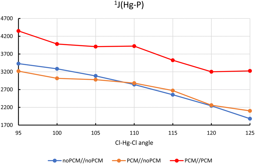Fig. 3 Dependence of ¹J(Hg–P)/Hz on the Cl–Hg–Cl angle in LHgCl₂. A//B denotes the use of PCM (geometry optimization//calculation of J).

Inclusion of PCM for the calculation of ¹J(Hg–P) shifts the J-values up further by about 1100 Hz (red line in Fig. 3), confirming our previous observation that indirect and direct solvent effects are additive.

PP86 gas-phase calculations

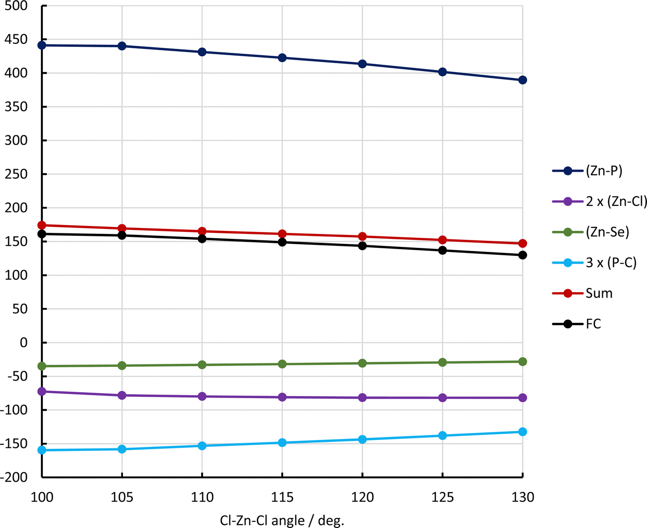
Four-component relativistic calculation of J-couplings is a relatively new area of quantum chemistry, and not all the tools for analysing the computed J-couplings have been implemented yet that are available at the non-relativistic level. Moreover, the adoption of these tools is hindered by the complex nature of multicomponent wavefunctions in the relativistic framework, which is further complicated by the fact that the familiar concepts and terminology used by chemists are based on non-relativistic or scalar-relativistic molecular orbitals. Therefore, to be able to conduct more in-depth analysis, we consider also a model with a lighter metal, Zn, instead of Hg. Dependence of ¹J(Zn–P) on the Cl–Zn–Cl angle in LZnCl₂ is presented in Fig. 4. Again, for each structure all other than the Cl–Zn–Cl angle geometrical parameters were reoptimized.

Fig. 4 Dependence of ¹J(Zn–P)/Hz on the Cl–Zn–Cl angle in LZnCl₂. noPCM//noPCM calculations.

The similarity of graphs in Fig. 3 and 4 justifies the consideration of the model with Zn for further analysis. The much smaller quantitative effect on J for Zn compared to Hg, is in part due to the smaller gyromagnetic ratio of the former, but also apparent in the reduced coupling constants, K, which are much higher (by a factor of 5 or so) for Hg than for Zn, compare values in parentheses in Table 2. The smaller K-values for Zn compared to Hg are likely caused by scalar relativistic effects which are much stronger for Hg.

The dependence of the ¹J(M–P) couplings on the Cl–M–Cl angle can be partially explained by the corresponding changes in other structural parameters (see Table 3). For smaller Cl–M–Cl angles due to increased electrostatic repulsion the M–Cl bonds become longer.

Table 3 R(M–Cl), R(M–P), R(M–Se) (in Å), M = Hg, Zn for the scans of Cl–M–Cl angle in LMCl₂

< Cl–M–Cl/deg.	95	100	105	110	115	120	125	130
a Mean R(M–Cl) value.
M = Hg
R(Hg–Cl)^a		2.46	2.46	2.46	2.45	2.45	2.45	2.44
R(Hg–P)		2.44	2.45	2.47	2.48	2.50	2.51	2.54
R(Hg–Se)		2.87	2.87	2.87	2.87	2.87	2.88	2.88
M = Zn
R(Zn–Cl)^a	2.23	2.23	2.22	2.22	2.22	2.21	2.21
R(Zn–P)	2.35	2.34	2.35	2.36	2.36	2.37	2.38
R(Zn–Se)	2.55	2.54	2.55	2.55	2.56	2.57	2.57

---

In turn, the M–P bond becomes shorter (by 0.1 Å. for Hg and 0.03 Å. for Zn in the range of 30 deg). This contributes to bigger J-values for smaller angles (see also Fig. 5). Interestingly, the length of M–Se bond is much less affected by the Cl–Hg–Cl angle. Note, that these trends are similar for Hg and Zn.

Fig. 5 Dependence of LMO contributions to ¹J(Zn–P)/Hz on the Cl–Zn–Cl angle in LZnCl₂. Pipek–Mezey localization.

Looking at the contributions from individual localized orbitals to ¹J(Zn–P) as a function of the Cl–Zn–Cl angle (Fig. 5), it appears that the largest contribution to ¹J(Zn–P) comes from the (Zn–P) bond, which is expected for this one-bond coupling. Contributions from other bonds involving either Zn or P are negative. The strongest dependence on the Cl–Zn–Cl angle is exhibited by the contribution from the (Zn–P) bond (compare with the dependence of R(Zn–P) on the angle). This effect is somewhat diminished by the negative contribution from the three Sigma (P–C) bonds (yellow line). Surprisingly, the contribution from the (Zn–Cl) bonds practically does not depend on the Cl–Zn–Cl angle.

Microsolvated models

PCMs only account for bulk solvation effects in an approximate way. To account for possible specific solvent–solute interactions that are not accounted for in these models microsolvated clusters with explicit CHCl₃ molecules have been optimized (starting from structures with the CH bond of the latter pointing toward the Cl ligands, see Fig. 6 for the optimised structures).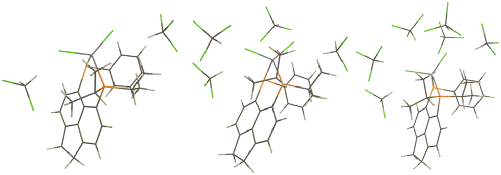

Fig. 6 Microsolvated Zn models; LZnCl₂ + 2CHCl₃ (left), LZnCl₂ + 4CHCl₃ (middle), and ZnLCl₂ + 6CHCl₃ (right).

Interestingly the PCM//PCM result is well reproduced with 6 solvent molecules (see Table 4). ¹J(Zn–Se) and ¹J(P–Se) are almost not affected by solvent effect. Apparently, P and Se are much better shielded from the environment compared to the Cl atoms, which protrude into the solution and, due to their rather high negative charge density (see plot of electrostatic potential in Fig. 7) can engage in electrostatic interaction even with a mildly polar solvent. This may rationalise why ¹J(P–Se) is not much affected by solvation. No simple explanation can be seen why ¹J(Zn–Se) is so insensitive to the Cl–Zn–Cl angle, when ¹J(Zn–P) is very sensitive.

Table 4 ¹J(Zn–P)/Hz calculated for microsolvated models, ¹K(Zn–P)/Hz are given in parentheses. Four-component relativistic calculations

	^1J(Zn–P)	^1J(Zn–Se)	^1J(P–Se)
no-PCM//no-PCM	136.7 (172.5)	−60.2 (−160.7)	13.2 (5.5)
PCM//PCM-1	178.6 (225.4)	−56.7 (−151.4)	16.8 (6.9)
+2CHCl3; no-PCM//no-PCM	156.0 (196.9)	−60.2 (−160.7)	11.9 (4.9)
+2CHCl3; no-PCM//PCM-1	180.3 (227.6)	−56.4 (−150.6)	13.4 (5.5)
+4CHCl3; no-PCM//no-PCM	167.8 (211.8)	−59.2 (−158.0)	14.2 (5.9)
+6CHCl3; no-PCM//no-PCM	187.5 (236.7)	−42.5 (−113.4)	14.4 (6.0)

---

Based on our experience with microsolvated models for Zn, we considered a microsolvated model with 6CHCl₃ molecules for LHgCl₂ (see Fig. 8). For this model, the calculated values of ¹J(Hg–P) are 3846.9 Hz (no PCM) and 4210.2 Hz (PCM-1). The value of the Cl–Hg–Cl angle is about 103.4 deg. Similarly to Zn, the inclusion of six solvent molecules allows one to practically replicate the PCM result. It is remarkable that simple optimisation in the continuum brings about a similar structural change as found in the microsolvated structures (see Table 2).

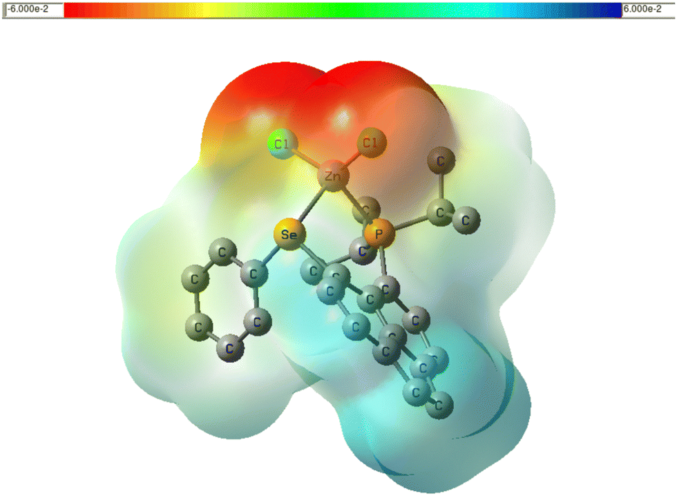Fig. 7 Plot of electrostatic potential of LZnCl₂ in the gas phase, color-coded from 0.06 a.u. (red) to +0.06 a.u. (blue) and mapped onto an isodensity surface (ρ = 4 × 10⁻⁴ a.u.), PBE0 level.

Fig. 8 A microsolvated LHgCl₂ model with 6 solvent molecules.

Coupling deformation density³⁴ (CDD) is the difference between the electron densities of a system when the nuclear moments of the interacting nuclei are parallel and antiparallel. CDD shows which parts of the electron density are involved in transmission of the interaction of nuclear magnetic moments. We calculated CDD for ¹J(Zn–P) for the model with six solvent molecules and the model without solvent molecules but with the same structure. Plotting the difference between these two CDDs allows us to visualize the direct solvent effect on ¹J(Zn–P). Fig. 9 shows that the electron density of solvent molecules does not directly contribute to CDD. This explains the similarity of the results obtained with PCM and for the microsolvated model. The solvent affects CDD mainly in the area close to chlorine atoms and along the Zn–P bond.

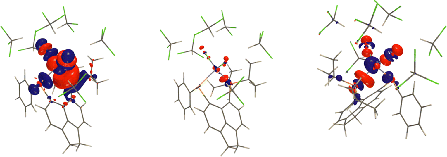Fig. 9 The total CDD for ¹J(Zn–P) for the model with 6 CHCl₃ with isosurface value of 0.04 a.u. is shown on the left. The middle and right plots show the solvent effect on the CDD obtained as the difference between the CDD for the microsolvated model and the model without solvent molecules but the same structure. The middle plot was obtained with isosurface value of 0.04 a.u. and the right one with 0.2 a.u.

Non-relativistic calculations allowed us to decompose the total ¹J(Zn–P) value into contributions from individual molecular orbitals, either canonical or localised. We collected the most important LMO contributions to ¹J(Zn–P) in Table 5. The difference between the corresponding numbers in the last two rows shows the contribution from the LMOs not included in Table 5. The data in the first column are obtained without consideration of solvent effects. The third column presents the results for the model with six solvent molecules and the data in the second column are obtained for the same structure but without solvent molecules. The differences between the data in second and third columns show the indirect solvent effect on individual LMO contributions. Comparison of the numbers in the last two columns allows one to address the direct solvent effect.

Table 5 LMO contributions (in Hz) to ¹J(Zn–P) in LZnCl₂

LMO^a	ZnLCl2^b	ZnLCl2, frozen^c	ZnLCl2 + 6CHCl3
a Pipek–Mezey localization. b Gas-phase structure. c “Frozen” means the same structure as the structure of the microsolvated model (third column) but without solvent molecules.
Zn–P	393.5	450.1	477.0
2 × (Zn–Cl)	−82.1	−82.6	−64.7
Zn–Se	−28.3	−33.7	−35.7
3 × (P–C)	−134.6	−160.0	−184.1
Sum	148.6	171.2	192.5
FC	132.0	154.4	178.3

---

The contribution of the Zn–P bond is more affected by structural changes due to solvent (increase by 56.6 Hz) than by the changes in the electronic structure (26.9 Hz). The overall solvent effect on the contribution of the Zn–P bond (83.5 Hz) is diminished by the negative contribution from the P–C bonds (−49.5 Hz). Interestingly, the contributions of the Zn−Cl bonds are more affected by the changes in the electronic structure than by the changes in the geometry due to solvent effects. In the “frozen” structure the centre of charge of the LMO representing the Zn–Cl bond is only slightly closer to Cl than in the gas-phase structure (0.55 A and 0.56 A, correspondingly). In the microsolvated structure this distance is 0.51 A. We also performed the LMO analysis of ¹J(Zn–P) using Boys localization. These data are presented in Table S3 (ESI†). Both localizations gave qualitatively consistent pictures.

Since the main effect comes from the Zn–P bond, it is logical to concentrate on the analysis of its contribution to ¹J(Zn–P). With Pipek–Mezey localization, its bond order is increasing upon solvation from 0.227 (gas-phase structure) to 0.234 for the micro-solvated model. The bond order of Boys localized LMO remains practically unchanged (0.270 and 0.271). In the presence of the Fermi-contact interaction, the Zn–P bond becomes spin-polarised due to an admixture of originally vacant orbitals of the system without magnetic interactions. For deeper analysis we can look at the contributions from individual vacant orbitals admixed to σ(Zn–P), in other words from individual excitations from this orbital. In order to efficiently contribute to spin-polarisation of a particular occupied orbital, an admixed vacant orbital must be overlapping with the occupied orbital (see discussion in ref. 35 and 36). Therefore, it is not surprising that by far the biggest contributions come from excitations to antibonding Zn–P and Zn–Cl orbitals. These contributions are presented in Table 6. The computational procedure used for obtaining these contributions is described in ref. 36 and briefly recapitulated in the ESI.† The overlap of densities of LMOs representing σ. (Zn–P) and σ*(Zn–Cl) is shown in Table S4, ESI.†

Table 6 The most important excitations due to the Fermi contact interaction from σ(Zn–P) to vacant LMOs: Contributions to ¹J(Zn–P) in Hz

	ZnLCl2^a	ZnLCl2, frozen^b	ZnLCl2 + 6CHCl3
a Gas-phase structure. b “Frozen” means the same structure as the structure of the microsolvated model (third column) but without solvent molecules. c In case of the microsolvated structure the localized σ*(Zn–Cl) orbitals were presented separately and in case of the gas phase structure the localization procedure produced a symmetric linear combination of these orbitals.
σ*(Zn–P)	252.9	256.6	257.7
σ*(Zn–Cl) × 2^c	110.8	140.3	179.1
Sum	363.7	396.9	436.8

---

The difference between the values in the last row in Table 6 show the indirect solvent effect due to the considered excitations (396.9–363.7 = 33.2 Hz) and the direct solvent effect (436.8–396.9 = 39.9 Hz). These data indicate that most important changes due to solvent is experienced by the antibonding Zn–Cl orbitals. Plots of considered vacant LMOs are shown in the ESI.† A smaller Cl–Zn–Cl angle increases the overlap of the densities of σ(Zn–P) and antibonding Zn–Cl orbitals and the interaction with the solvent enhances the effect (see Table S4, ESI†). It should be noted that the total solvent effect is an interplay of contributions from different excitations (see Fig. S2, ESI†). Here we have considered only the most important ones.

We assume that the same qualitative arguments will apply to the contributions to the J-couplings in the Hg congeners. We note that quantitatively K is much larger for Hg than for Zn. Arguably, this is related to factors such as increased scalar relativistic effects on the hyperfine structure,³⁷ a softer, more polarizable d shell, and smaller separations between occupied and virtual MOs (leading to smaller energy denominators in perturbation expressions), on going from Zn to Hg, but this should not affect the more qualitative aspects of our analysis.

One may expect that the structural flexibility with respect to the Cl–M–Cl angle is particularly pronounced for tetrahedral d¹⁰ metal complexes. To confirm this, we also optimized two analogous d⁸ complexes (M = Ni, Pt), which adopt a square planar structure with a more rigid bond angle close to 90 deg. As expected, little variation of this angle is found upon solvation (just modelled with PCM) and, thus, only a relatively small solvent effect is predicted (Table 7).

Table 7 The solvent effect on ¹J(M–P)/Hz and ¹J(M–Se)/Hz in LMCl₂, M = Ni, Pt. The corresponding K-values/Hz are given in parentheses

	^1J(Ni–P)	^1J(Ni–Se)	Cl–Ni–Cl angle	^1J(Pt–P)	^1J(Pt–Se)	Cl–Pt–Cl angle
noPCM//noPCM	−207.3 (234.6)	7.5 (−4.0)	97.46	3072.5 (8476.8)	−552.4 (−720.6)	97.11
PCM//PCM-1	−212.2 (240.1)	−0.4 (0.2)	96.41	3184.8 (8786.6)	−508.3 (−663.1)	95.82

---

So far, we have concentrated on the solvent effect on J-couplings in monomeric LMCl₂ complexes. We can now also revisit the dimer for M = Hg (see Fig. 1). The computed ¹J(Hg–P) value changes from 5418.8 Hz in the gas phase to 5792.3 Hz and 6091.8 Hz with PCMs using the parameters of CHCl₃ and CH₂Cl₂, respectively (PCM was employed for both structure optimisation and J-coupling calculation; the Hg–P bond lengths and the Cl–Hg–Cl angles in the three structures are given in Table S5 in the ESI†). Even though this computed increase in ¹J(Hg–P) would seem to improve the agreement with experiment (6610.7 Hz in CD Cl₃,), overall there is a much smaller solvent effect on this property for the dimer than for the monomer. Given the large sensitivity of the results on the particular PCM model (see Table 2), unfortunately it is not possible at this stage to unambiguously assign the aggregation state in solution based on the computed J couplings.

Why is the solvent effect for the Hg dimer less important for the dimer than for the monomer? We have shown that the interactions of the chlorine atoms with the solvent are responsible for the solvent effect on ¹J(M–P) in these complexes. In the dimer, one of the chlorines is shielded from the solvent by another unit, greatly diminishing the solvent effect. This can be seen in the plots of electrostatic potentials for Hg monomer and dimer shown in Fig. 10. Also, the Cl–Hg–Cl angle in the dimer is significantly smaller than in the monomer even for the gas-phase structures (see Table S5 in the ESI†).

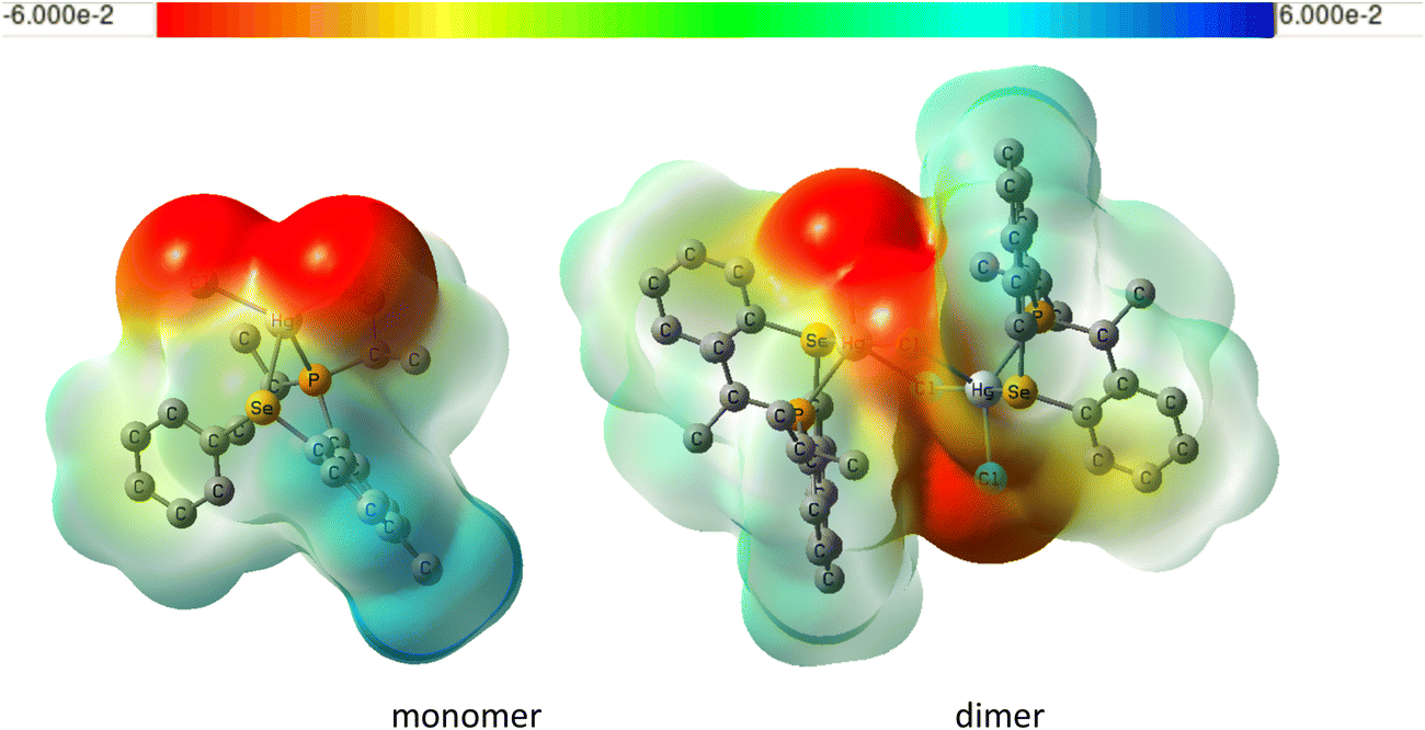Fig. 10 Plot of electrostatic potential of monomeric and dimeric LHgCl₂ (same level and settings as in Fig. 7).

Conclusions

In this article we investigated the solvent effect on ¹J(M–P) in phosphine selenoether peri-substituted acenaphthene complexes LMCl₂. Depending on the metal, the solvent effect can amount to as much as 50% or more of the total J-value. This explains the previously found disagreement between the ¹J(Hg–P) coupling in LHgCl₂, observed experimentally and calculated without considering solvent effects.

The solvent effect can be separated into indirect (structural changes) and direct (changes in the electronic structure). These effects are additive, each brings roughly about 50% of the total effect. The main indirect effect is the decrease of the Cl–M–Cl angle which can be explained on electrostatic grounds: due to the presence of the solvent, the centres of charge of the M–Cl bonds move toward Cl resulting in a smaller Cl–M–Cl angle. For ZnLCl₂, the mean distance between the centre of charge and chlorine atoms is 0.56 Å and 0.51 Å for the gas-phase and microsolvated structures, correspondingly. The M–Cl bonds become longer and the M–P bond becomes shorter. Consequently, the value of ¹J(M–P) increases. The length of the M–Se bond is not affected as much and ¹J(M–Se) almost does not depend on the Cl–M–Cl angle.

To address the direct solvent effect, we have used PCM and microsolvated models. In order to reproduce the PCM results it has been necessary to explicitly include six solvent molecules. A smaller number of solvent molecules is found insufficient. Analysis of contributions from localized molecular orbitals reveals that the strongest contributions to the solvent effect is due to excitations from σ(Zn–P) to σ*(Zn–Cl) orbitals. This can be rationalized as follows. The main contribution to one bond couplings comes from the bond connecting the two coupled nuclei. In general, vacant MOs are more delocalized than occupied ones and therefore they may be more affected by the electrostatic potential of the solvent. Amongst vacant LMOs, the closest to the solvent are σ*(Zn–Cl) orbitals. Moreover, the presence of easily polarisable lone pairs of chlorines increases the effect. A much smaller solvent effect on ¹J(Hg–P) for the Hg dimer can be explained the fact that one of the chlorines is shielded from solvent by another unit. Also, the Cl–Hg–Cl angle in the dimer is significantly smaller than in the monomer even for the gas-phase structures.

Pilot calculations of ¹J(M–P) couplings in analogous systems with other metals indicate that for metals preferring square planar structures the solvent is insignificant because these structures are fairly rigid. Tetrahedral structures are less constrained and can respond more easily to external effects such as solvation.

Data availability

The research data supporting this publication can be accessed at https://doi.org/10.17630/25fbfa53-d5f2-48db-b7e3-b66cc0af47a9.

Conflicts of interest

There are no conflicts of interest to declare.

Acknowledgements

Financial support from Slovak Grant Agencies VEGA and APVV (VEGA 2/0135/21, APVV-19-0516 and APVV-22-0488) is acknowledged. We thank Vladimir Malkin for his helpful comments. MB wishes to thank the EaStCHEM School of Chemistry for support and access to an HPC cluster maintained by Dr H. Früchtl.

References

1. Review: P. Kilian, F. D. Knight and J. D. Woollins, Chem. Eur. J., 2011, 17(8), 2302–2328.
2. L. Zhang, F. A. Christie, A. E. Tarcza, H. G. Lancaster, L. J. Taylor, M. Bühl, O. L. Malkina, J. D. Woollins, C. L. Carpenter-Warren, D. B. Cordes, A. M. Z. Slawin, B. A. Chalmers and P. Kilian, Inorg. Chem., 2023, 62(39), 16084–16100.
3. P. R. Batista, L. C. Ducati and J. Autschbach, Phys. Chem. Chem. Phys., 2021, 23, 12864–12880.
4. J. P. Perdew, K. Burke and M. Ernzerhof, Phys. Rev. Lett., 1996, 77(18), 3865–3868.
5. C. Adamo and V. Barone, J. Chem. Phys., 1999, 110(13), 6158–6170.
6. S. Grimme, J. Antony, S. Ehrlich and H. Krieg, J. Chem. Phys., 2010, 132(15), 154104.
7. S. Grimme, S. Ehrlich and L. Goerigk, J. Comp. Chem., 2011, 32(7), 1456–1465.
8. T. Risthaus and S. Grimme, J. Chem. Theory Comp., 2013, 9(3), 1580–1591.
9. D. Andrae, U. Häußermann, M. Dolg, H. Stoll and H. Preuß, Theor. Chim. Acta, 1990, 77(2), 123–141.
10. R. C. Binning and L. A. Curtiss, J. Comp. Chem., 1990, 11(10), 1206–1216.
11. M. Bühl, C. Reimann, D. A. Pantazis, T. Bredow and F. Neese, J. Chem. Theory Comput., 2008, 4(9), 1449–1459.
12. M. J. Frisch, G. W. Trucks, H. B. Schlegel, G. E. Scuseria, M. A. Robb, J. R. Cheeseman, G. Scalmani, V. Barone, B. Mennucci, G. A. Petersson, H. Nakatsuji, M. Caricato, X. Li, H. P. Hratchian, A. F. Izmaylov, J. Bloino, G. Zheng, J. L. Sonnenberg, M. Hada, M. Ehara, K. Toyota, R. Fukuda, J. Hasegawa, M. Ishida, T. Nakajima, Y. Honda, O. Kitao, H. Nakai, T. Vreven, J. A. Montgomery Jr., J. E. Peralta, F. Ogliaro, M. J. Bearpark, J. Heyd, E. N. Brothers, K. N. Kudin, V. N. Staroverov, R. Kobayashi, J. Normand, K. Raghavachari, A. P. Rendell, J. C. Burant, S. S. Iyengar, J. Tomasi, M. Cossi, N. Rega, N. J. Millam, M. Klene, J. E. Knox, J. B. Cross, V. Bakken, C. Adamo, J. Jaramillo, R. Gomperts, R. E. Stratmann, O. Yazyev, A. J. Austin, R. Cammi, C. Pomelli, J. W. Ochterski, R. L. Martin, K. Morokuma, V. G. Zakrzewski, G. A. Voth, P. Salvador, J. J. Dannenberg, S. Dapprich, A. D. Daniels, Ö. Farkas, J. B. Foresman, J. V. Ortiz, J. Cioslowski and D. J. Fox, Gaussian 09, Revision D.01, Gaussian, Inc., Wallingford, CT, USA, 2013.
13. E. Cancès and B. Mennucci, J. Math. Chem., 1998, 23, 309–326.
14. S. Miertuš, E. Scrocco and J. Tomasi, Chem. Phys., 1981, 55, 117–129.
15. S. Miertuš and J. Tomasi, Chem. Phys., 1982, 65, 239–245.
16. J. L. Pascual-Ahuir, E. Silla and I. Tuñón, J. Comp. Chem., 1994, 15, 1127–1138.
17. M. Repisky, S. Komorovsky, M. Kadek, L. Konecny, U. Ekström, E. Malkin, M. Kaupp, K. Ruud, O. L. Malkina and V. G. Malkin, J. Chem. Phys., 2020, 152, 184101.
18. M. Repiský, S. Komorovský, O. L. Malkina and V. G. Malkin, Chem. Phys., 2009, 356, 236–242.
19. S. Komorovsky, K. Jakubowska, P. Świder, M. Repisky and M. Jaszuński, J. Phys. Chem. A, 2020, 124, 5157–5169.
20. R. Di Remigio, M. Repisky, S. Komorovsky, P. Hrobarik, L. Frediani and K. Ruud, Mol. Phys., 2016, 115, 214–227.
21. A. K. Rappe, C. J. Casewit, K. S. Colwell, W. A. Goddard and W. M. Skiff, J. Am. Chem. Soc., 1992, 114, 10024–10035.
22. A. Bondi, J. Phys. Chem., 1964, 68, 441–451; M. Mantina, A. C. Chamberlin, R. Valero, C. J. Cramer and D. G. Truhlar, J. Phys. Chem. A, 2009, 113, 5806–5812.
23. K. G. Dyall, Theor. Chem. Acc., 2004, 112, 403–409.
24. K. G. Dyall and A. S. P. Gomes, Theor. Chem. Acc., 2010, 125, 97–100.
25. K. G. Dyall, Theor. Chem. Acc., 1998, 99, 366; K. G. Dyall, Theor. Chem. Acc., 2006, 115, 441.
26. W. Kutzelnigg, U. Fleischer and M. Schindler, in NMR-Basic Principles and Progress, ed. P. Diehl, E. Fluck, H. Günther, R. Kosfeld and J. Seelig, Springer Verlag, Heidelberg, 1990, vol. 23, p. 165.
27. D. R. Salahub, R. Foumier, P. Mlynarski, I. Papai, A. St-Amant and J. Ushio, in Density Functional Methods in Chemistry, ed. J. K. Labanowski and J. W. Andzelm, Springer, Berlin, 1991, p 77.
28. V. G. Malkin and O. L. Malkina, deMon-NMR program, version 2021.
29. J. P. Perdew and Y. Wang, Phys. Rev. B, 1986, 33, 8800–8802; J. P. Perdew and Y. Wang, Phys. Rev. B, 1989, 40, 3399; J. P. Perdew, Phys. Rev. B, 1986, 33, 8822–8824; J. P. Perdew, Phys. Rev. B, 1986, 34, 7406.
30. A. Schaefer, C. Huber and R. Ahlrichs, J. Chem. Phys., 1994, 100, 5829–5835.
31. J. Pipek and P. G. Mezey, J. Chem. Phys., 1989, 90, 4916–4926.
32. S. F. Boys, Rev. Mod. Phys., 1996, 32(2), 296–299.
33. DrawMol, Vincent Liegeois, UNamur, https://www.unamur.be/drawmol.
34. O. L. Malkina and V. G. Malkin, Angew. Chem., Int. Ed., 2003, 42, 4335–4338.
35. M. Dračínský, M. Buchta, M. Buděšínský, J. Vacek-Chocholoušová, I. Stará, I. Starý and O. L. Malkina, Chem. Sci., 2018, 9, 7437–7446.
36. O. L. Malkina, J.-C. Hierso and V. G. Malkin, J. Am. Chem. Soc., 2022, 144, 10768–10784.
37. P. Pyykkö, E. Pajanne and M. Inokuti, Int. J. Quantum Chem., 1973, 7, 785–806.

---

Footnote

† Electronic supplementary information (ESI) available. See DOI: https://doi.org/10.1039/d4cp04594g

---