Correlations of surface tension for mixtures of n-alkanes as a function of the composition: applicability and performance analysis of existing models

Abstract

In this work, a large data set of experimental values of surface tension for binary mixtures of two n-alkanes have been compiled. These values are later fitted to different models of correlation as functions of molar fraction at various temperatures. All of these models use the surface tension of pure fluids as input data and may require between one and three adjustable coefficients. For some mixtures and/or temperatures, where the surface tension values of pure fluids have not been measured, predictions from previously proposed specific correlations for pure fluids are considered as an alternative. Different cases are studied accordingly with the availability of surface tension values for pure fluids: (i) available for both pure fluids, (ii) available for only one of the fluids, and (iii) unavailable for both fluids. Moreover, a fourth case is considered to include those mixtures and temperatures at which one of the fluids is supercritical. The applicability and accuracy of 10 different analytical correlation models are evaluated based on the percentage deviations between experimental and calculated values. Additionally, the Akaike information criterion is applied to identify the most suitable models. As a main result, it is found that predicted values from correlations for pure fluids can be used instead of experimental data without significantly affecting the accuracy and applicability of the models. Moreover, it is shown that the Winterfeld–Scriven–Davis model, which has a certain physicochemical basis and only one adjustable coefficient, provides the best overall results. However, this model cannot be applied when one of the fluids is supercritical and its surface tension is assumed to be zero. In this case, the Redlich–Kister correlation, with two or three adjustable coefficients, provides better results. More recent or more complex models are not necessary to achieve excellent accuracy for n-alkane mixtures and therefore should be avoided.

---

1 Introduction

Binary mixtures of alkanes are particularly significant due to their essential role in various industrial processes, especially in the petrochemical and fuel industries.^1–3 Moreover, as the simplest class of hydrocarbons, alkanes serve as fundamental building blocks for many organic compounds, playing a key role in the production of fuels, lubricants, solvents, plastics, surfactants, cosmetics, and various other applications.^4,5 Surface tension, defined as the cohesive force acting at the surface of a liquid, plays a critical role in the behavior of these mixtures.⁶ In applications such as fuel refining, surface tension determines the efficiency of phase separation and the effectiveness of purification processes, directly impacting product quality and yield.^7,8 Additionally, in processes like distillation and solvent extraction, where precise control over component interactions is necessary for optimal outcomes, surface tension influences factors such as wetting behavior and mass transfer rates.⁹ A thorough understanding of surface tension is also essential for the development of innovative chemical products to meet the evolving demands of industries such as energy, pharmaceuticals, and materials science, where it plays a critical role in optimizing formulations and enhancing product performance.^10,11 Therefore, understanding and accurately predicting surface tension in these types of mixtures will allow for better control and optimization of various industrial processes, reducing costs and enhancing efficiency in many industrial settings.

Accordingly, significant efforts have been made in recent decades to measure the surface tension of many alkanes, both as pure substances and in binary systems.^12–19 However, experimentally determining the surface tension of these binary mixtures at every possible composition and temperature is generally impractical. To address this challenge, a variety of analytical models have been developed to estimate surface tension values based on the composition of the mixtures and the properties of the pure components. These models include both purely empirical and physicochemical approaches. A detailed description of the most commonly used models from the literature, including some recently proposed ones, is provided in the following section.

All these models aim to convert discrete experimental data points into analytical expressions that predict how surface tension varies with mixture composition, typically using the surface tensions of the pure components as input parameters. Despite this common framework, the models differ in their physical basis and derivation, the number of adjustable coefficients required (which may or may not have physical significance), and their ability to fit variously shaped surface tension curves (see next section). However, using a consistent model to describe the experimental data of all binary alkane systems would be highly beneficial. This approach would streamline the reporting process by limiting it to only the adjustable coefficients, enabling meaningful and quantitative comparisons between the mixtures.

The scientific literature contains many examples of papers reporting the measurement of the surface tension of mixtures and fitting them to analytical expressions. Some of them, including n-alkanes, are briefly summarized here. For instance, Piñeiro et al.²⁰ reported surface tension data for n-nonane + 1-hexanol mixtures at 288.15, 298.15, and 308.15 K. The well-known Redlich–Kister²¹ correlation model was used with 3 to 5 adjustable coefficients to fit them. In all cases, the standard deviations were as low as 0.02 mN m⁻¹.

Similarly, Tahery et al.²² have also used the Redlich–Kister expression to correlate the surface tension deviation in binary mixtures of m-xylene with n-alkanes (pentane, hexane, heptane, and octane). Using four adjustable coefficients, the standard deviations ranged from 0.003 to 0.0049 mN m⁻¹, depending on the mixture analyzed.

More recently, Estrada-Baltazar et al.²³ have fitted the surface tension of binary mixtures of 1-nonanol with n-octane, n-nonane, and n-decane at atmospheric pressure using the Redlich–Kister model at 293.15 K and 313.15 K. A high degree of accuracy, with a standard deviation below 0.0101 mN m⁻¹, was found but utilizing up to four adjustment coefficients for each correlation.

Other correlation models frequently used are those called Jouyban–Acree²⁴ and Fu–Li–Wang.²⁵ For instance, recently Yang et al.²⁶ have applied both models to study binary mixtures of hexadecane with different compounds, including dodecane and n-octacosane. They have found that the Jouyban–Acree model with three adjustable coefficients provided good correlation at temperatures below 475 K but showed significant deviations at higher temperatures (up to 2.66%), with average absolute deviations ranging from 0.22% to 0.45%. On the other hand, the Fu–Li–Wang model, with two adjustable coefficients, exhibited average absolute deviations ranging from 1.4% to 2.4%, which were significantly larger than those of the Jouyban–Acree model, while also displaying the same limitations under high-temperature conditions or near the critical zone. Overall, the article highlights that none of the two models are adequate for predicting the surface tension of multicomponent mixtures at high temperatures.

Bezerra et al.²⁷ have studied the surface tension of thirty-six binary hydrocarbon mixtures. They have proposed a predictive model based on Hildebrand–Scott model for ideal solutions and on the correlation model by Jouyban–Acree by using volumetric fractions. The results were compared with those given by the empirical Redlich–Kister model and a predictive version (without including adjustable coefficients) of the Winterfeld, Scriven, and Davis one.²⁸ Subsequently, Paredes et al.²⁹ present another modification of the Jouyban–Acree model, incorporating an additional term to account for the differences in the surface tension of the pure components. The performance of several models to predict the surface tension of binary hydrocarbon mixtures, including alkane–alkane systems such as pentane + heptane, hexane + heptane, hexane + octane, and decane + dodecane, was evaluated. In particular, the models analyzed include those by Eberhart (EBE),³⁰ Redlich–Kister (RK),²¹ Jouyban–Acree (JOAC1 and JOAC2, with one or two adjustable coefficients),³¹ Fu–Li–Wang (FLW),³² and Winterfeld–Scriven–Davis (WSD).²⁸ For models with just one adjustable coefficient, the EBE model and the one proposed by the authors show the best performances, followed by WSD and JOAC1, but with only small differences. The EBE model shows slightly lower performance. For two-coefficient models, the RK one demonstrates the best performance, followed by the author's proposed model and JOAC2. In contrast, the FLW model shows the lowest accuracy.

Several studies have sought to identify the most effective models for other types of substances. For example, Santos et al.³³ examined the surface tension of binary and ternary mixtures of water, esters, and methanol by applying several models, including the empirical Redlich–Kister model,²¹ the thermodynamic model of Fu et al.,³² and a new equation proposed by the authors. They assessed the performance of these models based on their absolute average deviation (AAD) values. Interestingly, it was found that for binary systems with low surface tension, all models performed similarly. In contrast, for systems with high excess surface tension and asymmetry, the last two models clearly outperformed RK. In the case of ternary samples, reliable surface tension predictions were achieved using FLW and two other tested thermodynamic models (i.e., the Sprow-Prausnitz and Li et al. models) based on binary data, with all models providing similar accuracy.

Building on their previous study, Santos and Reis³⁴ evaluated five empirical and physico-chemical equations for correlating the surface tension of binary mixtures of water with ethanol, propan-2-ol, acetonitrile, or 1,4-dioxane at 298 K. They also introduced a new semi-empirical equation, which generalizes the models proposed by Eberhart and by Connors and Wright, incorporating additional adjustable parameters. Their equation achieved the lowest average AAD among the tested models, demonstrating superior performance in predicting surface tension for the selected mixtures. However, it required three or four adjustable parameters. Overall, their results indicate that polynomial equations are less effective in capturing the general trend compared to those that include a hyperbolic term.

Similarly, Patiño-Camino et al.³⁵ measured the surface tension of binary blends of diesel or biodiesel with ethanol or butanol, comparing different models to determine the best fit for their experimental data. They evaluated model performance based on fit quality, the number of adjustable coefficients, and physical relevance, assigning arbitrary numerical weights to each criterion according to their judgment. Ultimately, they recommended the Connors–Wright model for most combinations of the criteria due to its relative simplicity and accuracy for these mixtures. They also noted that Eberhart's simpler model performed well.

More recently, Kleinheins et al.^36,37 reviewed popular surface tension models, including their newly developed “sigmoid model”, and tested the ability of these models to fit experimental data for ten binary aqueous solutions representing various types of solutes. Based on the estimation of the root mean square errors, they confirmed the strong performance of both the Eberhart and Connors–Wright models while noting that their sigmoid model achieved the best reproduction of the surface tension across all tested solutions.

The studies mentioned above, as well as many others, use statistical measures such as root mean square error (RMSE), average absolute deviation (AAD), mean square error (MSE), and the coefficient of determination (R²) to compare models and determine the best fit, sometimes applying their own specific criteria, as exemplified by Patiño.³⁵ However, these metrics do not account for model complexity, which can favor more complex models that fit the data well (i.e., a model with many free adjustable coefficients is more flexible than a model with only a few of them) but may lead to overfitting. To address this challenge, this study proposes the use of the Akaike information criterion (AIC) as the primary tool for model selection.^38,39 The AIC evaluates the goodness of a fit through maximum likelihood while penalizing overfitting by accounting for the number of adjustable coefficients. This approach balances the tradeoff between bias and variance, favoring models that achieve a good fit with fewer adjustable coefficients, thus reducing the risk of overfitting.^38,39

The motivation behind this study is thus to identify the most suitable model for predicting the surface tension of binary alkane mixtures based on their composition and temperature. Although several models exist in the literature, there is no clear consensus on which provides the most accurate predictions for these specific systems. To achieve this, surface tension values for a wide variety of binary alkane mixtures were collected, and the validity and performance of several models from the literature were analyzed. These models, commonly used, include those with one to three adjustable coefficients and are either purely empirical or based on physico-chemical principles. Additionally, the applicability of specific correlations recommended for pure substances, in combination with mixture models, was explored. Specifically, a total of 803 data points from 26 binary mixtures at different temperatures and 13 different models were considered. The analysis of the results and model selection were based on the calculation of various percentage deviations and the application of the Akaike information criterion. Ultimately, this approach aims to recommend the most reliable analytical expressions for predicting surface tension in binary alkane mixtures, which could be valuable for optimizing various industrial processes.

2 Surface tension correlation models based on mixtures composition

This section provides an overview of the main characteristics of the surface tension correlation models from the literature used in this study, which are based on the composition of the mixtures and the properties of the pure components. Table 1 summarizes the analytical expressions of the models, their origins or references, and the number of adjustable coefficients associated with each. They have also been classified into physicochemical and empirical categories based on their origin, i.e., whether they are grounded in theoretical principles/scientific reasoning or are simply mathematical expressions. As noted below, some of the proposed models in the literature are mathematically equivalent, although they are derived from different approaches. Additionally, it should be noted that models incorporating various combinations of terms in the numerator and denominator, such as the Myers–Scott model^40,41 and the Padé approximants proposed by Dzingai et al.,⁴² have been excluded from this analysis. This exclusion is due to difficulties in determining the appropriate number of coefficients and the risk of finding an asymptotic behavior at certain molar fractions arising from the presence of zeros in the denominator. The models included are described below and presented in chronological order.

Table 1 Models for surface tension (σ) as a function of the composition of binary liquid mixtures from the literature, where 1 and 2 represent the fluids with lower and higher surface tension, respectively (σ₁ < σ₂). They are ordered chronologically

Model name (acronym)	Origin	Equation	Adjustable coefficients
a These expressions have been applied using 2 and 3 (RK) and 1, 2 and 3 (JOAC) adjustable coefficients.b The volumetric fractions used in the original equation have been replaced here with molar fractions.
Redlich–Kister (RK)^a^21	Empirical	σ(x1,x2) = x1σ1 + x2σ2 + x1x2[A + B(x2 − x1) + C(x2 − x1)^2]	A, B, C
Eberhart (EBE)^30	Physico-chemical		S
Winterfeld, Scriven and Davis (WSD)^b^28	Physico-chemical	σ(x1,x2) = x1^2σ1 + 2ϕ12x1x2(σ1σ2)^1/2 + x2^2σ2	ϕ12
Fu, Li and Wang (FLW)^25	Physico-chemical		f12,f21
Connors and Wright (CW)^47	Physico-chemical		a, b
General adsorption model (QYDH)^53	Physico-chemical		K, n
Santos, Ferreira and Fonseca (SFF)^33	Empirical		d1,d2,d3
Extended Langmuir model (BCRG)^50	Physico-chemical		β
Jouyban and Acree (JOAC)^a^24	Empirical		K0,K1,K2
Kleinheins et al. (SIGMO)^36	Empirical		p,d

---

The Redlich–Kister (RK) empirical model²¹ employs a polynomial expansion to describe the deviation from ideal behavior in the surface tension of mixtures. The number of adjustable coefficients in the equation, which lack direct physical significance, is flexible and can be adjusted to achieve the best fit to experimental data. This model has been widely applied and, despite its empirical nature, has proven to be a useful tool for providing an accurate mathematical representation of the dependence of surface tension on composition for a variety of binary mixtures, including aqueous systems with organic solvents as co-solvents and organic–organic mixtures.^27,33,43,44 By analyzing the analytical form of the RK correlation, it can be demonstrated that it effectively captures data trends with several curvature changes, even for surface tension values that exceed or fall below those of the pure components at intermediate molar fractions. It should be noted that both the Cheong and Carr⁴⁵ and the Kahl, Wadewitz, and Winkelmann⁴⁶ models are analogous to the RK model, with the former directly comparable to the standard RK model and the latter equivalent to the RK model with two adjustable coefficients. Both models are commonly used in the literature for similar applications. As explained below, the RK model will be applied here with just two or three adjustable coefficients.

The Eberhart (EBE) model³⁰ is a physicochemical approach based on the assumption that surface tension is a linear function of the mole fraction in the surface layer. It incorporates a single fitting parameter (S), which must be determined from experimental data. This parameter reflects the extent of surface layer enrichment in the component with lower surface tension. Although this model has been applied to a variety of binary systems,^34–36,47 it may not be suitable for systems in which the properties of the components cannot be described as similar.

On the other hand, the EBE model predicts surface tension values that remain within the range defined by the pure components and is unable to capture data trends that exhibit curvature changes.

The Winterfeld, Scriven, and Davis (WSD) model²⁸ is a physicochemical model that formulates an expression for interfacial tension based on the Fowler model (also known as the Fowler–Kirkwood–Buff model).⁴⁸ This model is built on the idea that interfacial tension arises from differences in intermolecular forces between the molecules at the interface and those in the bulk of the liquids. It was developed specifically for non-aqueous binary solutions at low vapor pressures. Unlike other models that use mole fractions, the WSD model employs volume fractions of the components to calculate the interfacial tension of the mixture. The model includes a single interaction parameter (ϕ₁₂), which can be estimated using the Girifalco and Good equation;⁴⁹ however, it is typically obtained as an adjustable coefficient from experimental data.³⁵ It can be mathematically demonstrated that this model cannot describe data trends with curvature changes; however, it can yield surface tension values either below or above those of one of the pure components.

The Fu, Li, and Wang (FLW) model²⁵ is a physicochemical model based on the concept of local composition to predict the surface tension of liquid mixtures. The FLW model starts from the Hildebrand–Scott equation, which relates surface tension to the mole fractions and surface tensions of the pure components and modifies it to consider the non-ideal interactions between molecules. It incorporates binary interaction parameters (f_ij), which reflect the interaction between molecules i and j in the mixture. These parameters are defined in terms of the molal cross-sectional area and interaction energies between the molecules and are determined from experimental surface tension data of binary mixtures. This equation is applicable to a larger variety of systems, including polar, nonpolar, aqueous, nonaqueous, organic, inorganic mixtures, as well as cryogenic and fused salt mixtures. It has also been applied to predict the surface tension of ternary mixtures based on binary data.³³ The binary interaction parameters can be obtained by considering them as adjustable coefficients.

The Connors and Wright (CW) model⁴⁷ is a physicochemical approach designed explicitly for aqueous systems containing organic solutes as co-solvents, where one component exhibits strong surface adsorption. This adsorption leads to a significant deviation from linearity in the relationship between surface tension and composition. The model is based on two primary assumptions: the first one states that the organic component in the surface phase can exist in ‘free’ (unadsorbed) and ‘bound’ (adsorbed) states, and the second indicates that the number of available binding sites on the surface for the interaction of the organic compound is directly proportional to the concentration of water. It includes two adjustable coefficients (a and b), which appear to reflect the fraction of available binding sites on the surface for the organic component and the binding efficiency of that component; however, in practice, they are often treated as purely adjustable coefficients without direct physical meaning.^{34–36,50,51} At this point, it's important to highlight that the empirical model proposed later by Belda^44,52 is analytically equal to the CW one, the first one also being frequently referenced in the literature regarding this topic. Similar to the WSD model, the CW model cannot describe data trends with curvature changes; however, it can yield surface tension values either below or above those of the pure components.

As shown in Table 1, the CW model contains in its denominator the term (1 − ax₂), which can take a value of zero in certain cases. Since x₂ takes values from zero to one, the adjustable coefficient a should be less than or equal to one to avoid an asymptotic behavior in this correlation. As noted by Kleinheins et al.,³⁶ in some cases the coefficient a takes values very close to 1, bringing this model to the limit of its fitting capacity. In such cases, the exact value of this coefficient must be reported with a high number of decimals (e.g. a = 0.9999997) to ensure the fit parameters accurately describe the data. This mathematical limitation has been taken into account when using this model in the present work. Despite this, recently Dzingai et al.⁴² have used this model without mentioning any possibility of asymptotic behavior, so their results could need to be checked.

The so-called general adsorption model, proposed by Qi et al. (QYDH),⁵³ is a physicochemical model developed to describe sigmoidal (type S) surface tension isotherms in binary liquid mixtures. It results from the combination of two models: the general adsorption model, which describes adsorption equilibrium and the formation of aggregates in the surface layer, and the modified Eberhart model, which relates surface tension to the composition of the surface layer. The model introduces two parameters: the adsorption equilibrium constant (K) and the average aggregation number (n). K represents the adsorption strength of the surface-active component at the interface, while n describes the average size of the aggregates formed by the surface-active component in the surface layer. These parameters have a clear physical meaning and can be determined as adjustable coefficients by linear fitting of experimental surface tension data. Its authors have successfully applied the model to experimental data from various binary liquid mixtures, including aqueous systems with alcohols as co-solvents and organic–organic mixtures, and it accurately describes both S-type and Langmuir-type (L-type) isotherms.⁵³ However, the model is limited to predicting surface tension values within the range defined by the pure components and can only represent data trends with a single curvature change.

The Santos, Ferreira, and Fonseca (SFF) model³³ is an empirical model designed to fit the reduced surface pressure as a function of the mole fraction of a component in a binary mixture. The proposed equation contains three adjustable coefficients (d₁, d₂, and d₃), the last one being an exponent. They do not possess direct physical significance. It is based on a mathematical function whose flexibility is comparable to that of the RK model, allowing the fitting of a wide range of surface tension trends. It has been successfully applied to aqueous binary mixtures with a variety of organic co-solvents, demonstrating a good fit to the experimental data.^34,43,54 However, Santos et al. have highlighted that this equation is relatively complex compared to other models, such as those proposed by Eberhart or Connors and Wright.

The modified extended Langmuir model, developed by Bermúdez-Salguero et al. (BCRG),⁵⁰ has a physicochemical origin and is based on a combination of the modified Langmuir isotherm and the Gibbs adsorption equation.^6,55,56 It was proposed to explain the inverted curvature of surface tension observed in certain binary liquid mixtures. The model describes the relationship between a reduced surface pressure and the mole fraction of the solute in the mixture and includes a single adjustable parameter (β), which quantifies the solute's tendency to adsorb on the surface. For systems exhibiting inverted curvature, β is less than one, indicating weak solute adsorption at low concentrations. While initially developed to address this issue, this model has been demonstrated by its authors to accurately describe surface tension curvature for both concave-up and concave-down systems, including mixtures of alcohols with water, other alcohols, and even water–solid systems. From a mathematical point of view, it can be seen (Table 1), that its analytical expression includes the natural logarithm of the adjustable coefficient and a polynomial term including both, the molar fraction and the adjustable coefficient. This structure may introduce minor mathematical difficulties during the fitting procedure, but these can be easily addressed. On the other hand, the predicted surface tension of the mixture always remains within the range defined by the pure components.

The Jouyban–Acree (JOAC) model²⁴ is an empirical model initially developed to represent the solubility data of solutes in solvent mixtures and later extended to correlate other physicochemical properties of binary and ternary liquid mixtures at different temperatures, including surface tension. It employs a logarithmic equation that relates the property (surface tension in the context of this paper) to the mole fractions of the components, incorporating a term for the ideal contribution of the pure components and additional terms representing the non-ideal interactions between the components of the mixture. The number of adjustable coefficients is flexible and does not have direct physical significance. The model has been shown to effectively correlate experimental surface tension data for various binary mixtures, typically requiring three adjustable coefficients for aqueous binary systems and one to two for non-aqueous mixtures.^{24,31,35,57–59} In this paper, the JOAC model will be used with 1, 2 or 3 adjustable coefficients.

The SIGMO model^36,37 is an empirical expression based on a sigmoidal function designed to describe the surface tension of binary mixtures as a function of solute concentration. It incorporates two adjustable coefficients, p and d, both of which have physical significance related to the shape of the sigmoidal curve: p determines the position of the inflection point, representing the concentration at which surface tension begins to decrease significantly, while d influences the slope at that point and allows for the estimation of the critical Micelle concentration. To date, its authors have only applied this model to aqueous binary mixtures with a wide variety of co-solvents, including strong surfactants. It has been shown to accurately describe the surface tension data for all the substances studied. This model only yields surface tension values between the values of the pure components but it allows the curvature change of the correlation function.

3 Data selection and models evaluation

3.1 Data selection

All the binary mixtures considered contain two n-alkanes and the details of the data considered are shown in Table 2. A total of 803 experimental data (including values for the pure fluids in some cases) have been compiled for 26 mixtures from ref. 14–17, 26 and 60–72.

Table 2 Binary mixtures of n-alkanes, where the first fluid corresponds to the one with the lower surface tension and the second fluid to the one with the higher surface tension, along with the temperature range studied, the number of data points per mixture, the number of isotherms considered and the references providing the experimental data

Mixture	T range (K)	n	No Iso.	Ref.
a The data source is unknown, as the ref. 73 reported by Wohlfarth and Wohlfarth^60 does not contain the compiled data.
CASE 1
Decane + docosane	323.15–343.15	21	3	15
Decane + dodecane^a	303.15	7	1	60
Decane + eicosane	313.15–343.15	28	4	15
Decane + hexadecane	293.15–333.15	25	5	62
Decane + tetracosane	333.15–343.15	14	2	15
Heptane + decane	293.15–353.15	67	11	61 and 62
Heptane + docosane	323.15–343.15	15	3	14
Heptane + eicosane	313.15–343.15	20	4	14
Heptane + hexadecane	293.15–333.15	82	12	16, 62 and 64
Heptane + tetracosane	323.15–343.15	15	3	14
Hexadecane + eicosane	313.15–343.15	28	4	62
Hexane + decane	303.15–353.15	42	6	61
Hexane + heptane	303.15	9	1	61
Hexane + octane	313.15	7	1	61
Methane + ethane	133.15–173.15	21	2	63
Pentane + heptane	293.15–323.15	20	2	17
Pentane + hexadecane	293.15–323.15	45	5	16
CASE 2
Decane + docosane	313.15	5	1	15
Decane + tetracosane	323.15	6	1	15
Heptane + docosane	313.15	4	1	14
Pentane + heptane	298.15–318.5	27	3	17
CASE 3
Decane + hexadecane	303.15	4	1	66
Dodecane + hexadecane	300.6–573.15	36	12	26
Heptane + hexadecane	303.15–373.15	15	3	65
Heptane + undecane	303.15–373.15	15	3	65
Hexadecane + octacosane	348.25–573.2	48	16	26 and 67
Hexane + decane	303.15	4	1	66
Undecane + hexadecane	303.15–373.15	15	3	65
CASE 4
Methane + ethane	193.15–283.15	40	6	63
Methane + propane	203.97–338.15	95	10	68–70
Methane + pentane	313.15	7	1	71
Methane + nonane	294.26	6	1	72
Methane + decane	277.59–344.26	10	3	72

---

We note that in some cases, the experimental measurements were made by fixing pressures or molar fractions and not temperatures.^26,69,70 This means that in each isotherm, slightly different temperatures were considered for each molar fraction value. In these cases, the temperature considered here and listed in Table 2 is the mean value.

It should also be noted that experimental uncertainties were not considered in this analysis, as they were not consistently reported or specified in the consulted sources. This may represent a limitation, particularly under extreme conditions where data scarcity can lead to increased uncertainty.

The isotherms considered for the binary mixtures studied here exhibit predominantly L-type⁵³ (Langmuir) shape, either with positive or negative curvature. However, in certain systems, a slight S-type (sigmoid) curvature can be discerned. As the experimental uncertainties in the surface tension measurements have not been explicitly considered, the significance of such deviations cannot be confirmed reliably. In some exceptional cases (particularly for mixtures classified as case 2 or 3, see below), only three experimental data points are available for the mixture, and these are complemented with values for the pure components obtained from correlations. In such situations, the fitted models may exhibit an S-shaped curvature to pass through all available points. However, due to the limited experimental data, the isotherm cannot be reliably classified as S-type. Therefore, the possible presence of S-type isotherms should be interpreted with caution. Additional experimental data and a proper uncertainty analysis would be required to confirm such behavior with confidence.

3.2 Calculation of deviations and fitting method

Various calculations have been performed using the selected correlations and data to evaluate the accuracy of the models investigated. First, the percentage deviation of the calculated value σ_calc(T_i,x_i) with respect to each data point σ_i was determined:

Then, the absolute average deviation (AAD_j) for each model, mixture, and temperature was obtained as:

where N_Tj is the number of available data for each mixture at each temperature obtained for particular authors.

In this work, the absolute average deviation, AAD_j, was used as an objective function to find the optimal coefficients for each model at each temperature. The minimization was carried out in Mathematica@ software, using the NMinimize command and the “automatic minimization” method, which allows the fitting to complex or non-linear functions.

The mean absolute percentage deviation (MAPD) was calculated as the mean of the AAD_j values for each model:

where N_T is the number of “isotherms” considered for the entire set of mixtures. The term “isotherms” used here refers to each data set corresponding to a given mixture at a specific temperature, as reported in a specific paper.

To assess whether the distribution of data across different isotherms influences the obtained results, the mean percentage deviation (MPD) was also calculated as the mean of the |PD_i| values:

where N is the total number of data considered across the mixture and temperatures. Finally, the maximum values of PD and AAD were also obtained:

PDm = max|PD_i| (i = 1,…,N_Ti), (5)

AADm = max|AAD_j| (j = 1,…,N_T), (6)

Thus, PDm represents the maximum percentage deviation of a surface tension datum for a mixture, as reported in a particular paper, at a specific temperature and a molar fraction, whereas AADm represents the maximum AAD value for a set of surface tension values for a mixture, as obtained from a particular paper, at a given temperature.

3.3 Akaike information criterion

The corrected Akaike information criterion (AICc) was used to evaluate and select the most suitable composition-dependent surface tension models for the binary mixtures analyzed. AICc is an extension of the Akaike information criterion (AIC) that adjusts for finite sample sizes, particularly in cases where the ratio of sample size to the number of model parameters (n/k) is less than 40, thus reducing the risk of overfitting when the number of data points is limited.^38,39 The AICc formula is defined as:where k represents the number of adjustable coefficients in the model, n is the sample size, and AIC is the conventional Akaike information criterion given by:where SSE is the sum of the squared errors. The AIC value (eqn (8)) balances the improvement of the fit, as measured by SSE, with a penalty for increasing the number of parameters (k). This penalty is further adjusted by the sample size (n) in AICc (eqn (7)), reducing the likelihood of overfitting when there are relatively few data points compared to the number of parameters in the model. A lower AICc value indicates a better balance between fit and complexity, with smaller values suggesting a more parsimonious model. AICc values were initially calculated for all isotherms across all cases studied. However, isotherms with only three or four data points were finally excluded from the calculation of AICc, as it becomes inconsistent when n = k, where the correction term turns negative, or when n − k = 1, which results in an undefined correction term. Although this issue specifically affects models with three adjustable parameters, these isotherms were removed for all models to ensure the same number of isotherms in each case, allowing for a consistent comparison.

4 Results and discussion

This section is divided in various subsections, beginning with an analysis of the results obtained using the specific correlations proposed by Mulero et al.⁷⁴ for the pure n-alkanes investigated. The results for the mixtures of n-alkanes are then presented and analyzed separately, considering different cases:

– Case 1: the surface tension for the pure fluids included in the mixtures has been measured by the authors who provided the data for the mixtures.

– Case 2: the authors who provided the data for the mixtures have measured the surface tension for only one of the pure fluids in the mixtures, but not for the other.

– Case 3: the authors who provided the data for the mixture did not measure the surface tension values for any of the pure fluids in the mixtures.

– Case 4: the selected temperature is higher than the critical point temperature of one of the components. Then, its surface tension is considered as zero.

Moreover, in cases 1, 2 and 4 two options are considered: (A) using the experimental values for the pure fluids as input parameters, or (B) calculating these values from the specific correlation proposed by Mulero et al. for each n-alkane, i.e. by combining these specific correlations with the models for mixtures.

For each mixture, temperature, and data source, the available experimental values were fitted using the models included in Table 1. In the case of the RK model, using just one adjustable coefficient yielded poor fits. Testing the simplified case with A = B (C = 0) also produced unsatisfactory results. Similarly, using A = B with C as a second coefficient performed worse than other models, leading to the rejection of these three RK variants. Consequently, only RK models with two and three adjustable coefficients (RK2 and RK3) were considered. For the JOAC model, one to three adjustable coefficients were tested, resulting in the variants JOAC1, JOAC2, and JOAC3.

In summary, four models with just one adjustable coefficient (EBE, WSD, BCRG and JOAC1), 6 with two coefficients (RK2, FLW, CW, QYDH, JOAC2, SIGMO), and 3 with three coefficients (RK3, SFF, JOAC3) were evaluated. In each case, the available data were fitted to all models and the results are presented in Sections 4.2–4.5 for the different cases considered. Details of each one of the results are available upon request. Before presenting these results, the performance of specific correlations for pure n-alkanes is analyzed in Section 4.1.

4.1 Previous results for pure n-alkanes

A total of 12 different pure alkanes are considered as components of the binary mixtures. As a first step, the accuracy of the correlations proposed by Mulero et al.⁷⁴ is assessed by specifically comparing them with the experimental data available for the pure fluids in these selected mixtures. Although these correlations have been validated previously, their evaluation was based on the consideration of a larger dataset from various sources and over a wider temperature range. In the present work, however, the focus is solely on the data provided by the authors for the specific mixtures and temperatures under investigation.

The percentage deviations between 107 experimental surface tension values for the 12 pure fluids obtained from ref. 15–17, 61–64, 68, 69 and 73 and those calculated using the specific correlations proposed by Mulero et al.⁷⁴ for each n-alkane are listed in Table 3. As it has been previously indicated, in the case of the data obtained in ref. 26, 69 and 70, the given temperature is the mean of a series of measurements.

Table 3 Absolute values of the percentage deviations, |PD|, between experimental surface tension values for the pure fluids investigated, σ_Exp, and those calculated, σ_Cal, using the specific correlations proposed by Mulero et al.⁷⁴ The calculated values are presented with only two decimal places; however, the percentage deviations were obtained using the model-provided values for the pure fluids, i.e., with higher number of decimals

Fluid	Ref.	T (K)	σExp (mN m^−1)	σCal (mN m^−1)	|PD| (%)
Decane	62	293.15	24.47	23.85	2.56
Decane	61	303.15	22.87	22.92	0.21
Decane	62	303.15	23.35	22.92	1.85
Decane	73	303.15	22.91	22.92	0.03
Decane	15	313.15	22.33	22.00	1.49
Decane	61	313.15	21.98	22.00	0.07
Decane	62	313.15	22.45	22.00	2.02
Decane	15	323.15	21.43	21.08	1.62
Decane	61	323.15	21.10	21.08	0.08
Decane	61	323.15	21.14	21.08	0.27
Decane	62	323.15	21.55	21.08	2.17
Decane	15	333.15	20.54	20.18	1.76
Decane	61	333.15	20.23	20.18	0.25
Decane	62	333.15	20.60	20.18	2.05
Decane	15	343.15	19.66	19.28	1.92
Decane	61	343.15	19.35	19.28	0.35
Decane	61	353.15	18.45	18.39	0.3
Decane	61	353.15	18.46	18.39	0.35
Docosane	15	323.15	27.42	26.96	1.69
Docosane	15	333.15	26.60	26.23	1.38
Docosane	15	343.15	25.79	25.51	1.08
Dodecane	73	303.15	24.47	24.47	0.00
Eicosane	15	313.15	27.58	27.57	0.03
Eicosane	62	313.15	27.62	27.57	0.17
Eicosane	15	323.15	26.67	26.62	0.17
Eicosane	62	323.15	26.74	26.62	0.43
Eicosane	15	333.15	25.85	25.7	0.59
Eicosane	62	333.15	25.96	25.7	1.02
Eicosane	15	343.15	25.01	24.79	0.88
Eicosane	62	343.15	25.09	24.79	1.20
Ethane	63	133.15	25.32	24.56	3.00
Ethane	63	173.15	18.26	18.00	1.40
Ethane	63	193.15	15.01	14.81	1.32
Ethane	63	233.15	8.77	8.70	0.82
Ethane	63	253.15	5.77	5.85	1.32
Ethane	63	263.15	4.48	4.50	0.36
Ethane	63	273.15	3.20	3.21	0.41
Ethane	63	283.15	1.96	2.02	2.97
Heptane	62	293.15	20.53	20.22	1.52
Heptane	16	293.15	21.12	20.22	4.28
Heptane	17	293.15	20.12	20.22	0.48
Heptane	64	293.35	20.30	20.20	0.51
Heptane	16	298.15	19.63	19.72	0.44
Heptane	64	303.05	19.31	19.23	0.43
Heptane	61	303.15	19.37	19.22	0.79
Heptane	62	303.15	19.04	19.22	0.93
Heptane	61	303.15	19.49	19.22	1.40
Heptane	16	305.15	18.93	19.02	0.47
Heptane	15	313.15	18.42	18.23	1.05
Heptane	61	313.15	18.33	18.23	0.58
Heptane	62	313.15	18.50	18.23	1.48
Heptane	16	318.15	17.65	17.73	0.48
Heptane	15	323.15	17.41	17.24	0.95
Heptane	61	323.15	17.36	17.24	0.67
Heptane	62	323.15	17.44	17.24	1.13
Heptane	16	323.15	17.13	17.24	0.67
Heptane	17	323.15	17.15	17.24	0.55
Heptane	15	333.15	16.42	16.27	0.90
Heptane	61	333.15	16.46	16.27	1.15
Heptane	62	333.15	16.50	16.27	1.38
Heptane	15	343.15	15.32	15.31	0.06
Heptane	61	343.15	15.38	15.31	0.45
Heptane	61	353.15	14.35	14.36	0.07
Hexadecane	16	293.15	27.57	27.54	0.09
Hexadecane	62	293.15	28.12	27.54	2.05
Hexadecane	64	293.35	27.40	27.53	0.46
Hexadecane	16	298.15	27.15	27.11	0.13
Hexadecane	64	303.05	26.63	26.69	0.24
Hexadecane	62	303.15	27.05	26.68	1.35
Hexadecane	16	305.15	26.53	26.51	0.06
Hexadecane	62	313.15	26.26	25.83	1.63
Hexadecane	16	318.15	25.43	25.41	0.08
Hexadecane	16	323.15	24.97	24.99	0.07
Hexadecane	62	323.15	25.30	24.99	1.24
Hexadecane	62	333.15	24.40	24.15	1.03
Hexadecane	62	343.15	23.51	23.32	0.82
Hexane	61	303.15	17.48	17.38	0.59
Hexane	61	303.15	17.24	17.38	0.79
Hexane	61	313.15	16.40	16.35	0.31
Hexane	61	323.15	15.53	15.33	1.29
Hexane	61	333.15	14.35	14.32	0.20
Hexane	61	343.15	13.17	13.32	1.15
Hexane	61	353.15	12.09	12.34	2.03
Methane	63	133.15	8.87	8.81	0.31
Methane	63	173.15	2.00	2.02	1.05
Octane	61	313.15	19.83	19.71	0.59
Pentane	16	293.15	15.93	15.99	0.37
Pentane	17	293.15	15.94	15.99	0.30
Pentane	16	298.15	15.31	15.44	0.84
Pentane	17	298.15	15.30	15.44	0.91
Pentane	16	305.15	14.37	14.68	2.12
Pentane	17	305.15	14.36	14.68	2.20
Pentane	16	318.15	12.61	13.27	5.26
Pentane	17	318.15	12.60	13.27	5.34
Pentane	16	323.15	11.96	12.74	6.52
Pentane	17	323.15	11.95	12.74	6.61
Propane	68	258.15	12.12	12.08	0.30
Propane	69	272.20	8.52	8.85	3.84
Propane	68	283.15	6.39	6.41	0.27
Propane	69	285.05	4.58	4.68	2.26
Propane	68	303.15	2.57	2.57	0.18
Propane	69	303.34	10.30	10.24	0.58
Propane	68	318.15	8.37	8.55	2.19
Propane	68	338.15	6.48	6.38	1.47
Tetracosane	15	323.15	26.67	27.16	1.84
Tetracosane	15	333.15	27.05	26.45	2.23
Tetracosane	15	343.15	26.22	25.74	1.83

---

As shown in Table 3, even when data for a particular fluid at a given temperature are available from the same authors, the percentage deviations may still vary. For example, for decane at 323.15 K and hexane at 303.15 K two different values are provided by Pugachevich and Belyarov.⁶¹ These discrepancies arise because these values were obtained from different mixtures and, consequently, under different experimental conditions. Nevertheless, the |PD| for this fluid at this temperature can be considered as very similar.

On the other hand, it is observed that the same authors may obtain significantly different values for the same fluid and temperature when experiments are conducted in different years. For example, for pure heptane at 293.15 K, the values reported by Mohsen-Nia¹⁷ and Mohsen-Nia et al.¹⁶ differ noticeably, with percentage deviations of 0.48% and 4.28%, respectively, with respect to the specific correlations by Mulero et al. However, such discrepancies are not observed for other temperatures, as the same authors report nearly identical values for heptane at 323.15 K.

Of the 107 values considered, 58 have PDs below 1% (one of them being 0.00%), and 88 have PDs below 2%. This demonstrated the excellent performance of the specific correlations proposed by Mulero et al. for these fluids and temperatures. Only in 5 cases does the deviation exceed 4%, with the maximum deviation being 6.61%. The highest deviations are observed for pentane at 318.15 K and 323.15 K when considering the experimental values provided by Mohsen-Nia¹⁷ and by Mohsen-Nia et al.,¹⁶ respectively. Although the data from these two references are in good agreement with each other, they show discrepancies when compared to other values obtained at similar temperatures by different authors, as shown by Mulero et al.⁷⁴

As expected, in cases for which the data for pure fluids show discrepancies with respect to the specific correlations by Mulero et al., the highest maximum percentage deviations will be obtained for the mixtures considered in cases 1B, 2B, 3, and 4B. However, these high deviations should not be attributed to the behavior of the mixture models. On the contrary, if a percentage deviation greater than that observed for pure fluids is found for a particular mixture and temperature, it can be attributed either to the experimental data behavior for that mixture or to the performance of the mixture model.

4.2 Results for case 1

This subsection presents the results from fitting the 13 selected composition-dependent surface tension models to available data for binary mixtures at temperatures where pure fluid values are also available. Two scenarios are considered for comparison. In the first case (1A), the values for the pure fluids are used as input parameters. In the second case (1B), the specific correlations proposed by Mulero et al.⁷⁴ for pure n-alkanes are incorporated into the models, and the resulting adjustable coefficients and deviations also account for the discrepancies observed in the pure fluids data (i.e., associated with the incorporation of the specific correlations).

A total of 17 mixtures were considered, covering temperatures between 133.15 K and 353.15 K, yielding 69 isotherms. For some mixtures and temperatures, data from two or more different authors were available; in these cases, each dataset was considered separately, resulting in different isotherms. The number of data points for each mixture and temperature ranged from 5 to 15, including those for pure fluids (case 1B). However, when pure fluid data were used as references (i.e., as input parameters), the number of data points for each mixture and temperature ranged from 3 to 13 (case 1A).

For each case studied, the percentage deviations given in eqn (1)–(6) have been calculated. Additionally, the number of isotherms reproduced by each model with AAD values below certain predefined thresholds has also been obtained. This calculation is not performed for models with three adjustable coefficients, as only three data points are available in some cases, resulting in zero deviations. For these models, the number of isotherms reproduced with low AAD values is expected to be very similar, and no additional insights can be gained from this comparison. All the detailed results are available upon request.

4.2.1 Results for case 1A. The results for case 1A, where the experimental surface tension values for both pure fluids are used as input parameters, are summarized in Table 4. This table includes data from 69 isotherms corresponding to 17 mixtures, with a total of 328 surface tension measurements at various molar fractions. Each isotherm contains between 3 and 13 data points, excluding the values for the pure fluids. Additionally, fits using 3 data points and three adjustable coefficients are also presented, although they obviously result in zero deviations. It is important to note that this occurs in 25 out of the 69 isotherms considered. Moreover, there are three other isotherms for which only 4 data points are used for the fitting. Further details are available upon request.

Table 4 Calculated deviations for each correlation model. Case 1A. MAPD was obtained for 69 isotherms, MPD for 328 data, AADmax for a given isotherm, and PDm for a given datum

Model	Ncoef	Origin	MAPD (%)	MPD (%)	AADm (%)	PDm (%)	Number of isotherms with AAD ≤
							0.3%	0.5%	0.8%	1%	1.5%	2.0%	>2%	>5%
EBE	1	Phys-chem	0.35	0.36	1.50	3.86	45	53	64	66	69
WSD	1	Phys-chem	0.37	0.40	1.96	4.21	41	56	63	67	68	69
BCRG	1	Phys-chem	0.38	0.39	1.75	3.87	40	53	63	67	68	69
JOAC1	1	Emp	0.51	0.64	6.41	13.07	32	45	59	63	68	68	1	1
RK2	2	Emp	0.22	0.25	1.22	3.04	57	62	66	67	69
FLW	2	Phys-chem	0.31	0.33	1.91	4.04	48	58	64	66	68	69
CW	2	Phys-chem	0.22	0.25	1.39	3.63	58	62	65	68	69
QYDH	2	Phys-chem	0.23	0.26	1.46	3.32	56	61	66	68	69
JOAC2	2	Emp	0.25	0.30	2.63	5.49	57	61	66	67	68	68	1
SIGMO	2	Emp	0.40	0.42	1.48	3.36	30	52	62	64	69
RK3	3	Emp	0.08	0.10	0.64	2.66
SFF	3	Emp	0.17	0.18	1.02	3.05
JOAC3	3	Emp	0.08	0.11	0.80	1.80

---

Interestingly, for each model, the associated MAPD and MPD yield very similar values, showing that the data are well distributed in the different mixtures and isotherms. The MAPD values range from 0.08% to 0.51%, while the MPD values fall between 0.10% and 0.64%. This result shows that choosing either deviation to assess the validity of the models does not appear to be significant.

The highest values for MAPD, MPD, AADm, and PDm correspond to the JOAC1 model. For instance, the AADm value for this model is 6.41%, obtained for the methane + ethane mixture at 173.15 K. This isotherm contains the highest number of data points (a total of 13, obtained from ref. 63). Notably, the AADm values for the other models are also located at the cited temperature and mixture, with the only exception of BCRG. In particular, the PDm for this isotherm and the JOAC1 model reaches 13.07%, occurring at molar fractions around 0.8.

Moreover, it should be noted that the JOAC2 correlation is also unable to reproduce all the isotherms with AADs below 2%, unlike the rest of the models. Additionally, a PDm value of 5.49% is obtained in this case (which once again corresponds to the methane + ethane mixture at 173.15 K), whereas for the other models, the PDm values consistently remain below 4.3%. Since the other models perform significantly better for the same isotherm, the high deviations are not due to discrepancies or ‘bad’ data but rather to the analytical expression proposed by this model.

Based on these results, it can be concluded that, at least for the composition-dependent surface tension models used in this study, using the natural logarithms of the surface tension, as in the JOAC model, does not improve the results obtained with other simpler analytical expressions.

Aside from the JOAC1 model, the other three models with one adjustable coefficient perform similarly, with MAPDs and MPDs being equal to or below than 0.4%. The EBE model obtained the lowest values, which can reproduce all the isotherms with AADs ≤ 1.50% and 45 out of the 69 ones with AADs ≤ 0.3%. The WSD and BCRG models also show similar performance, with the only difference being that AADs in the range from 1% to 2% are obtained for two isotherms (see Table 4). From a practical point of view, it must be noted that the BCRG model contains logarithms. However, this does not mean a clear advantage in the obtained results, and it can result in slightly more difficulty to manage from a mathematical point of view.

The correlations with two adjustable coefficients allow for MAPDs ranging from 0.22% to 0.40%, with the highest value achieved by the SIGMO model. This empirical model is the most recent one, and it has been shown to be effective in reproducing isotherms in which the data exhibit an “S” shape when plotted against the molar fraction.³⁶ According to the results obtained here for n-alkane mixtures, this model can reproduce all the selected isotherms with AADs below 1.5% and PDs below 3.4%. This can be considered as a good result overall, but it falls short when compared to the performance of other models. Specifically, the SIGMO model can reproduce only 30 isotherms with AAD ≤ 0.3%, whereas for the other five two-coefficient models, this number increases to at least 48. Moreover, its MAPD and MPD values are slightly higher than those obtained with most of the models that have only one adjustable coefficient (see Table 4).

On the other hand, it is evident that the FLW model is more analytically complex than the other two-coefficient models. However, as shown in Table 4, there are other simpler models that achieve the same accuracy, yielding lower AADm and PDm values.

As previously said, QYDH includes adjustable coefficients with certain physical significance.⁵³ Nevertheless, one of these coefficients is an exponent, which adds complexity to the fitting procedure. While the mentioned disadvantages can be addressed, careful attention must be given to the applied mathematical procedures.

As can be seen in Table 4, the RK2, CW, and QYDH models yield nearly identical percentage deviations and reproduce a similar number of isotherms with low AAD values. The RK2 model is purely empirical but has the advantages of not including a denominator and containing only linear adjustable coefficients. The CW model has a certain theoretical basis; however, as explained earlier, it includes a denominator that could potentially reach a value of zero in some cases, so caution must be taken during the fitting process. In this case, it must be taken into account that for the heptane + decane mixture at 303.15 K, the value of the “a” coefficient for the CW model must be a = 0.9… (with 20 nines after the decimal point) to avoid the vertical asymptote located exactly at a = 1.

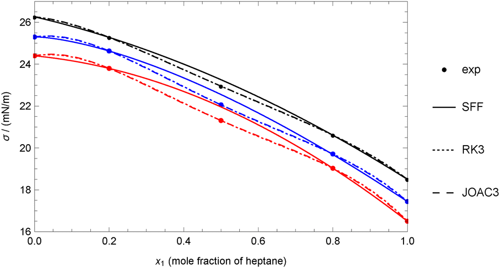
The behavior of both the EBE and CW models for this mixture is shown in Fig. 1 at four different temperatures. Data from two different sources,^61,62 are available but do not agree well. The data from each source were fitted separately. As shown in the inset figure, at 303.15 K, the CW model does not behave properly at the highest mole fraction values, failing to avoid the asymptotic value when considering the data from Rolo et al. This issue is not apparent in the main figure, but it is clear that the data trend is not suitable in this mole fraction range. Nevertheless, the CW model performs well for the other data available at the same temperature, as well as for all other temperatures. In general, the EBE model with a single adjustable coefficient can accurately reproduce the three data points available from ref. 62. On the other hand, the 5 data points from ref. 61 are better represented by the CW model, as the trend is less clear, with the data oscillating around the values predicted by the model.

Fig. 1 Comparison between experimental data and theoretical data for the heptane + decane mixture at different temperatures using experimental data for pure fluids (case 1A). Points: (circle) experimental data of Pugachevich and Belyarov,⁶¹ (diamond) experimental data of Rolo et al.⁶² Colors: (black) 303.15 K, (red) 313.15 K, (green) 323.15 K, (blue) 333.15 K.

As expected, the use of three-adjustable coefficients results in a clear improvement in the correlations, which is not surprising given that, in some cases, the number of fitted data points is fewer than 5. In fact, the mean MAPD values decrease from 0.27 to 0.11 when using the three-coefficient models rather than the two-coefficient models.

Therefore, any of the three-coefficient models considered (RK3, SFF, and JOAC3) can be used accurately. However, it is evident that the SFF model yields the highest deviations, as it can be shown that the value of the coefficient d₃ is restricted to be d₃ ≥ 0, which is not the case for the coefficients in RK3 and JOAC3, making the use of these last preferable. As an example, Fig. 2 shows that the SFF model performs well for heptane + hexadecane at 333.15 K, but it cannot reproduce the experimental value at x = 0.5, as this value appears to be lower than expected. As a result, a non-zero deviation is obtained even though there are only three experimental data points and the model uses three adjustable coefficients. On the other hand, the RK3 and JOAC3 models are more ‘flexible’ and can reproduce all the data perfectly, but they need to deviate from regular behaviour.

Fig. 2 Comparison between experimental data and theoretical data for the heptane + hexadecane mixture at different temperatures using experimental data for pure fluids (case 1A). Experimental data of Rolo et al.⁶² Colors: (black) 313.15 K, (blue) 323.15 K, (red) 333.15 K.

The RK3 and JOAC3 models lead to slightly different values of AADm and PDm. The RK3 model can reproduce all the isotherms with an AAD below 0.65%, while the AADm for the JOAC3 model is 0.8%. However, when considering each data point individually, the JOAC3 model can reproduce all of them with PDs of less than or equal to 1.8%, whereas this value increases to 2.66% for the RK3 model. Considering their analytical form, the RK3 model has the slight advantage of not requiring the use of natural logarithms. Nevertheless, in some situations, RK3 could give negative values (it was not the case for the mixtures considered here), which is an unacceptable result, while JOAC3 always yields positive values.

As mentioned earlier, there are 25 isotherms for which only 3 data points are available (75 data points in total), and another three isotherms with four selected data points (12 data points in total, excluding those for the pure fluids). As explained later, the Akaike criterion cannot be applied to models with three adjustable coefficients when fewer than 5 data points are available for an isotherm, so the isotherms with n = 3 and 4 were discarded in all cases to allow for a meaningful comparison. Therefore, it is interesting to observe the effect of excluding isotherms with 3 or 4 data points from the calculation of the mean deviations. In this particular case, the results obtained in terms of mean deviations are practically the same (files are available upon request). For instance, the maximum difference between including or excluding these isotherms is observed for the JOAC3 model, where the MAPD increases from 0.08% to 0.13%. This suggests that all the isotherms with more than 3 data points are very well reproduced.

4.2.2 Results for case 1B. The results for case 1B, in which the experimental values of the surface tension of pure components are replaced with a model or correlation, are presented in Table 5. The primary objective is to analyze the behavior and performance of the combination of the pure-component correlations with the mixture models, comparing their results to each other and to those previously obtained in case 1A.

Table 5 Calculated deviations for case 1B. MAPD was obtained for 69 isotherms, MPD for 466 data, AADmax for a given isotherm, and PDm for a given datum

MODEL	Ncoef	Origin	MAPD (%)	MPD (%)	AADm (%)	PDm (%)	Number of isotherms with AAD ≤
							0.3%	0.5%	0.8%	1%	1.5%	2.0%	>2%
EBE	1	Phys-chem	0.68	0.68	2.06	6.61	13	26	45	56	67	68	1
WSD	1	Phys-chem	0.65	0.66	1.98	6.61	12	30	48	60	66	69
BCRG	1	Phys-chem	0.71	0.71	2.10	6.61	12	26	44	53	67	68	1
JOAC1	1	Emp	0.74	0.81	5.31	12.57
RK2	2	Emp	0.57	0.58	1.77	6.61	17	34	55	60	68	69
FLW	2	Phys-chem	0.64	0.63	1.84	6.61	14	26	48	60	67	69
CW	2	Phys-chem	0.56	0.56	1.50	6.61	16	34	57	61	69	69
QYDH	2	Phys-chem	0.58	0.59	1.88	6.61	15	32	57	61	68	69
JOAC2	2	Emp	0.60	0.62	2.49	6.61
SIGMO	2	Emp	0.67	0.67	1.90	6.61	8	23	46	61	68	69
RK3	3	Emp	0.43	0.42	1.54	6.61	28	43	66	68	68	69
SFF	3	Emp	0.53	0.52	1.98	6.61	20	36	60	62	68	69
JOAC3	3	Emp	0.43	0.43	1.57	6.61	28	42	63	67	68	69

---

As previously explained, in this case, the experimental values for the pure fluids are treated as data rather than input parameters. Consequently, the number of data points considered for each isotherm ranges from 5 to 15, resulting in a total of 466 values.

As in case 1A, the MAPD and MPD results are very similar across the different models. However, as expected, they are higher than those obtained in the previous case. Specifically, the MAPD ranges from 0.43% to 0.74%, whereas the MPDs varies from 0.42% to 0.81%. As in the previous case, the highest percentage deviations are observed when using the JOAC1 model. Specifically, a maximum percentage deviation (PDm) of 12.57% is obtained for methane + ethane at 173.15 K and molar fractions around 0.8. Due to its poor performance, this model must be discarded, and the number of isotherms reproduced with an AAD below a specified threshold is omitted from Table 5.

The remaining models with one adjustable coefficient perform well, achieving MAPD and MPD values of approximately 0.7%. Notably, the WSD model delivers the best results, yielding the lowest MAPD, MPD, and AADm values. Furthermore, it is the only one-coefficient model capable of reproducing 60 isotherms with an AAD ≤ 1% and all isotherms with AAD ≤ 2%. The other two one-coefficient models produce comparable, though slightly inferior, results. As observed, the PDm value for these three models, as well as for all the others (except for JOAC1), consistently takes a value of 6.61%. This is clearly due to the discrepancy between the value obtained using the specific correlation by Mulero et al. and the experimental value for pentane at 323.15 K reported by Mohsen-Nia.¹⁷ This issue is detailed in Table 3 and was previously discussed in Section 4.1.

As a clear example of the good performance of the 1-coefficient models, Fig. 3 shows the results obtained for hexane + octane at 313.15 K. It can be seen that the models reproduce the experimental data accurately, with the highest deviations due to the disagreement between the experimental value provided by Pugachevich and Belyarov⁶¹ and the obtained from Mulero et al. correlation for pure hexane and octane. It must be taken into account that Mulero et al. considered a collection of data in their proposed correlations, so some deviations can be found with respect to some specific experimental results. In any case, at least here the deviations are not higher than 0.6% as shown in Fig. 3b.

Fig. 3 Comparison between experimental and calculated values of surface tension for hexane + octane at 313.15 K (a) and values of PD(%) (b) considering case 1B. Experimental values of Pugachevich and Belyarov.⁶¹

The results obtained with correlation models using two adjustable coefficients show that RK2, CW, and QYDH yield the best performance, with MAPDs and MPDs below 0.6% and AADs below 1.9%. For these three correlations, no significant differences are observed in the distribution of isotherms with AADs below a specified threshold. For instance, all three models are able to reproduce data for at least 60 isotherms with AADs of 1% or lower. It is worth to mention that the CW correlation achieves the lowest AADm value (1.5%), but in the particular case of the pentane + heptane mixture at 323.15 K, the adjustable coefficient takes a value a = 0.9… (with 15 nines after the decimal point) to avoid the vertical asymptote.

The FLW and SIGMO models perform well, but their results are slightly worse than those of the three models mentioned earlier, and similar to those obtained from some one-coefficient models. For example, the SIGMO model can reproduce only 8 isotherms with AAD ≤ 0.3%, while certain one-coefficient models can reproduce 12 or 13 isotherms with the same AAD threshold.

The highest AADm (2.49%) was obtained with the JOAC2 model. Although this model provides adequate results, it does not offer an improvement compared to the others. As a result, the number of isotherms reproduced with AAD values below a specified threshold is not included in Table 5.

When using three adjustable coefficients, the SFF model yields slightly worse results than the RK3 and JOAC3 models. While the MAPD and MPD values obtained with these three models are lower than those using one or two adjustable coefficients, the decrease is not so important. It is important to note that, in this case, only five data points are considered for some isotherms, which are fitted using three adjustable coefficients.

When comparing the best correlation models using one adjustable coefficient with those using two or three, it is evident that the improvement in MAPDs and MPDs is modest. In all cases, these deviations remain low, always below 1%. On the other hand, as expected, models with a higher number of adjustable coefficients can reproduce a greater number of isotherms with AADs below a specified threshold. For instance, the WSD correlation reproduces 48 isotherms with an AAD ≤ 0.8%, while the CW and QYDH models with two coefficients reproduce 57, and the RK3 correlation reproduces 66.

For pentane + hexadecane a PDm of 6.52% is obtained for all the correlations, which is due to the disagreement between the experimental value for pure pentane at 323.15 K reported by Mohsen-Nia¹⁶ and the obtained by using the specific correlation by Mulero et al.,⁷⁴ as it is shown in Table 3. In fact, this datum was eliminated for the data set used by Mulero et al. to obtain the proposed correlation, as it was in clear disagreement with the rest of the available data at similar temperatures.

When comparing cases 1A and 1B, the general trends remain consistent, with MAPD and MPD yielding similar values and the model fit improving as the number of adjustable coefficients increases from one to two or three. Although the overall accuracy shows a slight decrease, the impact remains minimal, with deviations consistently staying below 1%. Therefore, using the correlations of Mulero et al. for pure compounds in models for mixtures is a reliable approach when experimental data are unavailable, as it does not significantly affect the performance of these models. This method provides a practical solution in cases where obtaining experimental data for pure compounds is challenging or expensive, serving as a feasible alternative for precise modeling.

4.3 Results for case 2

In this case, isotherms are included for which experimental data are available for one of the pure fluids but not for the other. One reason for the absence of the surface tension value for one pure fluid is that the mixture measurements were made at a temperature below the triple point temperature of the substance. Another reason, as in the case of the pentane + heptane mixture, is that the surface tension values for one of the pure fluids were measured at temperatures close to those used for the mixture, but not at exactly the same temperature.¹⁷ As seen in Table 2 only four mixtures are included, with a total of 6 isotherms. Unfortunately, the number of data points available for each isotherm, including the value for one of the pure fluids, ranges from 3 to 5, except for the pentane + heptane mixture, which has nine values.

Two different sub-cases are considered here. In case 2A, the specific correlations proposed by Mulero et al.⁷⁴ are applied to one of the fluids, whereas in case 2B, they are used for both fluids. It is important to note that these specific correlations are valid only within a fixed temperature range. Therefore, in cases where the isotherm is below the triple point of one of the fluids, the specific correlation must be used to obtain an extrapolated value, which, of course, cannot be directly compared with experimental data. The coefficients used to apply these correlations can be found in the ESI.†

4.3.1 Case 2A. As illustrated in Table 2, this case includes only four mixtures and six isotherms. Specifically, three isotherms are considered for the pentane + heptane mixture, each containing eight data points. For the remaining mixtures, a single isotherm is considered, with 3 to 5 data points corresponding to different molar fraction values. The experimental values for pure decane, heptane, and pentane are used as input parameters for each model.

For pure docosane and tetracosane, the isotherms considered fall below either the triple-point temperature reported by DIPPR⁷⁵ or the minimum temperature specified in the correlations provided by Mulero et al.⁷⁴ Despite this, these correlations are utilized, and the resulting values should be regarded as extrapolated. While they cannot be compared to experimental data, they remain valuable for the application of the models considered in this study.

The summary of results of this case is shown in Table 6.

Table 6 Calculated deviations for each correlation model in case 2A. MAPD was calculated for 6 isotherms and MPD for 36 data points for the models with one or two adjustable coefficients. The AADm was obtained for a given isotherm, and the PDm for a given data point

MODEL	Ncoef	Origin	MAPD (%)	MPD (%)	AADm (%)	PDm (%)	Number of isotherms with AAD ≤
							0.3%	0.5%	0.8%	1%	1.5%
EBE	1	Phys-chem	0.52	0.45	1.28	2.98	3	4	4	5	6
WSD	1	Phys-chem	0.45	0.39	0.98	2.98	2	4	5	6	6
BCRG	1	Phys-chem	0.54	0.47	1.36	3.16	3	4	4	4	6
JOAC1	1	Emp	0.46	0.39	0.88	2.77	3	4	5	6	6
RK2	2	Emp	0.24	0.24	0.44	0.99	5	6	6	6	6
FLW	2	Phys-chem	0.27	0.25	0.47	1.74	4	6	6	6	6
CW	2	Phys-chem	0.25	0.25	0.57	2.13	5	5	6	6	6
QYDH	2	Phys-chem	0.23	0.24	0.36	1.11	4	6	6	6	6
JOAC2	2	Emp	0.24	0.24	0.50	0.92	5	6	6	6	6
SIGMO	2	Emp	0.36	0.32	0.66	1.09	4	5	6	6	6
RK3	3	Emp	0.08	0.09	0.25	0.77
SFF	3	Emp	0.13	0.15	0.25	0.78
JOAC3	3	Emp	0.08	0.10	0.24	0.77

---

As observed, all the one-coefficient models provide satisfactory overall results, with MAPDs around 0.5%, and with the JOAC1 and WSD models performing slightly better than EBE and BCRG. The MPD values are slightly lower than the MAPDs, and the highest PDm (3.16%) is obtained by using the BCRG model for the decane + docosane mixture at 313.15 K and x = 0.8.¹⁵ The other three models with one adjustable coefficient produce similar PDm values (near 3%). As can be seen in Fig. 4, the experimental value for pure decane deviates from the trend exhibited by the values at lower molar fractions. Then the highest AADs are associated with the decane + docosane mixture. From a practical point of view, it must be noted that both BCRG and JOAC1 contain logarithms in their analytical expressions, which does not seem to influence the results. In contrast, it can mean slightly more difficult mathematical management.

Fig. 4 Comparison between experimental and calculated values of surface tension for decane + docosane at 313.15 K considering case 2A. Experimental data of Queimada et al.¹⁵ (a) Models with one adjustable coefficient. (b) Models with two adjustable coefficients. (c) Models with three adjustable coefficients.

When two coefficients are considered, the MAPDs and MPDs are reduced to approximately half of those obtained with the one-adjustable coefficient models. The highest deviations are observed with the SIGMO model, whereas the CW model yields the highest PDm value, which is found again for the decane + docosane mixture. The main difference between the CW model and the other models lies in its lower “flexibility”, which prevents it from accurately capturing the different behaviors of the data at high and low molar fractions. In contrast, the other models reproduce well both of these molar fraction ranges, although they might exhibit an “artificial” curvature.

In the case of three adjustable coefficients, the highest AAD value is 0.25%, while the highest PDm is 0.78%, both corresponding to the pentane + heptane mixture at 298.15 K. In general, the obtained MAPDs are approximately half of those found in the case of two-coefficient models. It is important to note that for the heptane + docosane mixture, only three data points are available (in addition to the pure heptane data). Overall, the SFF model is slightly less accurate than the RK3 and JOAC3 models. However, as illustrated in Fig. 4, when the number of data points is low, the RK3 and JOAC3 models do not perform well at both low and high mole fractions. This behavior arises because these models attempt to simultaneously reproduce all available data at intermediate mole fractions while also matching the experimental or predicted values for the pure components.

When mixtures with only 3 or 4 data points are excluded, the number of isotherms is reduced to 4, and the total number of data points decreases to 29. For one-coefficient models, the MAPD values are lower than when all isotherms are considered, ranging from 0.31% to 0.45%, with the JOAC1 model yielding the lowest value. In the case of two-coefficient models, the MAPD values are very similar, with the lowest value (0.22%) obtained for the CW model. Similarly, the reduction to 4 isotherms has only a slight effect on three-coefficient models, yielding MAPD values of 0.11% for RK3 and JOAC3, and 0.19% for SFF. Since the decane + docosane mixture is excluded, the AADm and PDm values are lower than when it is included. However, the overall analysis remains largely unaffected by whether 4 or 6 isotherms are considered.

4.3.2 Case 2B. In this case, the values for the surface tension of both pure fluids are taken from the specific correlations proposed by Mulero et al.⁷⁴ The number of data points considered for each isotherm ranges from 4 to 9, with a total of 42 values across six isotherms. Results are shown in Table 7.

Table 7 Calculated deviations for each correlation model in case 2B. MAPD was calculated for 6 isotherms, MPD for 42 data points, AADm for a given isotherm, and PDm for a given data point

MODEL	Ncoef	Origin	MAPD (%)	MPD (%)	AADm (%)	PDm (%)	Number of isotherms with AAD ≤
							0.3%	0.5%	0.8%	1%	1.5%	2.0%
EBE	1	Phys-chem	1.01	1.05	2.02	5.35	0	1	2	4	5	5
WSD	1	Phys-chem	0.93	0.99	1.99	5.34	0	0	3	5	5	6
BCRG	1	Phys-chem	1.03	1.08	2.03	5.36	0	1	2	3	5	5
JOAC1	1	Emp	0.95	1.00	2.01	5.35	0	0	3	5	5	5
RK2	2	Emp	0.72	0.79	1.68	5.34	1	2	5	5	5	6
FLW	2	Emp	0.69	0.71	1.31	5.34	0	1	5	5	6	6
CW	2	Phys-chem	0.53	0.54	0.87	5.34	1	3	5	6	6	6
QYDH	2	Phys-chem	0.75	0.84	1.82	5.34	1	3	4	5	5	6
JOAC2	2	Emp	0.74	0.81	1.72	5.34	0	2	5	5	5	6
SIGMO	2	Emp	0.86	0.91	1.85	5.34	0	1	3	5	5	6
RK3	3	Emp	0.51	0.57	1.31	5.34	2	5	5	5	6	6
SFF	3	Emp	0.48	0.52	1.01	5.34	1	4	5	5	6	6
JOAC3	3	Emp	0.52	0.58	1.34	5.34	2	4	5	5	6	6

---

The PDm values, around 5.3%, are primarily due to discrepancies between the experimental values provided by Mohsen-Nia et al.¹⁷ for pentane + heptane at 318.15 K (x₁ = 0.971 or x₁ = 1). As shown in Table 3, the values reported by these authors for pure pentane at temperatures around 320 K^16,17 do not align well with those from the Mulero et al. specific correlation. This indicates that these experimental values also differ from those obtained by other authors using experimental or estimation methods, as can be seen in ref. 74.

The MAPDs and MPDs obtained for the models with one adjustable coefficient are around 1%, while the AADms are around 2%. These deviations are nearly double when compared with those observed in case 2A. Nevertheless, the results from these simple models can be considered highly adequate. Specifically, the WSD and JOAC1 models successfully reproduce 5 out of the six isotherms with AADs ≤ 1%, with the only exception being the pentane + heptane mixture at 318.15 K, as previously explained.

When considering two-coefficient models, it is clear that the CW one provides the best overall results. It is the only model that yields both an MAPD and an MPD below 0.55%, and it successfully reproduces all the isotherms with AADs ≤ 1%. In fact, it delivers results that are comparable to, or even better than, those obtained with the three-coefficient models.

As previously explained, the Akaike criterion cannot be applied to three-coefficient models when only four data points are available for an isotherm. This is the case for the heptane + docosane isotherm at 313.15 K, which contains just 4 data points.¹⁴ If these data points are excluded from the calculations, the MAPD and MPD values shown in Table 7 increase slightly. The largest increase is observed for the BCRG model, where the MAPD rises from 1.03% to 1.16%. However, the overall analysis and conclusions remain unaffected by the inclusion or exclusion of these 4 data points.

In general, comparing case 2A with case 2B reveals that the results in the latter are influenced by the discrepancies between the correlation and the experimental values for certain pure fluids. Nonetheless, it has been demonstrated that using the CW model for mixtures in combination with the Mulero et al. model for pure fluids allows for the reproduction of all isotherms with AADs below 0.9%. Moreover, the PD values remain below 5.4%, which can be considered not excessively high.

4.4 Results for case 3

In this case, no available values exist for the two pure fluids in the mixture. Therefore, the specific correlations proposed by Mulero et al.⁷⁴ must be used to obtain these values. As shown in Table 2, this case includes seven mixtures and 39 isotherms, for which 3 to 5 data points are available, resulting in 137 surface tension values. It is important to note that for hexadecane + octacosane and dodecane + hexadecane, only three data points are available for each temperature (16 and 12 isotherms, respectively).^26,67 Consequently, in these cases, models with three adjustable coefficients reproduce the data without deviations.

The summary of the results obtained with each model for case 3 is presented in Table 8.

Table 8 Calculated deviations for each correlation model in case 3. MAPD was calculated for 39 isotherms, MPD for 137 data points, AADm for a given isotherm, and PDm for a given data point

MODEL	Ncoef	Origin	MAPD (%)	MPD (%)	AADm (%)	PDm (%)	Number of isotherms with AAD ≤
							0.3%	0.5%	0.8%	1%	1.5%	2.0%	>2%
EBE	1	Phys-chem	0.63	0.60	1.41	2.95	11	16	24	30	39
WSD	1	Phys-chem	0.60	0.57	1.21	3.43	10	18	26	34	39
BCRG	1	Phys-chem	0.69	0.65	1.26	2.94	9	15	23	29	39
JOAC1	1	Emp	0.69	0.65	2.06	4.66	9	17	23	31	37	38	1
RK2	2	Emp	0.33	0.31	1.06	3.17	22	30	35	38	39
FLW	2	Emp	0.45	0.42	1.36	4.06	22	26	31	33	39
CW	2	Phys-chem	0.35	0.32	1.08	2.90	22	29	33	38	39
QYDH	2	Phys-chem	0.35	0.33	0.93	2.79	21	27	36	39
JOAC2	2	Emp	0.37	0.34	1.34	4.01	20	28	34	38	39
SIGMO	2	Emp	0.50	0.47	1.20	3.23	12	19	33	35	39
RK3	3	Emp	0.04	0.05	0.36	1.04
SFF	3	Emp	0.13	0.13	0.61	1.24
JOAC3	3	Emp	0.04	0.06	0.38	1.10

---

The one-coefficient models yield MAPDs and MPDs in the range of 0.6%–0.7%, with MPDs being slightly lower. Among them, the WSD model provides the best overall performance, accurately reproducing 34 out of 39 isotherms with AADs ≤ 1%. However, it should be noted that this model gives a PDm value of 3.43% for hexadecane + octacosane at 573.2 K and x₁ = 0.84,²⁶ as shown in Fig. 5. The PDm values for EBE and BCRG are slightly below 3%. On the other hand, the JOAC1 model is the only one-coefficient model that fails to reproduce all isotherms with AADs below 1.5%. Nevertheless, as shown in Fig. 5 it produces a PDm value of 4.66% for hexadecane + octacosane, which is significantly higher than those obtained with the other one-coefficient models.

Fig. 5 PD(%) for hexadecane + octacosane mixture at 573.2 K considering case 3 and different correlation models. Experimental data are those by Yang and Wu.²⁶ (a) Models with one adjustable coefficient. (b) Models with two adjustable coefficients.

Regarding the two-coefficient models, SIGMO yields results only slightly better than those obtained with the one-coefficient models. Specifically, it reproduces only 12 isotherms with AADs ≤ 0.3%, whereas the other models of this type achieve this for at least 20 isotherms. Nonetheless, the SIGMO model can reproduce all isotherms with AADs ≤ 1.5%, suggesting that it maintains a reasonable level of accuracy. Surprisingly, JOAC2 and FLW models produce PDm and AADm values comparable to those obtained with the one-coefficient models, specifically for the hexadecane + octacosane mixture (see Fig. 5). The best performance is achieved with the RK2, CW, and QYDH models, which produce lower PDm values and accurately reproduce at least 38 out of the 39 available data points with percentage deviations ≤1%. On the other hand, among these models, JOAC2 provides the poorest fit when considering the other fitting indicators.

In relation to this case, it is important to highlight that the values of a in the CW model must not approach exactly 1 to avoid the appearance of a vertical asymptote. In this regard, four mixtures are identified where attention must be paid to this mathematical condition: (i) heptane + undecane at 333.15 K and 373.15 K, where the value is 0.9… (with 14 nines after the decimal point) and 0.9… (with 20 nines after the decimal point), respectively; (ii) hexadecane + octacosane at 372.76 K, 398.44 K, 423.04 K, and 448.17 K, where the value is 0.9… (with 12 nines after the decimal point) at the first temperature and 0.9… (with 20 nines after the decimal point) at the remaining temperatures; (iii) hexadecane + undecane at 373.15 K, where a is 0.9… (with 20 nines after the decimal point); and finally, (iv) dodecane + hexadecane at 423.09 K, with a value of 0.9… (with 20 nines after the decimal point).

Since there are 28 out of the 39 isotherms for which only 3 data points are available, the overall percentages obtained using three-coefficient models are very low. Among these, the SFF model produces the poorest results when compared to the RK3 and JOAC3 models. Using the latter two models, the PDm values are ≤1.10% and the MAPD is only 0.04%.

When only the remaining 11 isotherms are considered (i.e., those with 4 or 5 data points), the difference between the three models becomes less significant. In this case, the SFF model yields a result similar to that obtained when all the isotherms are included, while for RK3 and JOAC3, the MAPD increases to 0.13% and 0.14%, respectively. Additionally, it can be confirmed that, when only the nine isotherms with 5 data points are considered, the MAPDs for most models are lower than when all isotherms are included. However, for RK3 and JOAC3, the MAPDs remain the same as when considering the isotherms with 4 and 5 data points.

4.5 Results for case 4

In this case, the temperature of the mixture exceeds the critical temperature of at least one of the pure fluids. Following the approach of other authors,^19,76 the surface tension value at temperatures higher than the critical temperature value, as reported in the DIPPR database,⁷⁵ is considered to be zero. This results in the exclusion of two models: WSD and JOAC. As shown in Table 1, in the case of the WSD model, the fitting coefficient (ϕ₁₂) is multiplied by , and setting σ₁ = 0 or σ₂ = 0, eliminates the fitting capability of the correlation. For the JOAC model, calculating the natural logarithm of zero is not possible.

All the mixtures considered in this case contain methane, whose critical point is around 190.6 K.^74,75 The other components are ethane, propane, pentane, nonane, and decane, with data taken from ref. 63 and 68–72, as shown in Table 2. Since all isotherms considered correspond to temperatures above 190.6 K, the surface tension of methane has been assumed to be zero in all models. This assumption serves as a first approximation and it means to setting σ₁ = 0 in all the models analyzed, which means that the surface tension of the mixture will be zero only when x₁ = 1. From a strict theoretical perspective, the surface tension of the mixture should vanish at a critical molar fraction x_c < x₁, which cannot be determined using correlation models, as it requires an equation of state and/or other approaches.³⁶

As shown in Table 2, this case includes five mixtures, with a total of 21 isotherms and 158 data points. As in previous cases, two approaches are considered: case 4A, which uses the experimental value for one of the pure fluids, and case 4B, which employs the surface tension value predicted by the correlations proposed by Mulero et al.⁷⁴ Each case is analyzed separately in the following subsection.

4.5.1 Results for case 4A. Only two mixtures are considered in this case. For methane + propane there are data available for five temperatures from ref. 68 and three additional temperatures from ref. 69. In the latter case, the measurements were taken at slightly different temperatures for each molar fraction, so the temperature values reported in Tables 2 and 3 represent mean values. The total number of data points for this mixture (excluding the values for pure propane) is 65. For methane + ethane, measurements are available at six temperatures, including values for pure ethane.⁶³ Excluding the data for pure ethane, the total number of data points considered here is 34.

The results for these two mixtures, which include 14 isotherms and 99 data points, are presented in Table 9. As observed, the MPD values are generally higher than the MAPD values. This is primarily because the number of data points for each isotherm ranges from 3 to 12. Additionally, the results for the methane + propane mixture are noticeably worse, exhibiting higher percentage deviations overall compared to those for the methane + ethane mixture.

Table 9 Calculated deviations for each correlation model in case 4A. MAPD was calculated for 14 isotherms, MPD for 99 data points, AADm for a given isotherm, and PDm for a given data point. Sections (a) and (b) show the results separately for the two mixtures considered in this case. (a) Results for methane + propane. MAPD was calculated for 8 isotherms, MPD for 65 data points. (b) Results for methane + ethane. MAPD was calculated for 6 isotherms, MPD for 34 data points

Model	Ncoef	Origin	MAPD (%)	MPD (%)	AADm (%)	PDm (%)
EBE	1	Phys-chem	21.3	23.8	46.3	284.2
BCRG	1	Phys-chem	27.9	31.0	56.8	325.6
RK2	2	Emp	1.6	1.8	4.2	13.8
FLW	2	Emp	21.2	23.8	46.3	284.2
CW	2	Phys-chem	1.6	1.8	4.2	14.6
QYDH	2	Phys-chem	8.4	9.5	20.3	105.2
SIGMO	2	Emp	8.9	10.2	21.3	111.4
RK3	3	Emp	1.3	1.5	4.2	12.9
SFF	3	Emp	2.0	2.1	4.7	15.7

---

(a)
EBE	1	Phys-chem	34.2	34.0	46.3	284.2
BCRG	1	Phys-chem	44.6	44.5	56.8	325.6
RK2	2	Emp	2.3	2.3	4.2	13.8
FLW	2	Emp	34.1	33.9	46.3	284.2
CW	2	Phys-chem	2.3	2.3	4.2	14.6
QYDH	2	Phys-chem	13.7	13.8	20.3	105.2
SIGMO	2	Emp	14.6	14.7	21.3	111.4
RK3	3	Emp	1.8	1.9	4.2	12.9
SFF	3	Emp	2.8	2.8	4.7	15.7

---

(b)
EBE	1	Phys-chem	4.1	4.4	7.6	13.7
BCRG	1	Phys-chem	5.6	5.9	9.4	15.9
RK2	2	Emp	0.6	0.8	1.4	4.2
FLW	2	Emp	4.1	4.4	6.5	13.7
CW	2	Phys-chem	0.7	0.8	1.4	4.2
QYDH	2	Phys-chem	1.3	1.5	2.2	4.8
SIGMO	2	Emp	1.4	1.6	2.4	6.4
RK3	3	Emp	0.5	0.7	1.2	3.6
SFF	3	Emp	0.8	0.9	1.5	4.6

---

Table 9(a) and (b) present the results for the two mixtures separately. As shown in Table 9(a), the models with one adjustable coefficient are inadequate for reproducing the available data for the methane + propane mixture, no matter the source of data used (ref. 68 and 69). Thus, the MAPD values exceed a 34% and PDm values greater than 284%. It is not surprising to obtain percentage deviations greater than 100% when the surface tension takes values very near to zero, because even a small absolute deviation results in a large percentage deviation.⁷⁴ Nevertheless, as it is shown in Table 9(a), there are other models that can reproduce all the data with clearly lower percentage deviations.

Notably, the highest PDm values are observed for this mixture at 303.15 K and a mole fraction of 0.452, which corresponds to the highest mole fraction at which surface tension measurements were taken.⁶⁸ As a clear example, Fig. 6a shows the results obtained at 303.15 K, compared with the measurements performed by Weinaug and Katz.⁶⁸ It is evident that the EBE and BCRG models fail to reproduce the data trend. The same applies to the FLW, QYDH, and SIGMO 2-coefficient models, where the isotherms follow a trend completely different from the data and even exhibit inflection points. In contrast, the RK2 and CW models accurately reproduce this isotherm, while the 3-coefficient models provide similar results with no clear improvement over the previous ones.

Fig. 6 Comparison between experimental and calculated values (lines) of surface tension for methane + propane mixture at 303.15 K considering case 4A. Experimental data of Weinaug and Katz.⁶⁸ (a) Models with one adjustable coefficient. (b) Models with two adjustable coefficients. (c) Models with 3 adjustable coefficients.

The results for the methane + ethane mixtures are different than those for methane + propane. Thus, as can be seen in Table 9(b), for the two 1-coefficient models, the MAPDs are 4.1% and 5.6%, respectively. These values can be considered as high when compared to those obtained with models containing two adjustable coefficients.

Regarding the overall results obtained with the two-coefficient models, it is worth noting that, surprisingly, the FLW model yields results nearly identical to those of the EBE one with just one adjustable coefficient. This occurs because one of the coefficients in the FLW model takes on an extremely high or low value, effectively making zero one of the terms in the model.

On the other hand, the CW and RK2 models are able to reproduce the data for the two mixtures with PDs of 14.6% or lower and AADs of 4.3% or lower. In the application of the CW model, it must be taken into account that for the methane + ethane mixture at 253.15 K, the adjustable coefficient must take a value a = 0.9… (with 20 nines after the decimal point) in order to avoid the vertical asymptote.

Surprisingly, the SFF model, despite having three adjustable coefficients, does not yield better results than the two previously mentioned, while the RK3 model only slightly improves the results compared to CW or RK2.

For the QYDH and SIGMO models, the obtained results differ significantly for each mixture and fail to reproduce the surface tension behavior of methane + propane, at least within the temperature and molar fraction ranges where data are available. Better results are obtained for methane + ethane, but with significantly higher deviations than those offered by other models.

For the methane + propane mixture, all isotherms have five or more data points. In contrast, for the methane + ethane mixture, there are three isotherms with fewer than five surface tension values available. A total of 23 data points are available for the remaining three isotherms. When only these latter isotherms are considered, the MAPD and MPD values obtained are slightly higher than when all isotherms are included. For example, in the case of the RK2, CW, and RK3 models, the MAPD increases from around 0.6% to approximately 0.9% (this can be checked using the data provided in the ESI†). However, this slight increase does not alter the main conclusions, particularly the fact that some models consistently perform better than others.

4.5.2 Results for case 4B. In this case, the surface tension value for the second component of the mixture is obtained using the correlation proposed by Mulero et al.⁷⁴ This analysis includes the five mixtures labeled as case 4 in Table 2, considering a total of 21 isotherms and 158 data points. However, these data are not homogeneously distributed, as the number of data points per isotherm ranges from 3 to 13. Consequently, the MAPD values are lower than the MPD ones.

The overall results for this case are presented in Table 10. As shown, MAPDs in the range of 15%–20% and percentages exceeding 280% are obtained for the five mixtures when using one-coefficient models. These high deviations stem from the fact that the models, which assume a surface tension of zero for methane, fail to adequately predict the available data for two of the mixtures: methane + propane and methane + pentane, as shown in Table 10(a). In contrast, as seen in Table 10(b), the situation is markedly different for the other three mixtures. Both the EBE and BCRG models can reproduce the data at least qualitatively, yielding significantly lower percentage deviations than those observed for the methane + propane and methane + pentane mixtures. Specifically, for the latter three mixtures, the MAPDs obtained with one-coefficient models fall within the range of 3%–4%, whereas for the other two mixtures, they increase to 26%–35%.

Table 10 Calculated deviations for each correlation model in case 4B. MAPD was calculated for 21 isotherms, while MPD was determined from 158 data points. AADm corresponds to a given isotherm, and PDm to a given data point. Sections (a) and (b) present the results separately for the different mixtures considered in this case. (a) Results for methane + propane, and methane + pentane. MAPD was calculated for 11 isotherms and MPD for 102 data. (b) Results for methane + ethane, methane + nonane, and methane + decane. MAPD was calculated for 10 isotherms and MPD for 56 data

MODEL	Ncoef	Origin	MAPD (%)	MPD (%)	AADm (%)	PDm (%)	0.5%	1%	2%	3%	5%
EBE	1	Phys-chem	15.4	17.8	40.5	284.1
BCRG	1	Phys-chem	20.0	23.3	52.5	325.6
RK2	2	Emp	1.7	2.0	5.5	18.8	5	8	16	18	19
FLW	2	Emp	15.1	17.6	40.5	284.1
CW	2	Phys-chem	1.9	2.2	5.5	18.7	3	6	13	17	19
QYDH	2	Phys-chem	6.5	7.8	18.5	105.2
SIGMO	2	Emp	7.4	8.5	19.7	111.0
RK3	3	Emp	1.5	1.8	4.2	14.4	6	9	15	18	21
SFF	3	Emp	1.8	2.1	6.5	16.3	5	8	14	17	19

---

Model	Ncoef	Origin	MAPD (%)	MPD (%)	AADm (%)	PDm (%)
(a)
EBE	1	Phys-chem	26.5	25.7	40.5	284.1
BCRG	1	Phys-chem	34.6	33.7	52.5	325.6
RK2	2	Emp	2.6	2.8	5.5	18.8
FLW	2	Emp	26.3	25.5	40.5	284.1
CW	2	Phys-chem	2.7	2.8	5.5	18.7
QYDH	2	Phys-chem	11.5	11.4	18.5	105.2
SIGMO	2	Emp	12.3	12.2	19.7	111.0
RK3	3	Emp	2.4	2.5	4.2	14.4
SFF	3	Emp	2.9	2.9	6.5	16.3

---

(b)
EBE	1	Phys-chem	3.2	3.5	6.4	13.5
BCRG	1	Phys-chem	3.9	4.4	8.1	16.0
RK2	2	Emp	0.6	0.7	1.5	4.3
FLW	2	Emp	2.8	3.3	6.4	13.5
CW	2	Phys-chem	1.1	1.0	3.3	6.6
QYDH	2	Phys-chem	0.9	1.1	2.0	4.6
SIGMO	2	Emp	2.0	1.8	7.6	12.3
RK3	3	Emp	0.5	0.6	1.2	3.6
SFF	3	Emp	0.6	0.7	1.6	4.5

---

As in case 4A, the FLW model yields practically the same results as the EBE model, despite having an additional adjustable coefficient. This holds for all mixtures except, surprisingly, methane + decane. This discrepancy may be attributed to the limited availability of experimental data for this mixture, as only three data points are available for two of the considered temperatures.

The RK2 and CW models yield the best results when using two coefficients. In particular, the RK2 model performs slightly better, even surpassing the three-coefficient SFF model. Both RK2 and CW can reproduce all the isotherms with AADm ≤ 5.5%, with the highest deviations observed for the first two mixtures (see Table 10(a)). Furthermore, RK2 accurately reproduces the data for the three mixtures listed in Table 10(b).

As an example of the excellent performance of the RK2 model, the results for methane + ethane at three temperatures are shown in Fig. 7. As can be seen, the predictions for pure ethane align very well with the experimental data. It is evident that using only one adjustable coefficient, as in the RK1 model, is insufficient to reproduce the data trend, while using two coefficients accurately yields excellent results, particularly at low temperatures. In fact, the results obtained with RK3 do not show significant improvements over those from RK2.

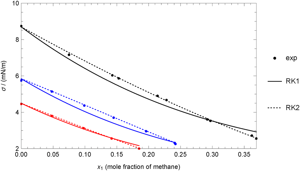Fig. 7 Comparison between experimental data and correlations for the methane + ethane mixture at different temperatures using correlation data for ethane. Points: (circle) experimental data of Baidakov et al.⁶³ Colors: (black) 233.15 K, (blue) 253.15 K, (red) 263.15 K.

In the application of CW model it must be taken into account that the adjustable coefficient a takes a value very near to 1 (with a lot of nines after 0.9) in the following cases: methane + ethane at 253.15 K, methane + nonane at 294.26 K, and methane + decane at 277.59 K, 310.93 K, and 344.26 K.

The FLW, QYDH, and SIGMO models fail to adequately reproduce the data for the methane + propane and methane + pentane mixtures, with MAPDs exceeding 11%. However, the situation differs for the other three mixtures. Specifically, the QYDH model accurately reproduces the 11 isotherms for methane + ethane, methane + nonane, and methane + decane, as shown in Table 10(b).

As expected, the RK3 model yields the lowest deviations, although these are not significantly lower than those obtained with RK2. Moreover, it should be noted that for two isotherms, only three data points are available, and the RK3 model uses three adjustable coefficients.

When comparing with case 4A, and considering that the number of data and isotherms selected are different, it can be observed that the MAPD and MPD values are of the same order. This indicates that the use of the Mulero et al. correlations does not significantly affect the obtained results, making it a clear option when data for pure fluids in a binary mixture are unavailable.

In this case, there are four isotherms for which only 3 or 4 data points are available, and therefore, they cannot be included in the analysis based on the Akaike information criterion. Specifically, one of the isotherms corresponds to 273.15 K for methane + ethane, and the other three correspond to methane + decane. If these four isotherms are excluded from the calculation of the MAPD and MPD, the values are based on 17 isotherms and 144 data points. As a result, the MAPD for RK2 increases from 1.6% to 2.0%, and the MPD rises from 2.0% to 2.2%. For RK3, the MAPD increases from 1.5% to 1.8%, while the MPD rises from 1.8% to 2.0% (this can be checked using the data provided in the ESI†). Therefore, the inclusion or exclusion of these data points does not significantly affect the previous analysis of the results.

4.6 Model comparison and evaluation using Akaike criterion

Additionally to the previous results, the corrected Akaike information criterion (AICc) has been used to select the model that in overall best balances goodness of fit and complexity. Unlike the standard Akaike information criterion (AIC), the AICc includes an additional correction term to account for small sample sizes, specifically when the ratio of the number of data points (n) to the number of adjustable coefficients (k) is less than 40, which applies to all models considered in this study. This correction helps to prevent overfitting by penalizing models with an excessive number of coefficients relative to the sample size.^38,39

In this study, the AICc was calculated for the 13 evaluated models without distinguishing between cases 1 to 3. Case 4 was initially excluded due to the high deviations observed in some models. This exclusion is particularly justified by the fact that one of the components in case 4 is in a supercritical state. Since all models assume that surface tension reaches zero only at x₁ = 1, they cannot account for the possibility that the mixture's surface tension may vanish at a lower, critical mole fraction. As a result, their predictions in this case may systematically overestimate the surface tension near this region. Additionally, as explained above, some models cannot be applied to case 4 because their equations simplify to a point where their application is no longer meaningful. In any case, case 4 is considered separately at the end of this section.

Therefore, in this AICc-based comparison, the isotherms from cases 1, 2, and 3 were analyzed, resulting in a total of 128 isotherms per model, corresponding to 819 data points in total. Please note that isotherms with n = 3 and n = 4 were excluded, as they prevented the calculation of AICc according to eqn (7). Despite the exclusion of certain isotherms, this analysis still considers a significant number of data points and isotherms across different cases, allowing for a global evaluation of each model's performance.

Once the AICc values were calculated for each model, the minimum AICc (AICc_min) was determined by selecting the smallest value among them. Then, the relative differences (ΔAICc = AICc − AICc_min) were calculated for each model. This approach normalizes the AICc values, ensuring that the best-fitting model has a value of 0, which simplifies the comparison of the performance of other models relative to the best one. The results for cases 1, 2 and 3 are presented in Fig. 8.

Fig. 8 Corrected Akaike information criterion (AICc) results for the global analysis of cases 1, 2, and 3. The figure shows the relative differences (ΔAICc = AICc − AICc_min) for each model. Black, blue, and red bars represent models with one, two, and three adjustable coefficients, respectively.

The model with the lowest ΔAICc, and therefore the most suitable for describing the experimental data considered in this work, is WSD (and then the value ΔAICc = 0.0 was taken as reference). This indicates that WSD provides the best balance between fit quality and complexity, making it the preferred model for predicting surface tension in these binary mixtures. However, as previously mentioned, this model cannot be applied in case 4, where one of the components is in a supercritical state. As a result, the conclusions drawn from the AICc analysis for cases 1, 2, and 3 cannot be directly extended to case 4.

Among the one-coefficient models, WSD is followed by EBE and BCRG, both of which show significantly poorer fits. Since a ΔAICc difference greater than 10 is already considered strong evidence against a model,³⁸ these confirm that EBE and BCRG are much less suitable for describing the experimental data.

For two-coefficient models, CW has the lowest AICc, but its performance is much weaker than that of WSD. Among the three-coefficient models, JOAC3 has the lowest AICc, but its high ΔAICc clearly indicates overfitting, with no improvement in predictive accuracy.

When comparing physicochemical and empirical models, the physicochemical models generally provide better results. The best among them is WSD, which significantly outperforms other models in this category, including EBE, BCRG, CW, and QYDH. Among the empirical models, FLW is the one giving the best results, but its fit still lags behind that of the less precise physicochemical models.

These results show that physicochemical models provide a more accurate description of surface tension in alkane binary mixtures. Additionally, a high number of adjustable coefficients does not necessarily improve prediction, as more complex models tend to overfit the data without offering real benefits. Therefore, the WSD model is the most appropriate and should be preferred in future applications for mixtures without supercritical fluids, while avoiding models with more coefficients that do not significantly improve data fitting.

Importantly, it should be mentioned that if only cases 1B, 2B, and 3 were considered (where pure component data are either nonexistent, in which case the Mulero et al. correlation is used, or, when available, replaced by the same correlation), the AICc results, in terms of the model rankings, are identical to those obtained for cases 1, 2, and 3. This suggests that the use of these correlations is fully appropriate in this context as well.

In the AICc analysis for case 4, 28 isotherms and a total of 232 data points were considered, and the results are shown in Fig. 9. RK3, with a ΔAICc of 0, provides the best fit and is therefore the most suitable model for this case. The models RK2 and CW, with ΔAICc values of 10.7 and 13.3, respectively, show only minor differences from RK3, suggesting they are still reasonable alternatives, as their ΔAICc values slightly exceed the commonly accepted threshold of 10.³⁸ In contrast, a significant increase in ΔAICc is observed for the remaining models, with SFF showing the highest increase, followed by SIGMO, QYDH, EBE, FLW, and BCRG, all of which demonstrate substantially poorer fits.

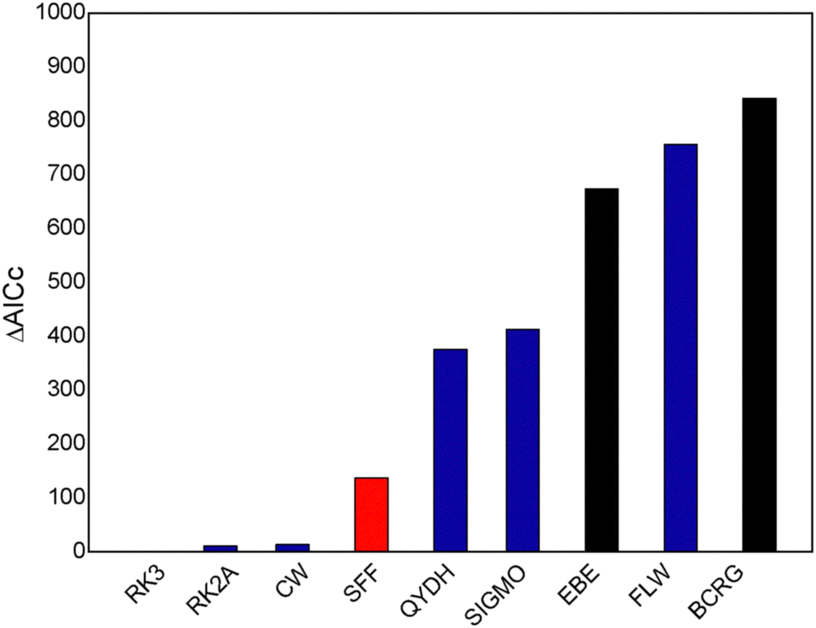Fig. 9 Corrected Akaike information criterion (AICc) results for analysis of cases 4, where one of the pure fluids in the mixture is in a supercritical state. The figure shows the relative differences (ΔAICc = AICc − AICc_min) for each model evaluated. Black, blue, and red bars represent models with one, two, and three adjustable coefficients, respectively.

Regarding the number of adjustable coefficients, among the one-parameter models, BCRG ranks last, while EBE comes third from the bottom, making both the least viable options. Among the two-coefficient models, RK2 and CW yield similar results and perform better than the other two-coefficient models, with their ΔAICc values only slightly higher than that of the best model, RK3. In the case of the three-coefficient models, RK3 stands out as the best, followed by SFF, though at a considerable distance.

When comparing physicochemical and empirical models, it is clear that the empirical models, particularly RK3 and RK2A, provide the best fit in case 4, as indicated by their relatively low ΔAICc values. The physicochemical model CW also performs reasonably well, with a ΔAICc value of 13.3. However, there is a significant increase in ΔAICc values for the remaining physicochemical models, with QYDH showing a notably high value, and even higher values for EBE and FLW, which are within the last three positions in the ranking. From these results, it is suggested that, in general, empirical models are better suited for scenarios involving mixtures with supercritical fluids, at least when the surface tension of the supercritical fluid is considered as zero. However, if a physicochemical model is preferred, CW remains quite a valid alternative.

5 Conclusions

Available data for the surface tension of alkane–alkane binary mixtures have been collected and used to assess the accuracy and applicability of various correlation models from the scientific literature. A total of 803 data points for 26 mixtures have been considered. Based on the availability of data for the pure fluids in the mixtures, four distinct cases have been studied separately. The correlation models use the surface tension of pure fluids and the molar fraction as input data. Four of these models are purely empirical, while the remaining six are based on some physicochemical principles. Since some models include between 1 and 3 adjustable coefficients, a total of 13 different analytical expressions have been evaluated. In cases where the surface tension value for one or both pure fluids was not measured by the same authors who provided the experimental data for the mixture, the correlations proposed by Mulero et al. were used in conjunction with the previously mentioned models for mixtures. Additionally, when the temperature exceeds the critical temperature of one of the mixture components (i.e., when one of the substances becomes a supercritical fluid at that temperature), its surface tension was considered as zero at a plausible approximation.

The accuracy of the models was assessed by calculating the mean absolute percentage deviation (MAPD), the mean percentage deviation (MPD), the maximum absolute percentage deviation (AADm) and the maximum percentage deviation (PDm). These deviations were calculated for each isotherm (i.e., for each set of data obtained for each reference at a fixed temperature for a given mixture), and the mean values across all isotherms were then determined for each case considered.

As expected, when the correlation for pure fluids is used instead of the experimental surface tension values, the deviations negatively impact the overall results, leading to higher deviations. Nevertheless, it has been shown that MAPD and MPD values below 1.1% are achieved even with 1-adjustable-coefficient models when the temperatures considered are below the critical point temperature of both components in the mixture. When one of the components is supercritical, the combination of mixture models and correlations for pure fluids also yields results very similar to those obtained using the experimental values for the pure fluids.

The main conclusions obtained from the analysis of the results obtained with each model are summarized below.

– The JOAC model, which uses the natural logarithms of the surface tension values, does not significantly improve the results compared to the other models where the surface tension is treated as a linear value. Furthermore, this model does not allow for considering the surface tension as zero at temperatures above the critical point temperature of the components in the mixture, as in case 4.

– The BCRG model yields results very similar to those of other one-coefficient models, but it is mathematically more complex due to the presence of logarithms in its analytical expression. Based on the results obtained across all the cases considered, it can be concluded that the use of logarithms is unnecessary, as comparable results can be achieved with simpler analytical expressions, such as those of the EBE or WSD models.

– The WSD model provides very satisfactory results and can be considered the best-performing one-coefficient model when combined with the correlations for pure fluids proposed by Mulero et al. However, the improvement over the analytically simpler EBE model is not substantial. It should also be noted that the WSD model cannot be directly applied when one of the fluids in the mixture is supercritical, i.e., at temperatures above the critical point temperature of one of the components. This is because the only adjustable coefficient appears in the term where the surface tension of the supercritical fluid is considered zero, making it impossible to calculate.

– The EBE model is an analytically simple expression with just one adjustable coefficient, it has some physicochemical basis and it provides excellent results across the various cases considered here. In particular, it accurately reproduces the surface tension of binary mixtures of n-alkanes with MAPDs (calculated for the set of mixtures in each case) below 1% and AADs (calculated for each temperature) below 2.1% when combined with the correlations for pure fluids proposed by Mulero et al. at temperatures below the critical point of both fluids. When the approach of taking the surface tension of the supercritical fluid as zero is applied, the EBE model in combination with Mulero et al. correlation reproduces the data for methane + ethane, methane + nonane, and methane + decane with percentage deviations ≤13.5% and MAPDs slightly higher than in the other cases. This increase in deviations is likely due to the chosen approach rather than the analytical expressions considered.

– The SIGMO model was specifically designed to reproduce isotherms where the curvature of the data changes from concave to convex, or vice versa, which is not the case for the mixtures considered here. However, it is expected to perform well in simpler cases. Our results confirm that it can be used with confidence, yielding low deviations, except when the approach of taking the surface tension of methane as zero is applied to the data for methane + propane and methane + pentane. In particular, the SIGMO model reproduces the data for mixtures with undercritical fluids with MAPDs below 0.9% and ≤2% for mixtures with supercritical methane, except for the two previously mentioned. On the other hand, it is worth noting that, in most of the isotherms considered, the SIGMO model yields slightly higher percentage deviations compared to the other 2-coefficient models. In some cases, the obtained deviations are of the same order as those given by certain 1-coefficient models. Finally, it should be noted that this model includes adjustable exponential coefficients, which can complicate its mathematical handling. In conclusion, while the SIGMO model can be used for these types of mixtures, its application does not lead to a clear improvement over simpler models.

– The analytical expression of the FLW model is slightly more complex than others, as it consists of the sum of three fractions. Additionally, it must be noted that the denominators can approach zero, which would make the model unavailable in such cases. The model behaves similarly to other 2-coefficient models, with MAPDs below 0.7% for cases 1 to 3 (when both fluids are undercritical). However, when one of the fluids is supercritical and the approach of taking its surface tension as zero is used, the FLW model yields results nearly identical to those of the 1-coefficient EBE model, thus making its use less favorable. In conclusion, although this model can be applied with reasonable accuracy in most cases, its greater analytical complexity does not result in improved performance compared to simpler models.

– The QYDH model, based on a physicochemical basis, is specifically designed to reproduce sigmoidal surface tension isotherms in binary liquid mixtures. It incorporates two adjustable coefficients with physical significance, one of which is an exponent. The results obtained with this model are very similar to those provided by SIGMO. Specifically, it yields MAPDs below 0.75% for mixtures in cases 1 to 3, and ≤1.3% for case 4, with the exception of methane + propane and methane + pentane. Given that other 2-coefficient simpler models provide slightly better results, it can be concluded that the use of the QYDH model is not necessary, at least for the n-alkane binary mixtures considered in this study.

– The Redlich–Kister model with two adjustable coefficients (RK2) is purely empirical and delivers excellent results for all the mixtures and cases considered in this study. Specifically, MAPDs below 0.7% are achieved when both fluids are undercritical, while the deviation increases to 1.6% when one of the fluids is supercritical. In this latter case, it performs well, even for mixtures where other models produce clearly incorrect results. In cases 1 to 3, the highest percentage deviations for this model occur when it is used in combination with the Mulero et al. correlations for pure fluids, and the latter deviates significantly from the experimental values. Nevertheless, all data are reproduced with PDs below 6.7%. In case 4B where methane is supercritical, the data for methane + ethane, methane + nonane, and methane + decane are reproduced with PDs below 4.4%, while for methane + propane and methane + pentane, the maximum PDm value is 18.8%. Although this value may seem high compared to the results for other mixtures, it is relatively low when compared to the PDm values obtained with most of the other models considered.

– The CW model is based on certain physicochemical principles, and its analytical expression is relatively simple. However, it contains a denominator that may occasionally approach zero, creating an asymptote that is difficult to avoid. In fact, one of the adjustable coefficients must be set to values very close to 1, requiring an extremely high degree of precision (with many decimal places). In particular, this occurs for 15 isotherms considered in this work. This mathematical issue limits the model's applicability, and caution is necessary during fitting to ensure that asymptotes do not arise. Apart from this, it provides excellent results with MAPDs below 0.6% for cases 1 to 3, comparable to those obtained by the RK2 model. In case 4B, it produces slightly worse results than RK2 for methane + ethane, methane + nonane, and methane + decane. However, the maximum PDm for these mixtures remains relatively low, at 6.6%.

– The SFF model is purely empirical and contains three adjustable coefficients, one of which is an exponent. It generally provides very good results for mixtures without supercritical components, with MAPDs ≤ 0.53%. However, it does not significantly improve the results obtained with some 2-coefficient models, and in general, it yields slightly worse results than other 3-coefficient models. When one of the fluids is supercritical, the MAPDs obtained are slightly higher than those given by some 2-coefficient models. Therefore, it can be concluded that its use is not recommended, at least for the type of mixtures considered here.

– The RK3 model is purely empirical and includes three adjustable coefficients. It provides excellent results for cases 1 to 2, with MAPDs of 0.08% when the experimental surface tension values of pure fluids are used as input data, and a maximum PDm of 2.7%. When the Mulero et al. correlations for pure fluids are used, the MAPDs increase to 0.4–0.5% for cases 1 and 2 and it is very low (0.04%) in case 3 (correlations are used for both pure fluids). In case 4, when the surface tension of methane is considered as zero, the improvement of the RK3 model over the RK2 model is not significant. That is, two adjustable coefficients are sufficient to obtain adequate results, and the inclusion of a third coefficient does not lead to a clear improvement. It is important to note that for some mixtures, only three data points were available, meaning that in those cases, the results obtained with the three-coefficient models are perfect, with zero deviations.

It has to be said that some correlations could be discarded before fitting when the data trend is known. For example, some of the correlations compiled in Table 1 only yield values between the surface tension of the pure components. These correlations cannot be used with isotherms containing data values higher than or lower than those corresponding to the pure fluids. Moreover, some correlations are known to be S-type or L-type; for example, an S-type data trend cannot be fitted accurately using an L-type correlation.

Taking into account all the results, it can be concluded that the use of the correlations proposed by Mulero et al. for pure compounds is a reliable approach when experimental data are unavailable, as it does not significantly affect the performance of the models applied to mixtures. This approach offers a practical solution in situations where experimental data for pure compounds are difficult or costly to obtain, providing a viable alternative for accurate modeling.

According to the results obtained for the averaged deviations, both the WSD and EBE models can be considered the best one-coefficient options, providing excellent results except when one of the fluids is supercritical. Additionally, these models have a certain physicochemical basis. When two coefficients are required to achieve higher accuracy, the RK2 model can be considered the most accurate and suitable option. Other models, including the most recent ones and those with three adjustable coefficients, are not required for binary mixtures of n-alkanes. In particular, the CW model provides good results but may exhibit an asymptote. Unfortunately, the available two-coefficient-physicochemical models cannot be reliably applied to all the cases considered here, and no three-coefficient-physicochemical models have been proposed to date.

Based on the AICc analysis for cases where none of the pure fluids are supercritical, it can be concluded that, among the physicochemical models, WSD provides the best fit, outperforming models such as EBE, BCRG, CW, and QYDH. FLW is the most accurate among the empirical models, though still below the physicochemical models. Additionally, it was found that models with a higher number of adjustable coefficients, such as those with two or three coefficients, do not improve prediction and may lead to overfitting without providing real benefits, with the one-coefficient models offering the best fit. Finally, the use of the Mulero et al. correlations for pure fluids in these specific cases yields identical results in terms of AICc, further validating its application in this context.

In cases where one of the fluids in the mixture is supercritical, the AICc analysis indicates that empirical models, particularly RK3 and RK2, which are based on polynomial equations, provide the best fits. The physicochemical model CW also yielded reasonable fits, comparable to RK2. In contrast, the remaining models perform significantly worse and could be disregarded. In particular, the one-coefficient models have the lowest accuracy, suggesting that models with more coefficients may be better suited for supercritical fluid mixtures.

By combining the deviation analysis and the Akaike criterion, it is concluded that the WSD model is the most suitable for correlating the surface tension of non-supercritical binary mixtures of n-alkanes. It provides the best fit with a single adjustable coefficient and is based on a physicochemical framework. For mixtures containing a supercritical fluid, empirical models based on polynomial expressions, such as RK2 and RK3, offer the best fits. The CW model, which is also based on a physicochemical approach and includes two adjustable parameters, provides reasonable results as well, although its applicability may be limited by the presence of an asymptote.

Author contributions

A. M.: conceptualization, methodology, writing – original draft, writing – review & editing A. H.: software, validation, writing – review & editing V. V. R.: conceptualization, data curation, methodology, writing – original draft, writing – review & editing I. C.: data curation, software, writing – review & editing.

Data availability

Values of the adjustable coefficients and the calculated percentage deviations for each isotherm and model are provided in an Excel file, included in the ESI.† Calculations of the corrected Akaike information criterion are available upon request.

Conflicts of interest

There are no conflicts to declare.

Acknowledgements

This work was supported by funds from the “Junta de Extremadura” and the European Regional Development Fund (ERDF/FEDER) through the project GR24010.

Notes and references

1. H. Wang, D. Luo, E. Velasco, L. Yu and J. Li, J. Mater. Chem. A, 2021, 9, 20874–20896.
2. R. A. Meyers, Handbook of petroleum refining processes, Mc-Graw-Hill, 3rd edn, 2004.
3. D. S. Sholl and R. P. Lively, Nature, 2016, 532, 435–437.
4. J. G. Speight, Handbook of industrial hydrocarbon processes, Gulf Professional Publishing, 2019.
5. A. Dong, J. Phys. Chem. Biophys., 2021, 11, e300.
6. D. Myers, Surfaces, Interfaces, and Colloids: Principles and Applications, John Wiley & Sons, Inc., 1999.
7. J. G. Speight, The chemistry and technology of petroleum, CRC press, 2006.
8. D. Green, G. Willhite, et al., Society of Petroleum Engineers, Richardson, Texas, 1998.
9. A. Dupuy, V. Athes, J. Schenk, U. Jenelten and I. Souchon, J. Membr. Sci., 2011, 378, 203–213.
10. M. Freund, R. Csikós, S. Keszthelyi and G. Mozes, Paraffin products: properties, technologies, applications, Elsevier, 1982.
11. A. Fathi-Azarbayjani, A. Jouyban and S. Y. Chan, J. Pharm. Pharm. Sci., 2009, 12, 218–228.
12. Y.-X. Zuo and E. Stenby, Can. J. Chem. Eng., 1997, 75, 1130–1137.
13. A. Queimada, I. M. Marrucho and J. Coutinho, Fluid Phase Equilib., 2001, 183, 229–238.
14. A. J. Queimada, F. A. Silva, A. I. Caço, I. M. Marrucho and J. A. Coutinho, Fluid Phase Equilib., 2003, 214, 211–221.
15. A. J. Queimada, A. I. Caco, I. M. Marrucho and J. A. Coutinho, J. Chem. Eng. Data, 2005, 50, 1043–1046.
16. M. Mohsen-Nia, Phys. Chem. Liq., 2011, 49, 608–614.
17. M. Mohsen-Nia, H. Rasa and S. Naghibi, J. Chem. Thermodyn., 2010, 42, 110–113.
18. A. Mariano and S. Canzonieri, Chem. Data Collect., 2020, 29, 100532.
19. N. Shardt, Y. Wang, Z. Jin and J. Elliott, Chem. Eng. Sci., 2021, 230, 116095.
20. M. M. Piñeiro, J. García, B. E. de Cominges, J. Vijande, J. L. Valencia and J. L. Legido, Fluid Phase Equilib., 2006, 245, 32–36.
21. O. Redlich and A. T. Kister, Ind. Eng. Chem., 1948, 40, 341–345.
22. R. Tahery and S. Khosharay, J. Mol. Liq., 2017, 247, 354–365.
23. A. Estrada-Baltazar, J. D. L. S. López-Lázaro, G. Iglesias-Silva and J. Barajas-Fernández, J. Chem. Thermodyn., 2020, 150, 106225.
24. A. Jouyban and W. E. Acree Jr, J. Mol. Liq., 2021, 323, 115054.
25. F. Jufu, L. Buqiang and W. Zihao, Chem. Eng. Sci., 1986, 41, 2673–2679.
26. J. Yang and J. Wu, J. Chem. Thermodyn., 2022, 170, 106782.
27. E. S. Bezerra, J. M. Santos and M. L. Paredes, Fluid Phase Equilib., 2010, 288, 55–62.
28. P. Winterfeld, L. Scriven and H. Davis, AIChE J., 1978, 24, 1010–1014.
29. M. L. L. Paredes, J. M. T. Santos and E. S. Bezerra, Lat. Am. Appl. Res., 2012, 42, 389–395.
30. J. Eberhart, J. Phys. Chem., 1966, 70, 1183–1186.
31. A. Jouyban, A. Fathi-Azarbayjani and W. E. Acree, Chem. Pharm. Bull., 2004, 52, 1219–1222.
32. D. Fu, X.-S. Li, S. Yan and T. Liao, Ind. Eng. Chem. Res., 2006, 45, 8199–8206.
33. B. Santos, A. Ferreira and I. Fonseca, Fluid Phase Equilib., 2003, 208, 1–21.
34. M. S. C. Santos and J. C. R. Reis, Fluid Phase Equilib., 2016, 423, 172–180.
35. R. Patiño-Camino, A. Cova-Bonillo, M. Lapuerta, J. Rodríguez-Fernández and L. Segade, Fluid Phase Equilib., 2022, 555, 113363.
36. J. Kleinheins, N. Shardt, M. El Haber, C. Ferronato, B. Nozière, T. Peter and C. Marcolli, Phys. Chem. Chem. Phys., 2023, 25, 11055–11074.
37. J. Kleinheins, PhD thesis, ETH Zurich, 2024.
38. D. Anderson and K. Burnham, Model Selection and Multimodel Inference. A Practical Information-Theoretic Approach, Springer-Verlag, NY, 2nd edn, 2004, pp. 60–64.
39. E.-J. Wagenmakers and S. Farrell, Psychon. Bull. Rev., 2004, 11, 192–196.
40. D. B. Myers and R. L. Scott, Ind. Eng. Chem., 1963, 55, 43–46.
41. C. Morales-Díaz, M. Cartes and A. Mejía, J. Chem. Eng. Data, 2024, 69, 3975–3981.
42. P. Dzingai, F. Pretorius and W. W. Focke, J. Mol. Liq., 2024, 396, 124003.
43. M. L. Kijevcanin, I. Ribeiro, A. Ferreira and I. Fonseca, Fluid Phase Equilib., 2004, 218, 141–148.
44. R. Belda, Fluid Phase Equilib., 2009, 282, 88–99.
45. W. Cheong and P. Carr, J. Liq. Chromatogr., 1987, 10, 561–581.
46. H. Kahl, T. Wadewitz and J. Winkelmann, J. Chem. Eng. Data, 2003, 48, 580–586.
47. K. A. Connors and J. L. Wright, Anal. Chem., 1989, 61, 194–198.
48. J. Kirkwood and F. Buff, J. Chem. Phys., 1949, 17, 338–343.
49. L. Girifalco and R. J. Good, J. Phys. Chem., 1957, 61, 904–909.
50. C. Bermúdez-Salguero, J. A. Clavijo-Penagos, C. M. Romero and J. Gracia-Fadrique, Colloids Surf., A, 2014, 448, 53–59.
51. N. Shardt and J. A. Elliott, Langmuir, 2017, 33, 11077–11085.
52. R. Belda Maximino, Phys. Chem. Liq., 2009, 47, 475–486.
53. W. Qi, X. Yu, N. Du and W. Hou, Langmuir, 2022, 39, 507–518.
54. A. A. Rafati, A. Bagheri and M. Najafi, J. Chem. Eng. Data, 2010, 55, 4039–4043.
55. Á. Piñeiro, P. Brocos, A. Amigo, J. Gracia-Fadrique and M. Guadalupe Lemus, Langmuir, 2001, 17, 4261–4266.
56. R. Strey, Y. Viisanen, M. Aratono, J. P. Kratohvil, Q. Yin and S. E. Friberg, J. Phys. Chem. B, 1999, 103, 9112–9116.
57. M. Das, M. Sarkar, A. Datta and A. K. Santra, Fuel, 2018, 220, 769–779.
58. I. S. Khattab, F. Bandarkar, M. Khoubnasabjafari and A. Jouyban, Arabian J. Chem., 2017, 10, S71–S75.
59. L. Liu, G. Shuo, J. Chen, Z. Wang, W. Du and B. Li, Phys. Chem. Liq., 2022, 60, 682–695.
60. C. Wohlfarth and B. Wohlfarth, Surface Tension of Pure Liquids and Binary Liquid Mixtures, Springer, 1997.
61. P. Pugachevich and E. Belyarov, Kolloidn. Zh., 1970, 32, 895–898.
62. L. I. Rolo, A. I. Caço, A. J. Queimada, I. M. Marrucho and J. A. Coutinho, J. Chem. Eng. Data, 2002, 47, 1442–1445.
63. V. G. Baidakov, A. M. Kaverin and M. N. Khotienkova, Fluid Phase Equilib., 2013, 356, 90–95.
64. J. Koefoed and J. Villadsen, Acta Chem. Scand., 1958, 12, 1124–1135.
65. P. Pugachevich, Y. Khvorov and E. Belyarov, Zh. Fiz. Khim., 1979, 53, 429–431.
66. A. Srivastava, J. Indian Chem. Soc., 1986, 63, 1000.
67. F. D. Lenahan, M. Zikeli, M. H. Rausch, T. Klein and A. P. Fröba, J. Chem. Eng. Data, 2021, 66, 2264–2280.
68. C. F. Weinaug and D. L. Katz, Ind. Eng. Chem., 1943, 35, 239–246.
69. K. N. Seneviratne, T. J. Hughes, M. L. Johns, K. N. Marsh and E. F. May, J. Chem. Thermodyn., 2017, 111, 173–184.
70. F. Jiao, S. Z. A. Ghafri, K. N. Seneviratne, M. Akhfash, T. J. Hughes, M. L. Johns and E. F. May, J. Chem. Thermodyn., 2022, 171, 106786.
71. J. Satherley, D. L. Cooper and D. J. Schiffrin, Fluid Phase Equilib., 2018, 456, 193–202.
72. I. Kellizy, PhD thesis, Oklahoma State University, 1970.
73. S. Ramakrishnan, K. Mailliet and S. Hartland, Proceedings of the Indian Academy of Sciences-Section A, 1976, pp. 107–118.
74. A. Mulero, I. Cachadiña and D. Bautista, J. Phys. Chem. Ref. Data, 2021, 50, 023104.
75. R. Rowley, W. Wilding, J. Oscarson, T. Knotts and N. Giles, DIPPR® Data Compilation of Pure Chemical Properties, AIChE, New York, NY, 2022.
76. A. M. Log, V. Diky and M. L. Huber, Int. J. Thermophys., 2023, 44, 110.

---

Footnote

† Electronic supplementary information (ESI) available. See DOI: https://doi.org/10.1039/d5cp01354b

---