Multi-objective Bayesian optimization: a case study in material extrusion

Abstract

Autonomous experimentation is a rapidly growing approach to materials science research. Machine learning can assist in improving the efficiency and capability of experimentation with algorithms that adaptively identify optimal design parameters that achieve one or more objectives in iterative, closed-loop fashion. Optimization in additive manufacturing, which can be slow and costly because of its complexity, stands to benefit greatly from such technologies. The present study demonstrates the application of an algorithm (multi-objective Bayesian optimization; MOBO) that optimizes two objectives simultaneously given multiple parameter inputs. The generality and robustness of MOBO are demonstrated in repeated print campaigns of two different test specimens. The results push the boundaries of integrating machine learning with autonomous experimentation for accelerated materials development in additive manufacturing and related areas.

---

1 Introduction

Experimentation lies at the heart of scientific progress. Whether one is interested in identifying the conditions that optimize the growth and purity of carbon nanotubes in materials science or understanding the neural basis of memory dysfunction in psychology, experimentation is essential for advancing our understanding in any field. There has been a growing interest in tools that can help rapidly accumulate information about the phenomenon under study with the fewest possible number of experimental observations. Computational methods such as optimal experimental design¹ and active learning² in machine learning can assist in improving the efficiency of experimentation and thus the quality of scientific inference.

Autonomous experimentation for materials discovery and development is a rapidly-growing approach that was pioneered by Maruyama et al.,^3,4 who introduced an autonomous research system (ARES), a research robot that taught itself to grow carbon nanotubes at controlled rates. ARES autonomously designed and conducted experiments, analyzed the results, and used AI/ML (Artificial Intelligence/Machine Learning) planning algorithms to design new experiments. This closed-loop, iterative research method has many advantages, including substantially reducing the number of experiments and associated time needed to achieve a research objective,^5,6 thus freeing up time for researchers to focus on higher level issues such as conceptualization and problem scoping.⁷

As illustrated in Fig. 1, an Autonomous Experimentation (AE) system cycles through a series of iterative processes. Initialize: the human researcher defines the research objectives and specifies experimental constraints; prior knowledge can also be provided if available. Plan: the selected AI planner uses prior knowledge to design a subsequent experiment with the intent of optimizing objectives and/or increasing the accuracy of the predicting model. Experiment: the research robot carries out the specified experiment, captures relevant information, and performs characterization to generate useful results. Analyze: the AE system updates its knowledge base using the experimental results to plan for the next iteration, at which point the AE system cycles back to the planning process and iterates until done. Conclude: the iterative process terminates based on conditions defined by the human researcher. Valuable information can be extracted from the AE-generated knowledge base including the trade-offs between the objectives.

Fig. 1 A schematic representation of a closed-loop Autonomous Experimentation (AE) system. See the main text for the description of each panel. Reproduced with permission from the publisher.⁷

Our labs have demonstrated the effectiveness and versatility of the AE techniques for optimally designing experiments in the domains of materials science^4,8,9 and behavioral science.^10–12 Building upon the success of these efforts, in the present study, we extend the work to more challenging materials science problems, with a particular focus on optimization of multiple objectives for additive manufacturing.

Though still largely in its infancy as compared to conventional manufacturing methods,¹³ additive manufacturing (AM) is beginning to have transformative impacts in many industries including automotive, electronics, aerospace, and medical, due to the vast technological opportunities it offers.¹⁴ In general, additive manufacturing, or 3D printing as it is more commonly known, involves a sequential layer-by-layer approach to component fabrication where material is deposited (added) only where it is needed. This approach possesses many advantages over traditional subtractive methods including reduced waste, accelerated concept-to-production time, and much greater freedom of design.¹⁵ However, one factor throttling technological advancement and deterring industry adoption of AM is the relatively low availability of high-performance feedstock.¹⁶ Indeed, the time and human labor investment required to take an AM material candidate from concept to full-scale production is daunting, particularly when one considers the overwhelmingly complex and high-dimensional parameter space associated with AM process optimization.^17–19 To address this AM materials development hurdle, we developed the Additive Manufacturing Autonomous Research System (AM-ARES) which harnesses machine learning (ML) techniques to accelerate materials testing and optimization via autonomous closed-loop experimentation. The physical setup of the AM-ARES is shown in Fig. 2.

Fig. 2 Photos of a complete AM-ARES system (a), the syringe extruder (b), and supporting syringe centrifuge (c) are shown. We purchased a commercially-available FDM system and replaced the stock print head with our custom-built syringe extruder (A) with an integrated dual-camera machine vision system (E and F). Each camera is fitted with LED light rings that can be individually addressed by AM-ARES software through an Arduino light controller (C). A peripheral wet sponge cleaning station (B) has been incorporated into the setup to enable dispensing tip cleaning between each experimental iteration. The use of disposable polypropylene syringes, which are clamped securely into the extruder (D), reduces cost and encourages exploration of diverse sets of materials.

A primary purpose of the AM-ARES project is to integrate AI decision-making into AM in order to accelerate materials research and development so that we may realize the full potential of AM sooner. Since the number of adjustable input or control parameters for an AM system is large (5 or more), non-iterative, combinatorial, or design-of-experiment print campaigns to optimize them will be slow and labor-intensive, especially against multiple research objectives. AM-ARES reduces human manual labor by running new experiments autonomously. It also alleviates human cognitive labor by analyzing new results and using AI planners to design new experiments toward a human-directed goal. These strategies can greatly reduce development time and cost for the establishment of new feedstock and printers. Moreover, this vision is completely aligned with the “Materials Genome Initiative”²⁰ as set forth by the US White House Office of Science and Technology Policy, which details strategies to accelerate materials discovery by harnessing the synergy achieved when AI and autonomy are integrated into the experimental process.

For our first generations of AM-ARES systems, we opted to employ a relatively straightforward syringe extrusion system (Fig. 3) that is low-cost, open-source, and easily replicated. We chose a syringe extrusion system in order to facilitate the exploration of novel materials for AM. In our previous work,⁹ we presented proof-of-concept real-world autonomous tuning of four input parameters to quickly optimize the geometry of the leading segment of printed lines using Bayesian optimization of a single objective. The present study extends this work to multi-objective optimization problems with more input parameters to reflect the reality of multiple objectives (e.g., accuracy and time minimization) for additive manufacturing. Specifically, we employ multi-objective Bayesian optimization (MOBO)²¹ as the planner in the AM-ARES workflow (see Fig. 3) to evaluate its ability to rapidly optimize two print objectives. The performance of MOBO is assessed in relation to that of two benchmark optimization methods, multi-objective simulated annealing (MOSA) and multi-objective random search (MORS).

Fig. 3 A simple overview of the closed-loop workflow specific to the Additive Manufacturing (AM) implementation of ARES. Plan: the most up-to-date knowledge base (containing sets of print parameter values and their associated objective scores) is sent via a web server to the planner. Based on the prior knowledge and the specific planner strategy, a subsequent experiment is designed and parameter values are returned to the AM-ARES system. Experiment: the new parameter values are used by AM-ARES to generate machine code that instructs the robot how to print the target geometry. Once complete, the onboard machine vision system captures an image of the printed specimen. Analyze: the AM-ARES system performs analyses based on the human researcher's analysis selections. The analysis results are then combined with the experimental parameter values and the knowledge base is updated for the next iteration.

2 Multi-objective Bayesian optimization

The goal of multi-objective optimization is to simultaneously optimize two or more objectives in a high-dimensional design space²¹ rather than optimizing each objective individually. For example, in an AM experiment, one may wish to maximize the similarity between a target object and an actual printed object while also maximizing the homogeneity of printed layers. A problem such as this is nontrivial to solve given that the likely interdependent objectives must be optimized individually without trading off one for another. That is, we are not to turn the problem into a single-objective optimization problem by defining some combined function (e.g., weighted linear combination) of the objectives. Moreover, the solution to a multi-objective optimization problem is generally not unique, and consequently, the goal is to find a set of optimal solutions in a defined sense (rather than a single set of input conditions).

Concretely, suppose that a design vector x represents a set of experimental parameters the values of which are controlled and varied from one experiment to another. Further assume that we have thus far made n sets of observations {(f₁(x_i), f₂(x_i), …, f_k(x_i)), i = 1, …, n} for k objectives. A subset of these observations that are not dominated by any other feasible solutions constitutes what is called the Pareto front, an example of which is shown by the collective set of the red circles in Fig. 4 for a two-objective maximization problem. A solution x_a is said to dominate solution x_b when the former is not worse than the latter in any of the objectives while being better in at least one objective, e.g., f_j(x_a) ≥ f_j(x_b) for all j's and f_l(x_a) > f_l(x_b) for some l. The points marked by yellow circles in Fig. 4 are dominated by the Pareto optimal solutions (red circles).

Fig. 4 An illustration of the Pareto front and the expected hypervolume improvement (EHVI) algorithm for a two-objective maximization problem. The red circles represent a set of non-dominated optimal solutions that define the current Pareto front with its associated hypervolume (red scratched area), whereas the yellow circles represent dominated (non-optimal) solutions. The blue and green squares are two candidate designs for the next experiment.

There are a number of machine learning algorithms that have recently been proposed for multi-objective optimization.^22–25 In the present study, we chose to apply the expected hypervolume improvement (EHVI) algorithm²⁵ for optimizing our AM experiments. Hypervolume refers to the volume under the Pareto front.^25–28 The main idea of the EHVI algorithm is to identify, among a set of candidate designs, the one that maximizes the hypervolume improvement, as illustrated in Fig. 4 for a two-objective case. For example, the blue and green squares beyond the Pareto front in the figure are two candidate designs that would be considered for the next experiment. The EHVI algorithm measures the utility of a design by its expected hypervolume improvement (light blue or light green area). Between the two candidates, the algorithm would select a set of design parameters corresponding to the blue square given its larger hypervolume improvement. Within this algorithm, each objective function is optimized based on another machine learning algorithm known as Bayesian optimization, to which we now turn.

Many real-world optimization problems provide little to no information about the underlying process (e.g., how print inputs should be combined) that produces an outcome. Within the optimization literature, this is referred to as black-box optimization. Algorithms in this category focus on the inputs (i.e., parameters) and outputs (i.e., objectives), making minimal assumptions about their relationship. Bayesian optimization (BO) is largely considered the most popular approach for black-box optimization.^29–36 Fundamentally, BO approaches have two main components: a surrogate model and an acquisition function. These two components interact in a closed loop where the surrogate model approximates the input-to-output mapping while the acquisition function navigates the topology of this mapping to find an optimum value.

Among surrogate models, Gaussian processes (GPs) are the most popular choice due to their ability to approximate virtually any function with minimal assumptions while providing additional information such as uncertainty and gradient information.³⁷ Additionally, GPs are flexible, allowing the incorporation of various assumptions by varying their components. In a nutshell, a GP is a stochastic process where the marginal distribution of any subset of points is Gaussian. To predict the output f̃ for an unobserved value X, the joint posterior distribution for observed input D and output f can be defined as

where μ is a mean function (typically set to 0) and K is a submatrix whose elements are given by a kernel function that defines the covariance between points. The kernel function defines the relation between points. While any function that produces a positive definite (thus symmetric and invertible) matrix can be used, in most applications it is typically inversely related to the distance between two points. As a result, points have a higher influence on each other the closer they are. In practice, the kernel function controls properties of the shape of the GP (e.g., smoothness and slope). One of the most popular choices is the Matern kernel, a generalization of the square exponential kernel given bywhere l (>0) and v (>0) are hyperparameters that control the smoothness of the function, σ² is the average variance of the function to the mean, and K_v is a modified Bessel function of the second kind. In the present study, we use v = 2.5 (also known as the Matern52 kernel), optimize the parameter l with prior l ∼ Gamma(3, 6), and estimate the surrogate model from all the experimental data.†

The acquisition function, the second component in BO, leverages information from the surrogate model to steer the optimization process toward the desired goal. Its role is to estimate the value of probing an experimental design and manage the trade-off between exploitation and exploration. Typically, acquisition functions are based on statistics calculated from the surrogate model such as expected improvement, confidence bounds, and entropy among others.

As discussed earlier, our multi-objective Bayesian optimization (MOBO) algorithm seeks to optimize hypervolume improvement. Specifically, we can compute the hypervolume improvement (HVI) for the objective outcome vector y_x = {f₁(x)…f_k(x)} of an arbitrary design x as the difference between the volume with and without y added to the Pareto front P:

HVI(y|P) = HV(P∪y) − HV(P) (3)

where HV is estimated using box decompositions (see Fig. 4). To turn this equation into an acquisition function for x, we consider the expected HV over the outcomes of x:where y_i = f_i(x), GP = {GP₁…GP_k} is a collection of independent GPs corresponding to each objective and p(y|x, GP_i) is the posterior probability of y under GP_i.

In contrast to a flurry of MOBO theories and algorithms that have recently been proposed in machine learning, there are just a handful of MOBO applications in substantive scientific fields. They include multi-objective optimization of materials design strategies for shape memory alloys and piezoelectric compounds,³⁸ optimization of materials discovery in a self-driving laboratory,³⁹ and multi-objective reaction optimization in organic chemistry.⁴⁰ Further, recent years have witnessed an emergence of novel applications of MOBO to optimize print parameters against multiple design criteria in additive manufacturing.^41–43 The present work presents another demonstration of the utility of MOBO-based experimentation in the same domain. We bench-mark MOBO against simulated annealing and random search, and we also introduce a novel analysis method for evaluating algorithm performance.

3 Materials and methods

To promote versatility and encourage reproduction, we chose the pervasive and economical “material extrusion” class of 3D printing for our initial Additive Manufacturing (AM) ARES systems as pictured in Fig. 2. Production of these systems was expedited by purchasing and modifying commercially available Lulzbot^® TAZ Fused Deposition Modeling (FDM) 3D printers (Aleph Objects, Inc., Loveland, CO, USA). We replaced the stock FDM print heads on these printers with a custom-designed volumetric syringe extruder (Fig. 2b) in order to facilitate rapid exploration of diverse sets of materials candidates for autonomous print optimization. In keeping with that policy, the custom print head, which was constructed from both 3D-printed and commercial off-the-shelf components, was designed to accept inexpensive and disposable 10 mL polypropylene syringes (Norm-Ject^® Manuf. #4100.X00V0) which can be fitted with an array of disposable dispensing tips. For all of the work discussed here, we employed 0.43 mm (0.017′′) stainless steel dispensing tips (McMaster-Carr, Cat. #75165A684). The custom print head was also fitted with a dual-camera machine vision system for closed-loop feedback; one camera (ModelIDS UI1550SE-C-HQ with Opto Engineering MC033X lens) mounted at an angle to provide real-time video of the deposition process and another mounted normal to the print surface at a fixed offset from the deposition tip for inline top-down analysis. Camera settings and the image processing pipeline are described in the supplement.

Other hardware customizations were implemented to maximize experimental integrity including: a wet sponge tip cleaning station to ensure each autonomous experiment began with a clean and unclogged dispensing tip; a printer enclosure to help mitigate the influence of fluctuating external environmental conditions such as temperature, humidity, and air currents; and an automated machine vision lighting system (Arduino + LED ring lights) to dial-in optimal image capture lighting conditions and prevent aberrations from room lights or transient shadows. The Arduino Uno was connected to two NeoPixel LED ring lights (one for each of the process and analysis cameras). Each ring light ran on a 5 V power supply directly from the Arduino board. Each ring light also received a digital output from the Arduino board. These connections were made using a breadboard. Finally, a 1000 μF capacitor was connected in parallel to the 5 V power bus of the breadboard to protect the LED light rings from inrush current when the Arduino was powered on. Code constantly monitored the serial input for recognized commands sent via USB serial communication from the AM ARES software.

Our chosen material for these experiments was Alex^® Acrylic Latex caulk diluted with water at a caulk : water ratio of 3 : 1 (v/v). The mixture was homogenized using a Thinky ARE-310 Planetary Centrifugal Mixer at 2000 rpm for 3 minutes, defoamed at 2200 rpm for 2 minutes, and then transferred to a 100 cc syringe and capped for storage as stock supply. The 10 mL extruder syringes were filled via direct syringe-to-syringe transfer (either freehand or using a Luer syringe transfer coupler). Prior to mounting into the AM-ARES extruder, the filled 10 mL syringes were spun in our custom syringe centrifuge (Fig. 2c) This step is crucial in order to consolidate all entrained air at the dispensing end of the nozzle where it can be carefully expelled. Indeed, any compressible gases present within the volume of the syringe will have detrimental effects on the responsivity of the material extruded as compared to the movement of the syringe plunger.

After mounting the syringe in the AM-ARES system and installing the dispensing tip, a semi-automated offset deposition routine is performed wherein a fiducial mark is deposited and used to determine the x, y, and z offsets between the dispensing tip and the focal point of the analysis camera. Additionally, prior to running a campaign of experiments, we also run a semi-automated routine which measures the surface contours of the build plate to within 10 μm over a 6 × 7 grid of points. The resultant mesh is then used by the printer's firmware to compensate for the non-planar surface contours of the build plate in order to maintain the desired working distance at every print location.

To prepare for an autonomous campaign of experiments, the human researcher is responsible for providing the system with a 2D target shape. For the work discussed here, the target shapes were input as simple binary image files. Before each experimental iteration, the software creates a 3D model by virtually extruding the 2D target shape in the z-direction by a distance defined by the “working distance” parameter. The 3D model is then converted into GCODE (i.e., “sliced”) using “curaengine.exe”; a command line version Ultimaker's Cura slicing software.⁴⁴ More detail on slicing will be provided later.

The human researcher also provides the system with the total number of experiments to be run, the number of warm-up experiments (to ensure steady-state conditions), and the number of pseudo-random seed experiments. A typical campaign comprised of 115 total experiments would include 10 warm-up experiments and 5 pseudo-random seed experiments, leaving a net sum of 100 autonomous experiments. It is important to note that the warm-up experiment results are excluded from the planner's prior knowledge. Next, the human researcher selects the specific planner to employ for the campaign (e.g., remote BO, remote SA, local random) and specifies which print parameters are to be controlled by the said planner.

The six planner-controlled print parameters, which were continuous over the range of each parameter, were

(1) Extrusion multiplier [range = 0.400–1.000]: scales the volumetric flowrate of extruded material during a print move (after priming) where 1.000 would be the theoretical ideal, <1.0 would result in under-extrusion, and >rbin 1.000 would result in over-extrusion. The target volumetric flowrate “Q” is defined as

Q = EM × WD × LW × v (5)

where EM is the extrusion multiplier, WD is the working distance (distance between the dispensing tip and the build plate), LW is the line width (defined below), and v is the velocity or print speed.

(2) Prime distance [range = 0.001–0.200 mm]: specifies the distance to depress the plunger prior to commencing a print move in order to establish a baseline pressure in the syringe.

(3) Prime delay [range = 0.000–3.000 s]: the wait time between completion of priming and commencement of a print move; this provides an opportunity for the material to reach and adhere to the build surface before motion begins.

(4) Print speed [range = 0.050–4.000 mm s⁻¹]: the target absolute lateral velocity of the dispensing tip with respect to the build plate while depositing material (subject to acceleration, jerk settings).

(5) Z-Hop [range = 0.000–2.000 mm]: this parameter controls the distance, if any, the dispensing tip is raised and lowered between distinct print moves. At the end of an individual print move, the syringe plunger is retracted and the dispensing tip is raised up by the specified Z-Hop distance in order to overcome the adhesive bond that sustains a connective strand of material between the dispensing tip and build plate. Not only can this prevent stringing artifacts, but it also prevents the dispensing tip from contacting previously deposited material during travel moves.

(6) Line width [range = 0.100–0.500 mm]: not only is this parameter used in calculating the volumetric flow rate during a print move but it also defines the pitch for concentric lines.

Once planner-controlled parameters have been designated, the human researcher has the option to define values for the remaining fixed-value parameters. For each experiment, AM-ARES generates a Cura-specific settings file containing the current values of both the controlled and fixed parameters. This settings file is used by curaengine.exe, along with the aforementioned 3D model, to generate the GCODE necessary to print the specimen. Finally, before initiating the campaign of experiments, the human researcher selects the analysis routines that are to be performed at the end of each experiment.

In addressing campaign logistics, the AM-ARES software analyzes the GCODE that was generated to determine the build plate area required for each specimen. By calculating these specimen extents, the software is able to divide the build plate into a grid of cells where each cell is available for a single experiment. As the campaign progresses, each used cell is flagged in order to avoid repeated use of the same cell.

Before running each experiment, AM-ARES runs through a series of actions to ensure the dispensing tip is restored to a clean and unobstructed state. First, the tip is wiped multiple times on the build plate to remove any excess oozed material. Next, a tip cleaning routine is run using the wet sponge located at the front-left of the build plate (Fig. 2a–B). After cleaning, the tip is inserted into the sponge where it is allowed to soak for a short period (10 s typ.) to ensure any dried material is loosened from the tip interior. Finally, a skirt feature is deposited along the periphery of specimen to purge the dispensing tip immediately prior to printing the specimen.

Immediately after depositing the specimen, the system uses the x, y, and z offsets to switch from the deposition head to the analysis camera. A top-down image of the specimen is captured and passed to the analysis routine selected during campaign setup. For the multi-objective work presented here, we chose to use an analysis routine that returned both a similarity score and a print time score. The similarity score was determined by comparing the thresholded binary specimen image to the same 2D target image that was used to generate the specimen GCODE. The specific similarity scoring algorithm is as follows:

(1) The images are scaled such that they have the same dimensions (e.g. 600 × 600 px).

(2) A “difference image” is calculated by subtracting the binary target image from the binary specimen image.

(3) We calculate the average pixel value for the binary target image.

(4) We calculate the average absolute pixel value for the binary difference image.

(5) Similarity score is calculated as shown in eqn (6).

Calculating a score representing the time taken to print a specimen is non-trivial since the relationship between several of the print parameters and the elapsed print time is non-linear. In the most pronounced case where we consider the elapsed print time as a function of print speed, the relationship is represented by a power function of the form

where t_e is the elapsed print time, v is the print speed, and A, B, C, and D are constants. The consequences of this print speed vs. print time relationship are that small print speed changes result in very large print time changes in the low-speed regime whereas very large print speed changes result in very small print time changes in the high print speed regime. Hence, in order to ensure the planner's decision-making process remained unbiased, we implemented a power function transform to approximate a linear response to those parameters which influence the elapsed print time. Our transform formula is generalized aswhere t is the elapsed print time, t_min and t_max are the empirically measured minimum and maximum possible print times, respectively, and S and P are constants. Additional information about the above formula is presented in the supplement, where the values of the constants employed in the present study are provided along with a graph depicting how print time is related to the time score.

After the completion of each printing experiment, AM-ARES appended the combined analysis results and corresponding experimental parameter values to the campaign knowledge base. For both MOBO and MOSA, the updated JSON-formatted knowledge base was sent to a remote server-hosted planner through an online API developed in Python Flask. The API parsed the JSON data and sent it to one of the planners (MOBO, MOSA, MORS). After the planner received the data, it first standardized the design parameters with zero means and unit variances before determining a new set of design parameters to be used in the next experiment. The new design parameters were then rescaled back to their original ranges and sent to AM-ARES along with diagnostic data such as the output of the acquisition function, the estimated hyperparameters, and the predicted mean and variance associated with the candidates. Once received, the next autonomous experimentation cycle began. To facilitate design optimization with MOBO, we used Python's BoTorch package, which took advantage of the graphic processing unit (GPU) cards on the server. Thus, AM ARES and the GPU server interacted over the course of a campaign through the network connection.

4 Results

We compared MOBO with two competing optimization methods, Multi-Objective Simulated Annealing (MOSA) and Multi-Objective Random Search (MORS). MOSA‡ is a variant of traditional simulated annealing,⁴⁵ a widely used method for maximizing an objective function, while MORS provides an algorithm-free baseline. MOBO should best both of these if it is indeed superior in achieving the goal of mapping the Pareto front. Two studies were completed wherein each of the three search methods was tasked with optimizing print conditions for challenging single-layer print specimens. The two specimens chosen were the logo of the United States Air Force and another specimen called the 2D Test Specimen (2DTS) that were designed with a variety of features known to be challenging for the as-configured AM-ARES system. Example printed images of the Air Force logo and the 2DTS are shown in Fig. 5.

Fig. 5 Images of four completed experiments, two of each specimen type. The gray area represents the target region to print. Red and orange denote specimens inside and outside of the target, respectively. The similarity score in eqn (6) was computed from such images.

4.1 Simulations

We first conducted a computer simulation study to evaluate optimization performance of the three algorithms on two toy problems from the multi-objective literature, so as to ensure that the algorithms work as intended. Because it is likely that the performance of optimization methods depends on the complexity of the print problem, simulations were conducted with two synthetic objective functions that varied in difficulty. The results are shown in Fig. 6. Each curve represents the mean hypervolume improvement over 10 campaigns with 100 experiments, with the shaded band showing ± 1 SD from the mean.

Fig. 6 Simulation results of multi-objective optimization in two toy problems. The y-axes are normalized with the value of 1 (0) corresponding to the maximum (minimum) possible hypervolume. (A) An easy case in which the two objective functions to be optimized have a single global optimum. (B) A challenging case in which one objective function has multiple global optima and the other has a single global optimum at the boundary. Each bold line represents the mean averaged over 10 campaigns with 100 experiments per campaign. The shaded band shows one standard deviation from the mean. The three algorithms are multi-objective Bayesian optimization (MOBO), multi-objective simulated annealing (MOSA), and multi-objective random search (MORS).

When the objective functions were relatively simple and easy (Fig. 6A) with each function having a single global optimum without local optima, MOBO slightly bests MOSA and MORS, which overlap each other. When the objective functions were more challenging (Fig. 6B) with multiple global optima and a single global optimum at the boundary of the design space, the algorithms differentiated themselves rapidly.§ By the 10th experiment, hypervolumes of the functions are well separated, which continues through about experiment 20. Notably, MOBO's hypervolume increases at a much faster rate than MOSA and MORS through experiment 30. When the search objective is challenging, MOBO explores the trade-off between two objective functions much more efficiently than the other algorithms, achieving a much higher hypervolume in fewer experiments. When the objective is simple, a sophisticated search algorithm like MOBO is underutilized, delivering performance no better than simpler alternatives.

4.2 Air Force logo printing campaigns

To ensure the reliability of the empirical results, five campaigns of 100 autonomous experiments were run with each of the three algorithms. The two objectives being optimized were the similarity (proportion of the overlap between the binary target image and the binary printed specimen image) and the time score (a normalized inverse-transformation of the overall print time. See the Materials and methods for further details). The objective scores for a representative MOBO campaign are plotted in Fig. 7 and illustrate the progression of experiments in the AM-ARES system. Knowing that BO functions in either exploitation or exploration mode, we are able to interpret these results and speculate on the strategy of the MOBO planner throughout the campaign. The first five experiments shown in the plot utilize pseudo-random parameter values to seed the campaign. Experiments 6–13 strongly favor similarity over time, while MOBO explores the parameter space to learn the specific influence of the various parameters. At experiment 14, we start to see improvement in the time score and MOBO shifts primarily into exploitation mode where relatively high scores are simultaneously achieved for both objectives and their values fluctuate minimally through experiment 46. Experiments 47–65 seem to demonstrate a shift in priorities as a decrease in time scores coincides with a slight increase in similarity scores. Finally, the large fluctuations over experiments 66–105 suggest that MOBO has exhausted its exploitative approach and has decided to switch to exploration, wherein new local maxima are sought in previously unexplored regions of the parameter space.

Fig. 7 Objective scores for a representative multi-objective Bayesian optimization (MOBO) campaign show the progression of experiments in AM-ARES. The first five experiments utilize pseudo-random parameter values to seed the campaign and experiments 6–105 are MOBO-driven. See the main text for a summary and interpretations of the results.

Algorithms were evaluated and compared using multiple measures to obtain a comprehensive understanding of performance. We begin by assessing MOBO on normalized hypervolume. Fig. 8A shows the increase in hypervolume after each experiment. Each curve is the mean of five campaigns with about 100 experiments per campaign. The shaded band is one standard deviation from the mean. The results show that MOBO decisively outperforms MOSA and MORS. The hypervolume reaches a higher asymptote at a faster rate under MOBO than both benchmarks. Further, MOBO's superior performance is robust, exhibiting very low variability and thus yielding a mean curve that is outside the band of its closest competitor, MOSA.

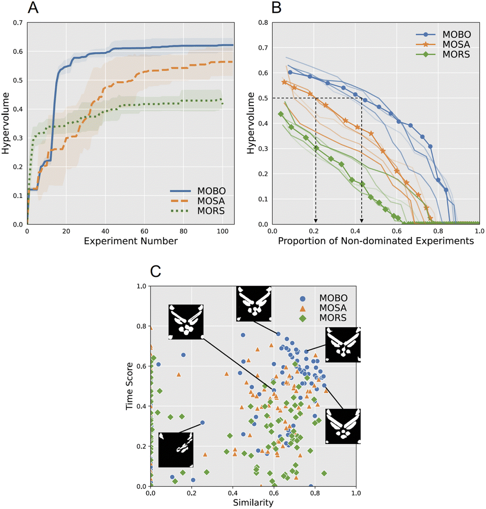Fig. 8 (A) Performance comparison among the three algorithms in the Air Force logo printing campaigns. Each bold curve shows the mean averaged across 5 campaigns per algorithm type, with ∼100 experiments in each campaign. The shaded band shows one standard deviation from the mean. (B) Quality of Pareto optimal solutions from the ten campaigns in panel A. The blue curve with dots, the orange curve with asterisks, and the green curve with diamonds represent results from the first MOBO, MOSA, and MORS campaigns, respectively. Each point on a curve represents the proportion of designs that achieved the hypervolume level on the y-axis or higher. For example, the left-most blue dot shows that MOBO achieves the hypervolume of 0.602 with 8.6% of the non-dominated experiments. The second blue dot includes more experiments that are not dominated by the other experiments other than the first set of non-dominated experiments. These additional experiments achieve the hypervolume of 0.585. The positions (values) of the other blue dots and yellow asterisks were obtained in the same way. See Algorithm 1 for further technical details. Results for the other four campaigns per algorithm type are shown in blue, orange, and green curves without dots, asterisks, and diamonds for visual clarity. The black arrows show the performance comparison between MOBO and MOSA for a given hypervolume of 0.5; more than 40% of the design samples achieve the hypervolume of 0.5 or higher in MOBO whereas it was only about 20% of the design samples in MOSA. (C) The empirical Pareto fronts from three selected campaigns, one per algorithm type. Shown in the insets are five sample prints for MOBO. Larger, high-resolution images overlaid on the target region are shown in Fig. 5.

The informativeness, or information gain, of an algorithm's hypervolume improvement depends on the efficiency of sampling the Pareto front. The algorithm should concentrate its exploration of the input space on the regions that are most promising for finding new combinations of the two objectives that dominate (have higher objective scores than) previous experiments. Fig. 8C shows both objective scores for each of the three algorithms over a single campaign. Note that the distribution of objective scores differs greatly across algorithms. For MORS, the distribution is almost bimodal along the similarity objective, with hypervolume values below 0.4 (many stacked at 0) or widely distributed above this value. MOSA exhibits a similar distribution, although as a group it contains higher time scores. MOBO, in contrast, has a number of points in the upper right that together define a Pareto front, suggesting that its search is more efficient and informative. We examine each of these qualities in turn.

We quantified algorithm efficiency by measuring the quality of its solutions in a campaign. In practice, we want to find as many optimal and nearby sub-optimal scores (which can be potentially as good as those in the estimated Pareto front) as possible to be confident in the algorithm's solution. The greater the concentration of points in this region, the more well-defined the front. The analysis can be conceptualized as layers of an onion. Imagine an onion centered at the origin (0, 0) of the solution space in Fig. 8C. Because the similarity and time scores are scaled between 0 and 1, our view in the graph can be thought of as one quarter of the onion. The Pareto front obtained at the end of a campaign (which we will call the ‘first’ Pareto front) forms an arc connecting the observations that constitute the largest possible radius; this arc of points corresponds to the outermost layer of the onion. These points, which are not dominated (i.e., not exceeded) by any others, are then counted and their combined hypervolume is computed. Next, these design points are removed (the first and outermost layer of the onion is peeled off) and those remaining define a second Pareto front, which corresponds to the new, outermost layer of the onion. Again, the number of points that form the front is counted and its hypervolume is computed. This peeling-off process repeats until all points are assessed and counted, the formal steps of which are described in Algorithm 1.

To generate the Pareto front plots in Fig. 8B for the Air Force logo printing campaigns and in Fig. 9B for the 2D Test Specimen printing campaigns, discussed in the next section, we used the “peeling-the-onion” strategy presented in Algorithm 1. Formally speaking, the algorithm comprises five steps: (1) we start with the set of objective scores of all design samples obtained from a campaign; (2) find the set of non-dominated designs ; (3) count the number of elements in the set and compute its hypervolume ; (4) define a new set by excluding from (i.e., ); (5) we repeat this procedure with , , , and for k = 1, 2, … until becomes empty . After the procedure described above, we compute the cumulative number of design samples for each of the k-th Pareto front. For k = 1, it is simply the number of design samples in the first Pareto front . For k = l, it is the sum of the number of design samples removed at steps k = 1, …, l. Finally, we plot (but as proportions with respect to the total number of experiments conducted) on the x-axis against on the y-axis to generate Fig. 8B, and similarly, Fig. 9B.

Fig. 9 (A) Performance comparison among the three multi-objective optimization algorithms in the 2-D test specimen (2DTS) printing campaigns. (B) Quality of Pareto optimal solutions from the ten campaigns in panel A. (C) The empirical Pareto fronts from a selected campaign per each algorithm type. Shown in the insets are four sample prints for MOBO. Larger, high-resolution images overlaid on the target region are shown in Fig. 5. For an interpretation of the data in each plot, see the discussion of the logo results in the caption of Fig. 8.

The results of this analysis are shown in Fig. 8B, with the curves describing the results for the five campaigns. The thickest lines denote the first campaign. To the extent there are non-dominant points, there will be more than one Pareto front. Together they form a function, the slope of which describes the compactness, or distribution, of fronts. Shallow slopes describe fronts that are closely packed, whereas steep slopes indicate fronts that have greater separation from one another. We focus on MOBO and MOSA because they are the most competitive. The number of dots along each function specifies the number of hypervolumes (fronts) computed, which is similar for both algorithms (MOBO: 14, MOSA: 13). What differs between them is their distributions. Although both functions start at a similar hypervolume (e.g., 0.602 vs. 0.563 for MOBO and MOSA, respectively), their trajectories differ. The slope of the MOBO function is shallower, with adjacent hypervolumes not differing much from each other. The slope becomes steep only when hypervolumes are low; note that there are very few hypervolumes below 0.3, indicating that MOBO, on the whole, rarely chose designs that yielded a low hypervolume. In contrast, successive fronts for MOSA drop more rapidly in hypervolume, resulting in a function with a steeper slope. Further, the relatively even spacing of the fronts along the function reveals that MOSA sampled regions of the design space that yielded low hypervolumes just as much as it sampled regions that led to medium and high hypervolumes. This difference between the two algorithms is replicated across campaigns, as the separation of the orange and blue functions shows.

The above efficiency analysis describes the thoroughness with which the algorithms trade off the two objectives to define the Pareto front. Their differences can be understood further by comparing the algorithms for a given hypervolume. The black arrows in Fig. 8B show the comparison between MOBO and MOSA with the hypervolume of 0.5 as a criterion; more than 40% of the design samples achieve the hypervolume of 0.5 or greater with MOBO whereas only about 20% reached this level with MOSA. Similarly, large differences are found for other hypervolumes. What these observations mean is that MOBO searches the design space selectively and intelligently, probing potentially promising new regions experiment after experiment based on what it has learned, which leads to an efficient mapping of the Pareto front in under 13 hours in the AM-ARES system.

A desirable byproduct of MOBO's efficiency in the current context is that, with a large enough campaign, the Pareto front describing the trade-off between the two objectives can be drawn. Returning to Fig. 8C, the insets in the figure are printed logos from five experiments that show differences in quality (similarity) and print time, providing additional evidence that the algorithm works as intended. The trade-off is visible in the three right images. Moving from the top to the bottom, one can see that faster print speed trades off with logo quality (notice the difference in the fullness and definition of the wings). MOBO identifies the relation between input parameters and objective scores that generate the front. This information puts researchers in a position to formalize the association, thereby creating a quantitative description to use for achieving one's printing objectives.

4.3 2D test specimen (2DTS) printing campaigns

Fig. 9 contains the results from a second study that we conducted to assess the generality of the results from the Air Force logo printing campaigns discussed in the preceding section. The shape was customized to be challenging to print. The outcome is qualitatively the same. MOBO's greater efficiency leads to a larger final hypervolume and a more well-defined Pareto front. The results differ from the previous study in that the difference between MOBO and MOSA is smaller. This could be attributed to an expected increased difficulty with respect to similarity scoring and an unexpected decreased difficulty with respect to print time scoring as compared to the Air Force logo. Indeed, there seemed to be an anisotropic bimodality in the Air Force logo case that is much less pronounced for the 2DTS shape due to shifting of the higher-performing data points along the similarity score axis.

5 Discussion

The overarching goal of our research is to integrate artificial intelligence and machine learning in order to increase the capabilities of autonomous research systems (ARES) in materials development and discovery. The particular purpose of the present study was to explore the application of Bayesian optimization to simultaneously optimize multiple objectives of an AM process in a complex and high-dimensional parameter space. AM-ARES, assisted by the multi-objective Bayesian optimization (MOBO) algorithm, succeeded in identifying a set of six parameter values that optimize two printing objectives (similarity, time score) in less than 100 experiments. MOBO's performance exceeded that of two comparison algorithms, and the generality and robustness of MOBO were demonstrated in repeated multiple print campaigns of two different test specimens.

This work, while highly encouraging, explores only a small fraction of the possible applications of AI in the field of AM. Although our experimental platform employs a volumetric syringe extrusion system, there are many other types of AM systems that fall into the same materials extrusion category, such as fused deposition modeling (FDM). There are numerous other categories of AM technologies that stand to benefit from closed-loop autonomous experimentation including powder-bed fusion, material jetting, and vat polymerization. We have also limited our scope to only exploring an underlying component of extrusion-type 3D printing, i.e., a single layer, which reduces the number of potential parameters available for optimization. We chose this crawl-before-you-walk approach in order to gain important foundational insight into the implementation of BO in real-world additive manufacturing systems. Indeed, for most types of 3D printing, a complete 3D component is comprised of hundreds, if not thousands, of individual layers built one upon the other. Hence, the overall quality of a 3D component is heavily reliant upon the quality of each individual layer. In opting to analyze single layer prints, we have also made it possible to employ a somewhat simple feedback mechanism in the form of single images. Not only does this lower the barrier to access for others to pursue this work, but it also enables low-cost duplication by students, hobbyists, etc. Who may not have access to expensive characterization equipment. Certainly, more comprehensive and sophisticated studies can be carried out by incorporating expensive equipment and more advanced analysis software, and this has been demonstrated.⁵

Another topic to pursue is transfer learning. Can an artificial agent like MOBO, which has learned one task, transfer the acquired knowledge and strategies to a different task in order to learn faster? For example, a 2D printer that learned to optimize print conditions for the Air Force logo would subsequently learn to print the 2DTS more efficiently, i.e., in fewer experiments. One way to answer this question in the current study without testing it explicitly is to assess whether optimized inputs are similar across the two objects. If they are, it is reasonable to infer that such transfer of learning would be found. The two objectives, similarity score and time score, should be largely independent of the object being printed. Optimal settings are therefore likely to be similar across objects except in cases where MOBO is sensitive to objet-specific characteristics.

Our analysis compared the optimality of the input parameters across their ranges for the two objects. We first created a composite measure of optimality, defined as the product of the similarity score and time score in an experiment. By determining the value of each parameter across all 105 experiments and 5 campaigns (525 observations), one can identify parameter regions that led to low and high optimality values. To the extent that printer inputs for the Air Force logo and 2DTS specimens were optimized similarly, these regions should be similar. To visualize these regions and compare them across print objects, we created contour plots of optimality values for nine selected pairings of parameters that we felt would be most informative to evaluate similarity. Fig. 10 contains contour plots for line width and print speed (see the supplement for the others). Although not identical, the graphs are quite similar. The lower part of the diagonal in both graphs contains very low scores. Only when line width exceeds 0.2 and print speed exceeds 1.0 (roughly the upper part of the diagonal) is performance enhanced. Increasing both inputs together tends to lead to a more optimal setting. Although this association is not surprising, a benefit of MOBO, as demonstrated above, is that it efficiently defines this relationship, and those among all parameters, across the ranges of the inputs given the equipment in use (filament, extruder, etc).

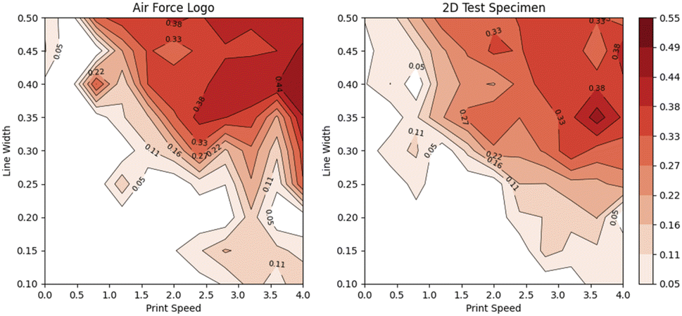Fig. 10 Contour plots of the composite measure (the product of similarity score and time score) for the combination of line width and print speed. The calculated difference between the respective contours is 0.62.

We quantified the similarity of the optimal parameterizations as the normalized absolute mean difference between the matrices of values that make up the contour plots. The mean difference across the nine plots is 0.089 (range: 0.062–0.125), indicating substantial similarity for a subset of inputs. This outcome leads us to expect that if the optimal settings were swapped between objects, the resulting experiments would yield hypervolumes that are on or close to their respective Pareto fronts. Plans are underway to explore this idea and cross-object parameter comparison more formally.

The present results, taken together, lay the groundwork for a variety of more ambitious studies. Our future plans include an extremely low-cost FDM version of AM-ARES that can be easily deployed in schools and other academic institutions to promote accessibility to state-of-the-art research tools while simultaneously harnessing the power of crowd-sourcing. Our hopes are that this will spur innovation and accelerate the development of AI for AM. To directly build upon the work demonstrated here, we will continue to explore the boundaries of MOBO in AM. How many real-world input parameters can BO effectively control? How many simultaneous objectives?

Turning the discussion to the technical aspects of the MOBO algorithm, despite the impressive progress in Bayesian optimization in particular, and kernel-based non-parametric optimization in general, there is still a central problem that needs to be addressed for virtually all applications of such machine learning methods. This is the problem of deciding which one among a set of applicable models (e.g., Gaussian process kernels) to use given an optimization task at hand and how to set its hyperparameters (e.g., length scale and variance parameters of a chosen kernel model). It is well known that the hyperparameters and other structural properties of a machine learning algorithm can significantly impact its performance and efficiency. It is a challenging combinatorial search problem that is generally intractable to solve manually via hand-tuning. The fully automated method for finding a solution is referred to as hyperparameter optimization or more broadly automated machine learning (AutoML).^50–53 At its core, an AutoML approach solves the problem by automatically (without human intervention) identifying the best model and fitting its hyperparameters. This is done dynamically and efficiently on a given dataset. In the present work, we applied a relatively simple Bayesian approach for adaptively optimizing the hyperparameters of our MOBO algorithm, as done.²⁵ Recently, more advanced and computationally intensive AutoML approaches have been introduced to address the problem.^54–57 Future work will focus on applying these techniques to multi-objective Bayesian optimization in AM.

The MOBO algorithm can also be extended to handle more complex scenarios in practice. That is, Bayesian optimization, by construct, assumes that the “black-box” objective function to be optimized is defined over a set of continuous experimental parameters. Many real-world problems, however, involve not only continuous variables but also discrete variables. For example, in extrusion-based 3D printing, the infill pattern for an object can be selected from among a diverse assortment of distinct options (e.g. solid, hexagonal, cubic, etc.). Optimizing an objective function over a mixture of discrete and continuous parameters is nontrivial both conceptually and computationally. Further, and related, it would be computationally prohibitive to search for an optimal solution due to the combinatorial explosion of a discrete search space. Despite these challenges, computer scientists have recently developed some promising solutions.^27,58 In essence, the basic idea of these approaches is to define continuous “proxy” variables as stand-ins for discrete variables so that the whole problem is turned into a standard Bayesian optimization problem.

6 Conclusion

Our successful demonstration of a multi-objective Bayesian optimization planner for additive manufacturing pushes the boundaries of integrating machine learning with AI Science for materials development and discovery. Instead of one-at-a-time, sequential optimization of AM printing parameters, which is slow and can lead to sub-optimal printing processes, MOBO shows that multiple parameters can be simultaneously optimized in a complex printing parameter space. This work points the way towards more complex campaigns of experiments with more objectives and more controlled input parameters that will ultimately afford researchers the ability to tackle research problems with high degrees of complexity. Indeed, our work shows the value of AM-ARES as a platform to develop and prove AI and autonomy planning approaches for optimal experimental design and scientific discovery.^59–61

Data availability

Data and processing scripts for this paper, including experimental and simulated data, along with data plots are available at Center for Open Science OSF at https://osf.io/3bpjm/.

Author contributions

J. Myung and M. Pitt: project administration, conceptualization, supervision, writing – original draft. B. Maruyama: conceptualization, review and editing. J. Deneault: experimental set-up and design, data curation, writing – materials and methods. J. Chang: methodology, algorithm implementation. I. Kang: simulation, data analysis.

Conflicts of interest

There are no conflicts to declare.

Acknowledgements

The work was supported by the Air Force Office of Scientific Research (AFOSR) grant FA9550-21-1-0176 to MAP and JIM.

Notes and references

1. A. Atkinson and A. Donev, Optimum Experimental Designs, Oxford University Press, 1992.
2. B. Settles, Synth. Lect. Artif. Intell. Mach. Learn., 2012, 6, 1–114.
3. P. Nikolaev, D. Hooper, F. Terrones and B. Maruyama, ACS Nano, 2014, 8, 10212–10222.
4. P. Nikolaev, D. Hooper, F. Webber, R. Rao, K. Decker, M. Krein, J. Poleski, R. Barto and B. Maruyama, npj Comput. Mater., 2016, 2, 16031.
5. A. E. Gongora, B. Xu, W. Perry, C. Okoye, P. Riley, K. G. Reyes, E. F. Morgan and K. A. Brown, Sci. Adv., 2020, 6, 1–7.
6. E. L. Snapp, B. Verdier, A. E. Gongora, S. Silverman, A. D. Adesiji, E. F. Morgan, T. J. Lawton, E. Whiting and K. A. Brown, Nat. Commun., 2024, 15(4290), 1–9.
7. E. Stach, B. DeCost, A. G. Kusne, J. Hattrick-Simpers, K. A. Brown, K. G. Reyes, J. Schrier and B. Maruyama, Matter, 2021, 4, 2702–2726.
8. J. Chang, P. Nikolaev, J. Carpena-Nunez, R. Rao, K. Decker, A. E. Islam, J. Kim, M. A. Pitt, J. I. Myung and B. Maruyama, Sci. Rep., 2020, 10, 1–9.
9. R. Deneault, J. Chang, J. I. Myung, D. Hooper, A. Armstrong, M. A. Pitt and B. Maruyama, Mater. Sci. Res., 2021, 46, 566–575.
10. D. R. Cavagnaro, J. I. Myung, M. A. Pitt and J. V. Kujala, Neural Comput., 2010, 22, 887–905.
11. J. I. Myung, D. R. Cavagnaro and M. A. Pitt, J. Math. Psychol., 2013, 57, 53–67.
12. J. Chang, J. Kim, B.-T. Zhang, M. A. Pitt and J. I. Myung, Cognit. Psychol., 2021, 125, 1–18.
13. J. Bhattacharjya, S. Tripathi, A. Taylor, M. Taylor and D. Walters, Working Conference on Virtual Enterprises, 2014, pp. 365–372.
14. J. C. de Oliveira Matias, C. M. O. Pimentel, J. C. G. dos Reis, J. M. C. M. das Dores and G. Santos, Quality Innovation and Sustainability: 3rd ICQIS, Aveiro University, Portugal, May 3-4, 2022, Springer Nature, 2023.
15. Y. Wu, J. Fang, C. Wu, C. Li, G. Sun and Q. Li, Int. J. Mech. Sci., 2023, 108102.
16. T. Erps, M. Foshey, M. K. Luković, W. Shou, H. H. Goetzke, H. Dietsch, K. Stoll, B. von Vacano and W. Matusik, Sci. Adv., 2021, 7, eabf7435.
17. M. Jani, Cura Settings Decoded – An Ultimaker Cura Tutorial, 2022, https://all3dp.com/1/cura-tutorial-software-slicer-cura-3d/.
18. M. Dwamena, Cura Settings Ultimate Guide – Settings Explained & How to Use, https://3dprinterly.com/cura-settings-ultimate-guide-settings-explained-how-to-use/.
19. AmeraLabs, The Complete Resin 3D Printing Settings Guide for Beginners, 2022, https://ameralabs.com/blog/the-complete-resin-3d-printing-settings-guide-for-beginners/.
20. Subcommittee on the Materials Genome Initiative Committee on Technology, A Report on Material Genome Initiative Strategic Plan, 2021, https://www.mgi.gov/sites/default/files/documents/MGI-2021-Strategic-Plan.pdf.
21. Y. Collette and P. Siarry, Multiobjective Optimization, Springer, 2003.
22. K. Swersky, J. Snoek and R. P. Adams, Adv. Neural Inf. Process. Syst., 2017, 26, 2004–2012.
23. A. Ozkis and A. Babalik, Inf. Sci., 2017, 402, 124–148.
24. S. Daulton, M. Balandat and E. Bakshy, Adv. Neural Inf. Process. Syst., 2020, 9851–9864.
25. S. Daulton, M. Balandat and E. Bakshy, Adv. Neural Inf. Process. Syst., 2021, 2187–2200.
26. I. Couckuyt, D. Deschrijver and T. Dhaene, J. Global Optim., 2014, 60, 575–594.
27. S. Daulton, X. Wan, D. Eriksson, M. Balandat, M. A. Osborne and E. Bakshy, Advances in Neural Information Processing Systems, 2022.
28. E. Zitzler, L. Thiele, M. Laumanns, C. M. Fonseca and V. G. da Fonseca, IEEE Trans. Evol. Comput., 2003, 7, 117–132.
29. J. Mockus, J. Global Optim., 1994, 4, 347–365.
30. J. Mockus, Bayesian Approach to Global Optimization: Theory and Applications, Kluwer, 1989.
31. D. R. Jones, M. Schonlau and W. J. Welch, J. Global Optim., 1998, 13, 455–495.
32. E. Brochu, V. M. Cora and N. De Freitas, arXiv, 2010, preprint, arXiv:1012.2599, pp. 1–49,  DOI:10.48550/arXiv.1012.2599.
33. B. Shahriari, K. Swersky, Z. Wang, R. P. Adams and A. de Freitas, Proc. IEEE, 2016, 104, 148–175.
34. P. I. Frazier, arXiv, 2018, preprint, arXiv:1807.02811v1, pp. 1–21,  DOI:10.48550/arXiv.1807.02811.
35. S. Greenhill, S. Rana, S. Gupta, P. Vellanki and S. Venkatesh, IEEE Access, 2020, 8, 13937–13948.
36. T. Pourmohamad and H. K. H. Lee, Bayesian optimization with application to computer experiments, Springer, 2021.
37. C. E. Rasmussen and C. K. I. Williams, Gaussian Processes for Machine Learning, MIT Press, Cambridge, MA, 2006.
38. A. M. Gopakumar, P. V. Balachandran, D. Xue, J. E. Gubernatis and T. Lookman, Sci. Rep., 2018, 8, 1–12.
39. B. P. MacLeod, F. G. L. Parlane, C. C. Rupnow, K. E. Dettelbach, M. S. Elliott and C. P. Berlinguette, Nat. Commun., 2022, 13(995), 1–10.
40. J. A. Garrido-Torres, S. H. Lau, P. Anchuri, J. M. Stevens, J. E. Tabora, J. Li, A. Borovika, R. P. Adams and A. G. Doyle, J. Am. Chem. Soc., 2022, 144, 19999–20007.
41. T. Chepiga, P. Zhilyaev, A. Ryabov, A. P. Simonov, O. N. Dubinin, D. G. Firsov, Y. O. Kuzminova and S. A. Evlashin, Materials, 2023, 16(1050), 1–11.
42. E. Inman, H. Noori, A. Deep and S. Ramesh, Prog. Addit. Manuf., 2024, 1–11.
43. E. S. Chen, A. Ahmadianshalchi, S. S. Sparks, C. Chen, A. Deshwal, J. R. Doppa and K. Qiu, Adv. Mater. Technol., 2024, 1–11.
44. B. V. Ultimaker, Ultimaker, 2023, https://ultimaker.com/.
45. S. Kirkpatrick, C. Gelatt and M. Vecchi, Science, 1983, 220, 671–680.
46. G. P. McCormick, Math. Program., 1976, 10, 147–175.
47. M. Jamil and X.-S. Yang, Int. J. Math. Model. Numer. Optim., 2013, 4, 150–194.
48. F. H. Branin and S. K. Hoo, Numerical Methods of Nonlinear Optimization, London, 1972.
49. C. Currin, T. Mitchell, M. Morris and D. Ylvisaker, A Bayesian approach to the design and analysis of computer experiments, Oak Ridge National Laboratory Technical Report 6498, 1988.
50. M. Feurer, A. Klein, K. Eggensperger, J. Springenberg, M. Blum and F. Hutter, in Advances in Neural Information Processing Systems 28, ed. C. Cortes, N. D. Lawrence, D. D. Lee, M. Sugiyama and R. Garnett, Curran Associates, Inc., 2015, pp. 2962–2970.
51. H. Rakotoarison, M. Schoenauer and M. Sebag, Proceedings of the Twenty-Eighth International Joint Conference on Artificial Intelligence (IJCAI), 2019, pp. 3296–3303.
52. F. Hutter, L. Kotthoff and J. Vanschoren, Automated Machine Learning, arXiv, preprint, arXiv:1810.13306v5, Springer, 2019,  DOI:10.48550/arXiv.1810.13306.
53. Q. Yao, M. Wang, Y. Chen, W. Dai, Y.-F. Li, W.-W. Tu, Q. Yang and Y. Yu, preprint, ArXiv:1810.133064v4, 2019, 1–20.
54. D. Duvenaud, J. R. Lloyd, R. Grosse, J. B. Tenenbaum and Z. Gjajramani, Proceedings of the 30th International Conference on Machine Learning, Atlanta, Georgia, 2013, pp. 1166–1174.
55. G. Malkomes, C. Schaff and R. Garnett, Advances in Neural Information Processing Systems, 2016.
56. G. Malkomes and R. Garnett, Advances in Neural Information Processing Systems, 2018.
57. J. Kirschner, M. Mutny, N. Hiller, R. Ischebeck and A. Krause, Proc. Mach. Learn. Res., 2019, 97, 3429–3438.
58. B. Ru, A. S. Alvi, V. Nguyen, M. A. Osborne and S. J. Roberts, Proceedings of the Thirty-seventh International Conference on Machine Learning (ICML), 2020.
59. W. B. Powell and I. O. Ryzhov, Optimal Learning, Wiley, 2012.
60. S. Chen, K. G. Reyes, M. K. Gupta, M. C. McAlpine and W. B. Powell, SIAM/ASA J. Uncertain. Quantification, 2015, 3, 320–345.
61. H. Kitano, npj Syst. Biol. Appl., 2021, 7, 1–12.

---

Footnotes

† The smoothness parameter value of ν = 2.5 was chosen manually after trying several preliminary campaigns of printing experiments, whereas the length-scale parameter l was optimized online jointly with the surrogate model itself using Python's BoTorch package.

‡ Our implementation of MOSA used an initial temperature T = 100 and cooling factor λ = 0.9 for all experiments shown.

§ The two objective functions for the easy case in Fig. 6A are the McCormick function⁴⁶ and the Matyas function,⁴⁷ both with a single global optimum. The two objective functions for the challenging case in Fig. 6B are the Branin function⁴⁸ with three global optima and the Currin function with a single global optimum at the boundary.⁴⁹

---