
 Open Access Article
 This Open Access Article is licensed under a
 Creative Commons Attribution 3.0 Unported Licence
Hydrodynamic slip in nanoconfined flows: a review of experimental, computational, and theoretical progress
Abdul Aziz
Shuvo
 a,
Luis E.
Paniagua-Guerra
a,
Juseok
Choi
b,
Seong H.
Kim
bcd and
Bladimir
Ramos-Alvarado
*a
a,
Luis E.
Paniagua-Guerra
a,
Juseok
Choi
b,
Seong H.
Kim
bcd and
Bladimir
Ramos-Alvarado
*a
aDepartment of Mechanical Engineering, The Pennsylvania State University, University Park, Pennsylvania 16802, USA. E-mail: bzr52@psu.edu
bDepartment of Chemical Engineering, The Pennsylvania State University, University Park, Pennsylvania 16802, USA
cDepartment of Material Science and Engineering, The Pennsylvania State University, University Park, Pennsylvania 16802, USA
dDepartment of Chemistry, The Pennsylvania State University, University Park, Pennsylvania 16802, USA
First published on 12th November 2024
Abstract
Nanofluidics has made significant impacts and advancements in various fields, including ultrafiltration, water desalination, biomedical applications, and energy conversion. These advancements are driven by the distinct behavior of fluids at the nanoscale, where the solid-fluid interaction characteristic lengthscale is in the same order of magnitude as the flow conduits. A key challenge in nanofluidics is understanding hydrodynamic slip, a phenomenon in which fluids flow past solid boundaries with a non-zero surface velocity, deviating from the classical no-slip boundary condition. This review consolidates experimental, computational, and theoretical efforts to elucidate the mechanisms behind hydrodynamic slip in nanoconfined flows. Key experimental methods, such as the surface force apparatus, atomic force microscopy, and micro-particle image velocimetry are evaluated alongside emerging techniques like suspended microchannel resonators, dynamic quartz crystal microbalance, and hybrid graphene/silica nanochannels, which have advanced hydrodynamic slip characterization at the nanoscale. In addition to direct slip measurement techniques, methods like sum frequency generation spectroscopy, X-ray reflectometry, and ellipsometry are discussed for their roles in probing solid-liquid interfacial interactions, shedding light on the origins of hydrodynamic slip. The review also highlights the contributions of molecular dynamics simulations, including both non-equilibrium (NEMD) and equilibrium (EMD) approaches, in modeling interfacial phenomena and slip behavior. Additionally, it explores the influence of factors such as surface wettability, shear rate, and confinement on slip, emphasizing the interaction between liquid structuring and solid–liquid interactions. Advancements made so far have uncovered more complexities in nanoconfined flows which have not been considered in the past, inviting more investigation to fully understand and control fluid behavior at the molecular level.
 Abdul Aziz Shuvo | Abdul Aziz Shuvo is a Ph.D. candidate in Mechanical Engineering at The Pennsylvania State University and an Assistant Professor (on leave) at Bangladesh University of Engineering and Technology (BUET). His research focuses on interfacial phenomena, electronics cooling, turbulence, and multiscale modeling. He earned both his Bachelor's (2019) and Master's (2022) degrees in Mechanical Engineering from BUET. Before his appointment at BUET, he briefly served as a lecturer at Ahsanullah University of Science and Technology, Dhaka (AUST). Later, he was promoted to Assistant Professor at BUET in 2022. |
 Luis E. Paniagua-Guerra | Dr. Luis E. Paniagua-Guerra is a Postdoctoral Scholar in the Mechanical Engineering Department at The Pennsylvania State University. He received his PhD and master's degree in mechanical engineering from The Pennsylvania State University and a bachelor's in mechanical engineering from the University of Guanajuato in Mexico. His major interests include the fundamental study of nanoscale thermal, hydraulic, and mechanical properties via atomistic level modeling, the study of solid–liquid interfacial phenomena, and the thermal characterization of liquid cooling solutions for electronics. |
 Juseok Choi | Juseok Choi is a Ph.D. candidate in the Department of Chemical Engineering at Pennsylvania State University, under the supervision of Prof. Seong H. Kim. He has studied the mesoscale structure of cellulose microfibrils in plants using sum-frequency generation (SFG) vibrational spectroscopy, with support from the Center for Lignocellulose Structure and Formation (CLSF). His current research focuses on the effect of the interfacial water structure at the solid–liquid interface on hydrodynamic slip behavior through experimental approaches. |
 Seong H. Kim | Prof. Seong H. Kim joined the faculty of Chemical Engineering at Penn State in 2001 after completing a Ph.D. in Chemistry at Northwestern University and conducting post-doctoral research at the University of California, Berkeley. He is currently a Distinguished Professor of Chemical Engineering and has courtesy appointments with the Department of Chemistry and the Department of Materials Science and Engineering at Penn State. Dr Kim's research interests lie in surface science and materials characterization. He has published more than 360 papers, and the h-index of his published work is 71. He recently finished writing a textbook on “Surface and Interface Analysis – Principles and Applications”, which is currently under production through Wiley and will come out in March 2025. |
 Bladimir Ramos-Alvarado | Dr. Bladimir Ramos-Alvarado is an Associate Professor of Mechanical Engineering and the principal investigator of the Interfacial Phenomena Lab (IPHEL) at the Pennsylvania State University (Penn State), he is a member of the Materials Computation Center at Penn State, and an Associate of the Institute for Computational and Data Sciences (ICDS) at Penn State. He also serves as a Subject Matter Editor for Applied Thermal Engineering (Elsevier). Dr. Ramos obtained a Bachelor's and a Master's degree, both in Mechanical Engineering, from the University of Guanajuato, Mexico, in 2009 and 2011, respectively. Later on, he continued his education at the Georgia Institute of Technology (Georgia Tech) where he obtained a PhD and a Master's degree in Mechanical Engineering in 2016. After brief Postdoctoral and Instructor appointments at Georgia Tech, Dr. Ramos joined the Department of Mechanical Engineering at Penn State University as an Assistant Professor in May 2017. |
1 Introduction
Investigations on nanoconfined fluids date to the first half of the last century. Following early investigations of fluid transport in nanoconfinements,1 the study of fluid flow at the nanoscale emerged as a new field of science called nanofluidics, a term coined in the 1990s.2,3 Furthermore, the integration of nanofabrication with nanofluidic technology offers potential breakthroughs in the manipulation and control of fluids at the molecular level, which could revolutionize our approach to a variety of scientific and industrial challenges. This surge in interest is driven by the capability of nanofluidic devices to operate with high efficiency and sensitivity due to their minute scale and the unique properties of fluids confined to such small dimensions.The application of nanofluidic devices could impact promising technologies, including biomedical applications, ultrafiltration and desalination processes, and ionic transport for energy conversion. In the biomedical field, nanofluidics may reduce the amount of genomic material and time for analysis of DNA.4–6 Nanochannel devices have therapeutic applications on high-precision drug delivery systems;7–10 while, nanoengineered fluidic devices enable low-cost cell analysis and disease diagnostics.11,12 Similarly, the integration of nanoconduits in lab-on-a-chip systems allows for single-cell analysis, increasing the reliability of portable point-of-care medical diagnostic systems.13,14 Beyond biomedical applications, nanoconfined fluid flows offer precise manipulation of ionic concentrations and enhance electrochemical-mechanical energy conversion in batteries.15 Such technologies also facilitate groundbreaking electrical energy production from salinity gradients.16,17 Furthermore, the active control of ion charge concentration in nanoflows is applied to the development of fluid-based devices analogous to micro-electronics, such as nanofluidic transistors18–20 and diodes.21–24 Another main research venue of nanofluidics takes advantage of the filtration capabilities of nanotubes and nanopores.25 Capillary devices with molecular-scale precision are used in ultrafiltration,26,27 while nanometer-scale porous membranes are promising alternatives for seawater desalination.28–32 In addition to the highly specialized applications discussed so far, the behavior of thin, confined fluids is essential in numerous industrial operations, mainly involving lubrication,33 nanoencapsulation,34 and nanofabrication.35 Electrospinning technologies leverage the interaction between electrostatic forces and working fluids at the spinneret nozzle to create innovative nanofabrication methods to produce hollow, core–shell, and multichannel nanofibers, which are crucial for high-performance materials used in catalysis, drug delivery, and energy storage.35
Along with the enhanced capabilities of nanofluidic devices comes a major increase in flow friction, which is an inevitable challenge. Fluid flow through minuscule confinements experiences a vast increase in flow resistance, per the classical hydrodynamics theory. The significance of friction in nanoconfined flows is attributed to the interfacial interactions as the surface-to-volume ratio increases at the nanoscale.36 However, due to the dominant effects of interfacial properties such as wettability and surface roughness, fluid flow in nanochannels can be tailored to overcome the hydraulic limitations imposed by high confinement levels. For instance, experimental investigations of flow in carbon nanotubes (CNT) have reported flow enhancements up to five times higher than expected from the conventional continuum theory.37–39 CNTs are atomically smooth surfaces with hydrophobic properties, a combination that hypothetically offers a reduced resistance to flow.
Nanoconfined flows have been described by classical fluid dynamics combined with atomistic modeling to account for interfacial interactions in nanochannels with diameters down to 1.4 nm.40 The applicability of the continuum approach facilitates the creation of a theoretical framework to model fluid flow. However, the boundary condition compatible with the continuum approach remains a challenge, i.e., accounting for and quantifying hydrodynamic slip.41–43 The earliest efforts to simulate flow through nanochannels resulted in flow velocities between 2 to 10 orders of magnitude higher than experimental measurements,44 indicating an overestimation of the hydrodynamic slip. Sophisticated simulations, considering complex wettability interactions41 and long averaged simulated times44 (∼100 μs) have been conducted in recent years, obtaining flow regimes comparable with the flow velocities reported in the experimental literature. However, a complete understanding of the mechanisms and significant parameters in nanoconfined flows is still needed.
In this literature review, the basics of hydrodynamics in nanoconfined flows are introduced in Section 2. A review of the experimental efforts aimed at explaining the different variables affecting hydrodynamic slip is presented in Section 3; the most relevant experimental techniques and the tendency towards higher resolution measurements are highlighted as well as the controversy regarding the effects of wettability and liquid structuring metrics on the hydrodynamic slip. Subsequently, a more comprehensive review of the modeling efforts for investigating the complex phenomena of nanoconfined flows is reported in Section 4. The different non-equilibrium and equilibrium methods for modeling fluid friction in nanochannels are revised and compared. Lastly, in Section 5 a more fundamental review of the underlying physics behind slip as well as the effects of wettability, shear rate, and confinement is presented. Fig. 1 illustrates a knowledge map outlining the contents of this review.
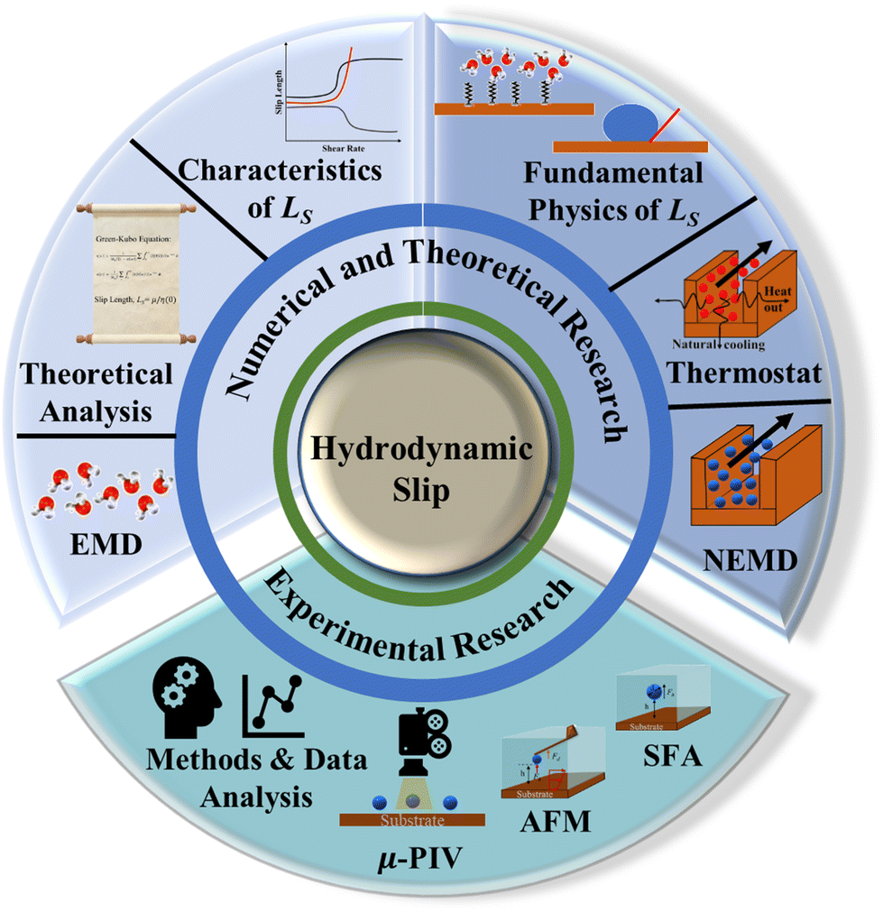 | ||
| Fig. 1 Knowledge map of the literature review on nanoscale hydrodynamic slip. | ||
2 Friction and hydrodynamic slippage in nanoconfined liquids
In macroscale fluid dynamics, the no-slip boundary condition has allowed experimental results to align with numerical and analytical models across various applications. Despite its widespread use, the no-slip boundary condition is phenomenological and not derived from fundamental physical principles.45 In Navier's early work,46 an alternative boundary condition that permits slippage has been suggested: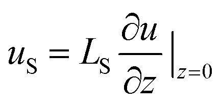 | (1) |
Conversely, the governing equations of continuum fluid mechanics have a solid theoretical foundation. In the continuum framework, Newton's second law is applied to infinitesimal volume elements large enough to preserve the bulk values of the thermophysical and transport properties of the fluid. After applying the Newtonian corollaries to the relation between stresses and deformations, the famous Navier–Stokes (NS) equations arise. However, these equations break down when the flow system is reduced to dimensions comparable to the molecular size due to the uncertainty of the continuum assumption.40
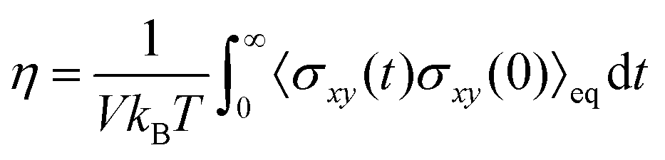
In the hydrodynamic regime where the NS equations are applicable, there is a distinct separation in length and time scales between bulk properties and surface effects.3 In bulk systems with particle quantities in the order of Avogadro's number, the molecular degrees of freedom can be described with only a few variables such as pressure, velocity field, temperature, etc., while the complexity of the transport phenomena is lumped into transport coefficients. Bocquet and Charlaix3 calculated the applicability range of the NS equations by determining the lower-scale limit for the concept of shear viscosity (η), which is represented by the Green–Kubo relation:
 | (2) |
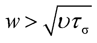 . For water τσ ∼ 10−12 s and υ = 10−6 m2 s−1 at 20 °C, which yield a limit of w ≈ 1 nm, proving the robustness of the NS equations. Thus, for water, confinement levels in the nanometer scale can be modeled using the classical governing equations of fluid mechanics. Notably, Thomas and McGaughey40 confirmed the bulk-like behavior of water flowing through CNT of diameters ∼1.4 nm.
3 Experimental investigations of hydrodynamic slip
Nanoconfined flowing liquids can be described by the equations of bulk hydrodynamics down to scales of approximately 1 nm (approximately three water molecular diameters). However, characterizing the boundary conditions for these flows remains challenging. The no-slip boundary condition has been successfully applied to macroscopic systems, where it remains phenomenologically valid. However, deviations from this condition arise at smaller scales where surface interactions dominate, casting doubt on its applicability at the nanoscale.Accurately measuring interfacial properties in nanofluidics is challenging due to the dynamic interactions at liquid–solid interfaces and spatial resolution limitations.3 Recently, these experimental challenges have been addressed significantly. For instance, the surface force apparatus (SFA) and atomic force microscopy (AFM) can directly access the hydrodynamic forces with high sensitivity in a controlled environment. Additionally, micro-particle image velocimetry (μ-PIV) enables the visualization of the velocity field in real time, which is critical for slip measurements. This Section will discuss these primary methodologies—SFA, AFM, and μ-PIV—and their recent developments in measuring LS in nanoconfinements. Moreover, Section 3.4 will explore emerging techniques for measuring LS using suspended microchannel resonators (SMRs), dynamic auartz crystal microbalance (QCM-D), and hybrid graphene/silica nanochannel techniques. Along with LS metrologies, surface characterization techniques, such as sum frequency generation (SFG) spectroscopy and X-ray reflectometry (XRR), will also be presented in Section 3.5. These techniques are useful in uncovering the origins of hydrodynamic slip behavior, particularly concerning the chemical interactions of interfacial water molecules.
3.1 Surface force apparatus (SFA)
The SFA measures the viscous force, Fh, between two surfaces submerged in a liquid with viscosity η, based on their separation distance h, and balanced by the cantilever restorative force, Fk,47 as shown in Fig. 2(a). This viscous force is detected using piezoelectric materials, and the gap between the surfaces is determined through interferometry. Employing SFA in conjunction with multiple beam interferometry enables measurements with sub-nanometer accuracy. The expression for Fh is provided in eqn (3) where va represents the relative approach velocity of the surfaces, r is the radius of the sphere immersed in the liquid, and f* is a correction factor that compensates for hydrodynamic slip. When f* = 1, eqn (3) corresponds to the NS solution in the lubrication approximation. For surfaces of comparable characteristics, Vinogradova48 derived the solution for f* as detailed in eqn (4).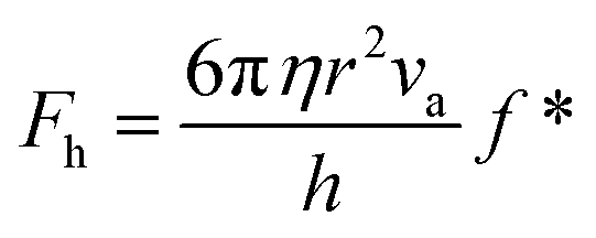 | (3) |
 | (4) |
 | ||
| Fig. 2 Schematic of the operational principles of (a) SFA, (b) AFM, and (c) μ-PIV. In (a) and (b), the radius of the spherical probe (r), surface separation distance (h), and probe approach velocity (va) are indicated as the parameters of the hydrodynamic drag force (Fh) and the restorative force of the cantilever (Fk), which are balanced for the hydrodynamic slip measurement. | ||
Chan and Horn49 investigated the drainage of three non-polar organic Newtonian liquid films between molecularly smooth mica surfaces using the SFA. Their results were in good agreement with the Reynolds theory of lubrication (no-slip boundary condition) for film thicknesses above 50 nm; however, for thinner films, an apparent enhancement of the liquid's viscosity was observed. Chan and Horn49 indicated that as the film thickness decreases, the surface effects are more significant and produce a “solid-like” ordering in the liquid layers near the wall, causing an increase in the liquid resistance to shear. A modification to the formerly static SFA apparatus is reported in Luengo et al.50 where a shear attachment was added to the original design, now allowing for dynamic rheological analyses. A series of transition regimes in the rheological behavior of polymer melts as well as a reduction of viscosity with film thickness were found using the modified SFA.
Baudry et al.51 used a similar version of the dynamic SFA to investigate the slippage of glycerol in contact with wetting and non-wetting surfaces. On a wetting cobalt surface, the no-slip boundary condition was observed; alternatively, when cobalt was coated with a thiol, the surface became non-wetting, and LS ≈ 65 glycerol molecular diameters was measured. The liquid confined between wetting surfaces showed a constant viscosity as the confinement was varied; in contrast, for non-wetting cobalt-thiol, a reduction in the liquid viscosity was observed as the separation between surfaces decreased.
High shear rates have been observed to trigger bubble nucleation, leading to increased slip. Zhu and Granick52 observed large LS with water and tetradecane on hydrophobic surfaces, noting that LS escalated unboundedly as shear rates increased in their experiments, reaching up to the micrometer range. Furthermore, Cottin-Bizonne et al.53 investigated the hydrodynamic boundary conditions of water and dodecane on both hydrophobic and hydrophilic surfaces, employing a dynamic SFA under shear rates up to 5 × 10³ s−1. They found that the viscosity of water remained consistent with its bulk value in confinements as narrow as 10 nm. On hydrophilic Pyrex surfaces, neither water nor dodecane exhibited hydrodynamic slip; however, on hydrophobic surfaces, both fluids showed slip with LS reaching approximately 20 nm.
The findings by Cottin-Bizonne et al.53 present notable contradictions to those of Zhu and Granick.52 Cottin-Bizonne et al.53 noted that the oscillation amplitude of pressure in their SFA experiments remained below the vapor pressure of the examined liquids, precluding cavitation, which might have been possible under the conditions used by Zhu and Granick.52 Furthermore, they hypothesized that discrepancies could arise from the contamination of surfaces by hydrophobic materials. Continuing this investigation, Cottin-Bizonne et al.54 also explored potential experimental inaccuracies affecting their results. They highlighted that even small miscalculations in measuring the separation distance between surfaces could significantly impact the calculated LS. Their further studies using water and water mixtures aimed to discern the impact of viscosity on different wettability surfaces, finding that surfaces with higher hydrophobicity exhibited greater LS, though not exceeding 20 nm.
3.2 Atomic force microscopy (AFM)
AFM, as described in Fig. 2(b), employs the same approach and equations eqn (3) and (4) as the SFA. However, AFM probes smaller areas, which are determined by the size of the spherical bead attached to the AFM probe.3 Craig et al.55 utilized an AFM setup to assess the drainage force in aqueous sucrose solutions between a spherical tip and a flat surface. They employed analytical models to determine variables such as LS from the measured force–distance curves. They observed that the LS varied with the fluid's viscosity and the rate at which the AFM cantilever approached (shear rate). At lower velocities, there was no slip, indicative of a “free system” behavior, whereas at higher velocities LS ≤ 20 nm were reported. A notable limitation of AFM in measuring viscous forces in nanoconfined liquids is its sensitivity to deflections in the AFM cantilever caused by viscous drag.56 To address this, Vinogradova et al.56 developed multiple models aimed at curbing or even eliminating the increase in viscous drag as the speed of the AFM cantilever escalated. Further, Vinogradova et al.57 engineered an AFM probe that reduced drag. Employing a data reduction method previously outlined by Vinogradova et al.,56 they successfully identified the no-slip boundary condition and measured an LS of 10 nm on hydrophobic surfaces.Using AFM, Bonaccurso et al.58 assessed the hydrodynamic force between hydrophilic mica and glass in the presence of aqueous solutions, measuring LS of 8–9 nm on these surfaces, irrespective of the AFM probe approach speed. The experiments were conducted at high shear rates (104 s−1), which accounted for the observed hydrodynamic slippage on the hydrophilic surfaces. Honig and Ducker59 explored the impact of rapidly approaching AFM probes on measuring viscous forces within sucrose solutions varying in viscosity. They observed no significant increase of LS exceeding zero, even at shear rates up to 2.5 × 10⁵ s−1, contrasting with the results from Bonaccurso et al.58 when examining similar systems. However, their findings were in line with those of Vinogradova et al.57 The discrepancies are thought to stem from the different methods used to measure the gap between the surface and the probe. Traditional AFM experiments calculate this distance using the combined displacement of the piezoelectric scanner movement and the cantilever deflection, while Honig and Ducker59 derived the separation distance through the intensity of scattered evanescent waves. Bhushan et al.60 investigated LS for different surface conditions using the AFM tapping mode. The authors reported LS values of 43 nm and 232 nm for hydrophobic and superhydrophobic surfaces, respectively. Maali et al.61 enhanced the design of commercially available AFM cantilevers by adapting them for improved acoustic excitation in liquid environments. They integrated an anti-reflective coated glass slide into the cantilever holder to reduce unwanted oscillation peaks. Subsequently, Maali et al.62 used this improved version of the AFM to measure the LS of water on graphitic-carbon surfaces at a value of 8 nm.
In AFM experiments, instrumental uncertainties such as offsets and improper calibrations result in significant errors in determining LS.54,63 Such errors originate from the necessity of independently providing accurate values for the liquid viscosity, spherical AFM probe radius, and AFM cantilever spring constant when calculating LS, as inaccuracies in these parameters can propagate and lead to incorrect slip estimations.54 For example, Bonaccurso et al.58 reported LS of approximately 8 nm for a hydrophilic substrate (mica–water interface), while Maali et al.64 and Zhang et al.65 reported values close to zero. To overcome these discrepancies, a new data analysis model was proposed, assuming that the diameter of the microsphere is much larger than the slip length.54,66,67
 | (5) |
3.3 Micro-particle image velocimetry (μ-PIV)
The μ-PIV method, as illustrated in Fig. 2(c), involves tracking particle movement within a liquid flow constrained to microscale dimensions. This technique focuses image velocimetry analysis on areas close to the surface to sample the velocity profile and observe interfacial phenomena. Although theoretically applicable to nanoscale conduits, μ-PIV faces significant challenges in accurately tracking particles that are only a fraction of the size of the nanochannels. Additionally, as the resolution of μ-PIV improves, the measurements become noisier due to increased Brownian motion affecting smaller tracer particles.3 Consequently, μ-PIV is typically employed in microchannels, with efforts concentrated on enhancing resolution near the surface to detect the presence of hydrodynamic slip. Tretheway and Meinhart45 utilized standard μ-PIV to investigate slip in hydrophilic and hydrophobic channels with a cross-section area Across-section = 30 × 300 μm2. They used fluorescent polystyrene spheres with a diameter of 300 nm as tracers in the sampled region measuring 25 μm × 100 μm. They reported LS = 1 μm for hydrophobic surfaces, while no-slip (LS = 0) for hydrophilic conditions. These findings exceeded theoretical predictions but aligned with the expected effects of wettability.Lumma et al.69 enhanced the precision of velocity profiling within a 100 μm wide microchannel by using the fluorescence correlation spectroscopy (FCS) method to cross-correlate the fluorescence signals of clearly identified tracer particles with a diameter of 40 nm. This approach distinguishes between flow and diffusion effects, revealing LS ranging from 0.2 to 1 μm. They recognized that their measurements of LS might be larger, influenced by interactions between the liquid and surface and the repulsive forces among the tracer colloids. In another investigation using conventional μ-PIV, Ou and Rothstein70 measured LS of 7.5 μm in micro-ridges with ultra-hydrophobic surfaces and a shear-free configuration. Their results also matched independent experiments using a pressure drop calculation of slip. Joseph and Tabeling71 refined the μ-PIV method significantly, achieving near-simulation accuracy. They used fluorescent beads ranging from 100 to 200 nm in diameter within a microchannel measuring 10 μm × 100 μm. To precisely ascertain the wall position, they tracked the location of tracer particles that adhered to the walls, reporting LS < 100 nm, with uncertainties comparable to the measured values.
3.4 Other techniques for direct slip measurement
In addition to the hydrodynamic slip characterization techniques described in Sections 3.1–3.3, there are methods to directly measure LS. Collis et al.72 first proposed LS measurements on individual gold nanoparticles immersed in water. They used suspended microchannel resonators (SMRs) introducing gold nanoparticles into “U-shaped” channels embedded in a cantilever. When a nanoparticle passes through the channel, it increases the inertial mass of the sensor. In the experiments, the flow at the particle's surface is closely related to the hydrodynamic boundary condition, and the slip at the particle surface is the result of the discrepancy between the measured and actual mass. Thus, LS can be calculated by fitting the varying excitation frequencies of each vibrational mode against the corresponding mass discrepancies. The main advantage of using SMRs is the measurement without confinement conditions which can modify the nature of LS. Unfortunately, further study of the hydrodynamic slip using SMRs has not been reported, but the authors suggested the measurement capability of particle wettability, particle crystal structure, particle surface functionalization, particle surface charge, system temperature, liquid viscosity, and polarity.Xie et al.73 developed a hybrid graphene/silica nanochannel for LS measurements. The ratio of mass flow resistance between the silica and graphene sections was calculated using the meniscus movement in the graphene section and the corresponding capillary flow constants. The variation of mass flow resistance between graphene and the hybrid nanochannels is likely due to variations in slippage between the different sections of the hybrid nanochannel. This approach enables an indirect measurement of LS in the graphene section of the nanochannel. In their result, the measured LS = 16 nm is smaller than what has been estimated in the molecular dynamics simulation of graphene capillaries with pristine multilayered graphene (LS = 60 nm).74 They hypothesize that the observed variation of LS is due to the functional groups and charges on the graphene surface during the deposition process.75,76 This implies that there is growing interest in the relationship between hydrodynamic slip and interfacial chemistry.
Dynamic quartz crystal microbalance (QCM-D) is another emerging technique to study hydrodynamic slip. QCM-D measures changes in the resonant frequency of the crystal under oscillation, both before and after the deposition of mass onto the substrate; Zhdanov and Kasemo77 reported the simulation-based observation of hydrodynamic slip on the surface of a QCM-D sensor. According to theoretical calculations, at low oscillation amplitudes, the amplitude of the substrate matched that of the central bead deposited on it, indicating a no-slip boundary condition. However, as the substrate oscillation amplitude increased, the oscillation amplitudes of the substrate and bead deviated from the theoretical prediction. Zhdanov and Kasemo77 hypothesized that this mismatch is due to a transition from sticking to slipping at the interface between the substrate and the bead. Their additional finding that a lower transition amplitude occurred with a Ca2+-containing buffer (which changed the bead-support interaction) supports this hypothesis, suggesting that the frequency shift and energy dissipation in QCM-D may increase or decrease depending on the slippage between the substrate and the beads (or fluids). This approach could provide valuable insights into the influence of interfacial interactions on hydrodynamic slip, though further fundamental studies are needed to fully develop it.
3.5 Interfacial liquid characterization
The fundamental mechanisms of slip at solid–liquid interfaces are not fully understood, but theories and hypotheses suggest a significant influence of interfacial liquid properties, structure, and ordering on the nature of momentum transfer at solid–liquid interfaces. In this Section, analytical tools to probe the water/liquid interface at the molecular level will be reviewed. It should be noted that while the techniques presented here are not capable of directly measuring hydrodynamic slip, they can provide important properties linked to its origin and fundamental principles.SFG has been extensively employed to investigate the interaction between water molecules and solid surfaces by analyzing OH stretching signals. One study on fused quartz in contact with liquid water revealed that all free OH groups at the silica surface are hydrogen-bonded to water molecules, which induces noncentrosymmetric ordering of water molecules near the surface. The distribution of disordered and ordered water structures in the interfacial region varies depending on pH.78 The dipole direction of water at the solid–liquid interface flips by 180° when the pH of the aqueous solution crosses the isoelectric point of the surface.79 This is significant as previous computational studies have demonstrated that the structuring of liquids at the solid–liquid interface plays a pivotal role in explaining the hydrodynamic slip behavior across different solid–liquid interfaces (see Section 5.2 for further information). Hence, the experimental characterization of liquid structure and orientation at the interface is crucial for bridging the knowledge gap between measurements and calculations of LS.
When a solid surface interacts with a polar solvent such as water, it can be charged. This surface charge can arise through two mechanisms: either by the dissolution of surface groups into the contacting liquid and/or by the adsorption of ions from the solution. This process leads to the formation of electrical double layers (EDL), which can significantly influence solid–liquid friction. Using the SFG technique, Wei et al.80 reported the relationship between pH, electrolyte concentration, and hydrogen bonding interactions at the interface. They observed a significant reduction of the SFG intensities of the OH stretching region (3000–3800 cm−1) as increasing electrolyte concentration, and this drop was primarily attributed to the reduction of the number of water molecules orienting toward the solid surface in the EDL. Notably, numerical and theoretical models show that surface charges and salt concentration directly influence the hydrodynamic slip behavior. The reduction of LS with surface charge was consistently reported in previous studies.81–85 Geng et al.83 highlighted that at high surface charge density, the LS behavior is dominated by ionic interactions rather than solid–liquid binding forces. Rezaei et al.85 conducted MD simulations to study the electro-osmotic flow of an aqueous NaCl solution on a charged silicon surface and observed a similar relationship between LS and surface charge density.
Recently, Wang et al.86 successfully detected SFG signals at graphene-water interfaces. Previously, isolating the graphene-water interaction was challenging due to interference from substrate-graphene signals because of the transparent nature of graphene. They employed a method of suspending graphene on the water surface, creating air-graphene-water interfaces under dry conditions to avoid signal interference from the air side. They observed that the OH peak appears at nearly the same frequency and amplitude as at the air-water interface, suggesting that graphene has only a weak effect on the organization of interfacial water. This result and approach open new opportunities to study the chemical interactions between graphene and water, which is of great interest for applications in microfluidic devices.
In addition to using spectroscopy metrologies for the characterization of solid–liquid interfaces, atomistic scale simulations are pertinent for investigating local transport properties, such as viscosity (η), the EDL thickness, and diffusion coefficients, particularly in nanoconfined electrolytes under varying electric fields and surface charge conditions.87–89 For example, Masuduzzaman et al.87 explored the effect of electric fields on nanoconfined aqueous electrolytes, showing that the EDL thickness increased while the local η decreased due to the bulk motion of counter-ions along the current flow direction. Further expanding this work, they also studied the impact of surface charge, revealing that the high local η in the first and second hydration layers results from strong electrostatic interactions and enhanced hydrogen bonding, which leads to a more ordered water structure.88 This molecular ordering restricts mobility, increasing resistance to flow and thus increasing the local η compared to the bulk fluid (ηfirst layer > ηsecond layer > ηbulk). In addition, Masuduzzaman et al.89 investigated the effect of the molecular interface position on the EDL thickness and hydrodynamic properties. Their findings showed that using the hydration layer as a boundary rather than the solid substrate's first atomic layer position resulted in better convergence toward the continuum assumptions. Furthermore, Ma et al.90 conducted a comprehensive study on the relationship between water ordering and friction at the interfaces of water-TiO2 and water-silicone using SFG and AFM. The wettability of TiO2 and silicone substrates was systematically varied under different heating or plasma-treated conditions to assess its effect on LS. Their results revealed a stark contrast: while hydrophobic TiO2 substrates exhibited low friction, hydrophobic silicone surfaces demonstrated significantly higher friction. To investigate this potential discrepancy, the structuring of interfacial water molecules was analyzed through SFG. The spectra indicated that the interfacial water exhibited both loosely hydrogen-bonded “water-like” (with a peak at 3300–3600 cm−1) and strongly hydrogen-bonded “ice-like” (with a peak at 3100–3300 cm−1) structures, with the inhomogeneity in water structuring contributing to higher friction at the solid–liquid interface. Conversely, more uniformly ordered water structures (ice-like structures) in the first monolayer were reported to reduce friction on both TiO2 (hydrophobic) and silicone (hydrophilic) surfaces. This suggests that the structuring of interfacial water, rather than wettability alone, plays a critical role in determining frictional behavior. To support these experimental findings, molecular dynamics simulations were conducted, showing that more ordered water structures reduced friction by decreasing hydrogen bonding and attractive interactions between the first monolayer and bulk water molecules. The reduction in hydrogen bonds and energy barriers facilitated a smoother interlayer movement, significantly lowering friction. In summary, Ma et al.90 integrated both experimental and numerical approaches to provide deeper insights into the complex interplay between water structuring, friction, and hydrodynamic slip behavior.
XRR is used to obtain quantitative information on the electron density profile by observing changes in reflectivity (in-plane) of X-ray radiation at grazing incidence angles. In a multi-layer structure, reflected X-ray beams at each interface generate constructive or destructive interference patterns that can be compared to theoretical calculations based on the Fresnel equation. Using XRR, Mezger et al.91 determined the density profile of water/OTS(octadecyl-trichlorosilane)/SiO2/Si layers, as shown in Fig. 3(a). They highlighted the depletion of water density at the interface with hydrophobic OTS layers, which was not detected by other experimental techniques. XRR was also used to investigate the surface of ionic liquid (1-methyl-3-octadecylimidazolium tris(perfluoroethyl) trifluorophosphate, [C18mim]+ [FAP]−).94 The coexistence of positively and negatively charged parts of the ionic liquid allows for structuring at the air–liquid surface. However, due to its structural complexity, the degree of molecular ordering by positively or negatively charged particles periodically oscillates with depth-decaying, showing the convergence of density away from the surface. This result demonstrates the capability of XRR to measure the density profile of ionic liquid multilayers at interfaces, as well as the limitations of general measurement methods for slip length (described in Sections 3.1–3.3), which typically involve fitting a single force–distance curve to calculate LS.
 | ||
| Fig. 3 (a) Raw (red line) or step functioned (green line) density profile of bulk water/depletion/OTS/SiO2/Si layers using XRR, (this figure has been adapted from ref. 91 from The National Academy of Sciences of the USA, copyright 2006), (b) schematic illustration of the experiment configuration of water/SiO2/Nb2O5/BK-7 prism and refractive index profile used in the analysis of ellipsometry measurement (this figure has been adapted from ref. 92 with permission from Elsevier, copyright 2015), (c) density profiles obtained from MD simulations for different solid–liquid interactions (this figure has been adapted from ref. 93 with permission from American Chemical Society, copyright 2020). | ||
Ellipsometry is also capable of detecting the density profiles of liquids near solid surfaces. It measures changes in polarization of the reflected light and relates them to the refractive index change as a function of distance. The refractive index profile can be related to the density profile via the Clausium-Mossotti relation. Wang et al.92 measured the refractive index profile of a water/SiO2/Nb2O5/BK-7 prism under acidic and basic conditions. At pH 3, the surface is almost uncharged due to the isoelectric point of SiO2, resulting in a negligible EDL, referred to as the absorbed layer in ref. 92 However, at pH 10, an additional layer representing the EDL is observed due to the more negatively charged silica surface by the deprotonation of the silanol groups, as shown in Fig. 3(b).
Although both XRR and ellipsometry lack chemical specificity, these techniques provide important structural properties (density and thickness) of liquid molecular layers near surfaces, which are critical for determining hydrodynamic slip. The experimental results from these techniques can be used to validate computational hydrodynamics simulations such as density profiles predicted from molecular dynamics as illustrated in Fig. 3(c).88
3.6 Summary
In this Section, widely used experimental methodologies including, SFA, AFM, and μ-PIV are described for the direct measurement of LS. SFA and AFM quantify the viscous drag force, which is balanced by the restorative force imposed on the surfaces compressing a liquid. μ-PIV can directly measure the velocity of liquid near a solid wall by tracking particle movement. Additionally, other approaches such as using SMRs, hybrid nanochannels, and QCM-D with varying flow resistances were presented. These techniques are capable of measuring LS at the solid–liquid interface, but they also have limitations in providing detailed information on the fundamental mechanisms of hydrodynamic slip. Specifically, these dynamic measurement methods cannot provide any information on the liquid-surface interactions. Such information can be obtained with SFG, XRR, and ellipsometry. But, since these techniques work for the static condition, the link between the dynamic slip and the static interfacial structure remains elusive. The working principle and limitations of all these experimental techniques are summarized in Table 1.| Technique | Description | Limitation |
|---|---|---|
| Surface force apparatus (SFA) | • Measures the repulsive force as two surfaces approach one another | • Interpretation is model-based |
| • Directly measures LS based on the rigid theories | • Requires highly controlled and smooth surfaces; limited to the chemistry control on mica | |
| • Limited to relatively small separations | ||
| Atomic force microscopy (AFM) | • Measures the repulsive force between a cantilever tip and a surface | • Interpretation is model-based |
| • Sensitive to very small-scale interaction tip | • Sensitive to probe type and geometry | |
| • Directly probe LS on the surface | • Difficult to reproducibly control the chemistry of the probe surface | |
| Micro-particle image velocimetry (μ-PIV) | • Tracks particle movement and velocity within a liquid flow confined to a microscale dimension channel. | • Lack of surface chemistry control |
| • Limited resolution | ||
| • Requires the use of an appropriate tracer | ||
| Microchannel resonators (SMRs), Hybrid nanochannel | • Measures mass changes of flows through a vibrating microchannel caused by the interaction at the surface boundaries (such as channel wall or nanoparticles) | • Lack of surface chemistry accountability |
| • Requires complex fabrication and precise design | ||
| • Complex interpretation | ||
| Dynamic QCM (QCM-D) | • Measures the frequency shift and energy dissipation of a vibrating quartz crystal as a liquid interacts with its surface | • Deconvoluting from the bulk fluid effect |
| • Sensitive to very small changes in interfacial properties | • Insufficient studies on hydrodynamic slip | |
| Sum frequency generation (SFG) | • Nonlinear optical technique by combining two laser beams to produce an SFG signal | • Does not provide a direct measurement of slip |
| • Can provide molecular-level information about the alignment and behavior of liquid molecules at the solid–liquid interface | • Limited to surfaces and interfaces that are optically accessible | |
| X-ray reflectometry (XRR) | • Measures the reflectivity of X-rays from a surface with high resolution and sensitive to atomic-scale structural changes | • Does not provide a direct measurement of slip |
| • Can provide information about the density profile of a liquid near the solid interface | • Limited to well-defined, homogeneous surfaces | |
| Ellipsometry | • Measures changes in polarization of the reflected light providing the density profiles of liquids near solid surfaces | • Does not provide a direct measurement of slip |
| • Requires precise knowledge of the optical properties of the interface |
Combining dynamic and static characterization methods as complementary probes is paramount to understanding the underlying mechanisms of hydrodynamic slip; however, such a combination of multiple experimental techniques for the same interfacial system has not been done systematically yet. In contrast, studies bridging the complex interplay between water structuring, friction, and hydrodynamic slip behaviors, have been done computationally, which is reviewed in Section 4.
4 Molecular dynamics (MD) simulations of nanoconfined flows
4.1 Non-equilibrium molecular dynamics (NEMD)
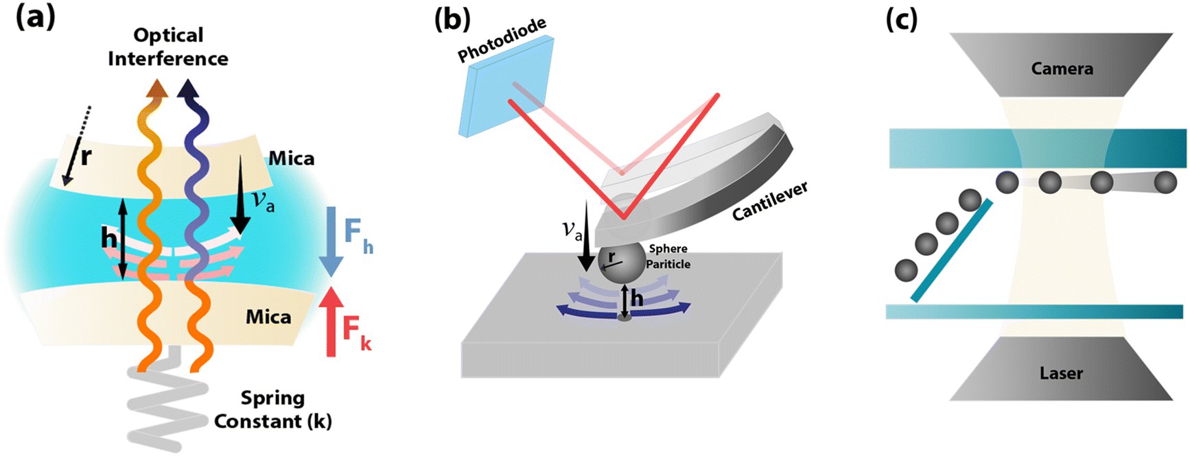
NEMD simulations have been applied to determine the friction coefficient and LS for different solid–liquid interfaces. A key aspect of NEMD simulations is the application of a gradient across the computational domain to observe the system's linear response. The variables of interest are monitored over time, and once a quasi-steady state is achieved, transport or interfacial properties can be determined by fitting the data to a continuum-based model, typically involving a gradient. While the NEMD method is conceptually straightforward and closely mimics real experimental setups, it is significantly influenced by the size of the simulation box and the large gradients needed to extract statistically significant information, the latter due to the limited time scales accessible in MD simulations. Additionally, defining the location of the solid–liquid interface is paramount for performing the velocity extrapolation needed to compute LS in the NEMD model. Karim et al.95 reported that LS and η calculations, based on a solid–liquid interface defined at the first hydration layer, closely matched predictions from the modified Hagen–Poiseuille equation.For the analysis of nanochannel flow, NEMD simulations that resemble Couette and Poiseuille flows have been used. NEDM simulations consider flow between parallel plates, due to the restrictions imposed by the utilization of periodic boundary conditions in MD simulations. Generally, the simulations involve confining liquid molecules between solid walls and applying an external force to induce unidirectional motion of the liquid particles. To create Couette flow, one wall is moved at a constant speed while the other remains stationary,96–101 or both walls are moved in opposite directions,102–106 see Fig. 4. Couette flow is generally preferred for slippage and solid–liquid friction investigations due to its straightforward implementation and the constant shear rate observed over the whole liquid domain.
 | ||
| Fig. 4 NEMD methods for generating Couette flow, (a) moving walls in opposite directions and (b) moving one wall while keeping the other wall fixed. | ||
Poiseuille flow simulations are used for more general purposes, such as studying the size effect on hydrodynamic slip107 and the characterization of flow regimes in nanochannels.108,109 Unlike Couette flow, the Poiseuille flow in NEMD can be modeled in several ways. One common approach involves applying an external force to the liquid particles within a defined region, often referred to as the inlet,110,111 and allowing the system to reach equilibrium to achieve a parabolic velocity profile, as shown in Fig. 5(a). An optimization of this method proposed by Ge et al.,112 considers the addition of an external force to the fluid particles in region B, and then the velocity is rescaled in region C to generate a constant inlet temperature every time the fluid moves between periodic boundaries from outlet to inlet, see Fig. 5(b). Another method to create a pressure-driven flow, introduced by Zhang et al.,113 involves confining fluid particles with three walls; one stationary at x = 0 and two moving walls advancing at a constant speed perpendicular to the stationary one, as illustrated in Fig. 5(c). This approach successfully produces a parabolic velocity profile and a linear correlation between the mean velocity and pressure drop. Lastly, Poiseuille-like flow can be generated by applying a constant force on every liquid atom in the desired direction of flow,107–109,114,115 see Fig. 5(d). Although this method does not resemble a pressure-driven flow but a body-force-driven flow, the outcome regarding the velocity profile and shear rates are similar.116
 | ||
| Fig. 5 NEMD methods for generating a Poiseuille flow: (a) inlet-driven flow where an external force and thermostat are applied in the same finite region (based on the methodology used in ref. 110 and 111), (b) optimized inlet-force-driven flow (based on the methodology used in Ge et al.112), (c) pressure-driven flow using three walls (based on the methodology used in Zhang et al.113), and (d) driving force applied to each liquid particle (based on the methodology used in ref. 107–109, 114 and 115). | ||
To calculate LS, a velocity profile is obtained from the particle trajectories. This is done by dividing the liquid region into segments (bins), each one recording the streamwise velocity of individual atoms, see Fig. 6. These velocities are then averaged per bin and over multiple timesteps to accurately delineate the velocity profile. The resulting profile is modeled based on the type of flow (shear-driven or pressure-driven) using either a linear or parabolic function. The slip velocity is determined by extrapolation to the wall or any other characteristic length (usually one molecular diameter from the wall). Finally, LS is calculated as:
 | (6) |
 | ||
| Fig. 6 NEMD methodology to generate velocity profiles using discrete bins for (a) Couette flow (linear profile), and (b) Poiseuille flow (parabolic profile). | ||
NEMD simulations of nanochannel flow are intuitive for implementation and analysis. Unfortunately, the high shear rates necessary to dampen the numerical noise, are significantly larger than the experimentally accessible shear rates. Consequently, the work done by the external forces produces viscous heating in the liquid particles, which is a collateral effect. To avoid this problem, many authors have applied the following methods: thermostating the liquid atoms while keeping the solid atoms frozen;96–98,113,118,119 thermostating all particles;96,98,99,102 thermostating the fluid particles only in the perpendicular direction of flow (solid atoms are either mobile or inert);101,103,104,116,120–124 and thermostating only the solid atoms so they can act as natural heat sinks to remove viscous heating.107–110,114,115,125–129 Notably, most of the earlier NEMD nanochannel flow simulations employed the liquid thermostating method or all-particles-thermostating method due to the low computational cost of these strategies. Moreover, most of these investigations were concerned with the calculation of LS in uniform temperature flows. Alternatively, the few early works where the solid thermostating method was applied were concerned with the relationship between heat dissipation and hydrodynamic slip.
The discussion of the thermostating approach is amply reported in the literature. Martini et al.106 carried out multiple simulations to investigate the hydrodynamic behavior of a nanoconfined fluid under different shear rates. The main finding of this investigation was that when the liquid atoms are subjected to thermostating and the solid wall atoms remain frozen, LS increases exponentially with shear rate; conversely, if the solid atoms are thermostated and allowed to vibrate, the LS growth is bounded to a constant value at high shear rates. Ho et al.99 indicated that either thermostating the liquid or the solid was consistent with experimental conditions of high and moderate heat dissipation, respectively. They also observed that the use of different thermostats on the fluid did not affect the velocity profiles.
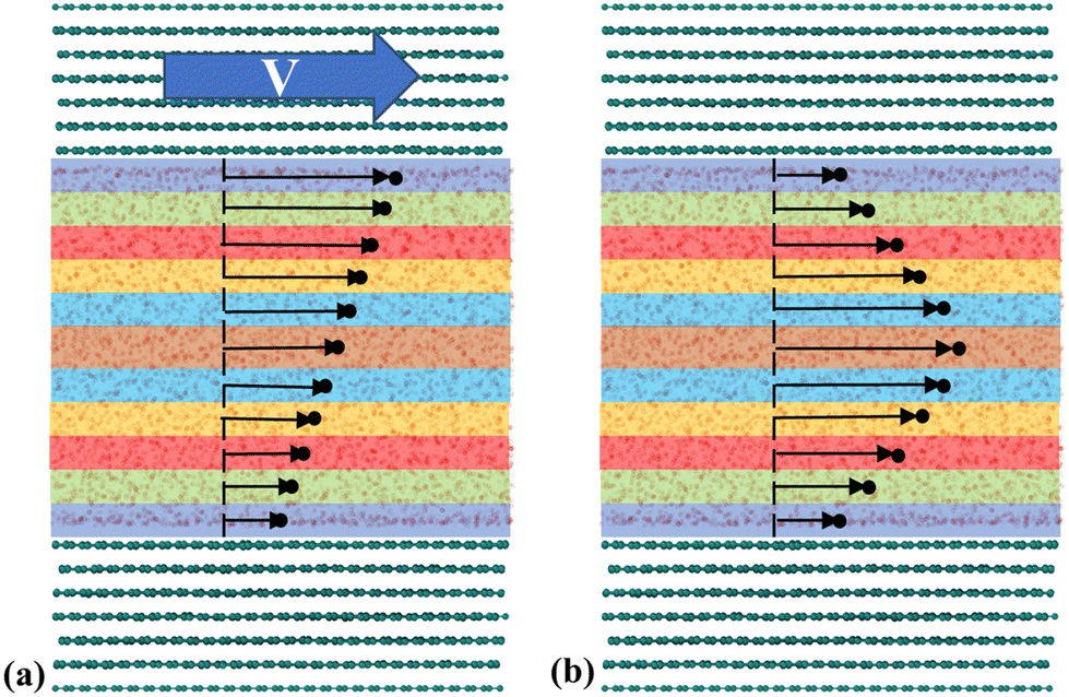
In a more in-depth investigation, Bernardi et al.130 indicated that thermostating could alter the flow physics if not applied correctly to a system where inhomogeneities exist, such as in nanochannel flow. Two scenarios were considered using a 2-D Couette flow: (1) thermostating the fluid particles while keeping the solid atoms "frozen" and (2) thermostating the solid atoms while allowing the liquid to heat up. The first finding was that the properties of the wall affect the density profiles. If the solid walls are allowed to vibrate, the liquid can slightly push the walls and make the channel effectively bigger. Moreover, thermostated fluids presented unrealistic shear distribution curves, which were not consistent with theoretical expectations. The effect of the wall atom dynamics was like that observed by Martini et al.,106 showing that at low shear rates, the vibrating walls allowed larger slip than frozen walls. The wall dynamics effect was explained by looking at the elasticity of particle collisions using rigid and flexible walls (tethered by elastic springs). Depending on the collision angle, a rigid wall limits the direction of motion of a liquid particle post collision, whereas an elastic wall allows for liquid particles to easily move in the direction of flow after a collision (see Fig. 7(a) for the schematic of rigid and flexible wall types).
 | ||
| Fig. 7 (a) Schematic of rigid and flexible walls interacting with liquid particels in NEMD models, (b) temperature profile obtained by Shuvo et al.129 (this figure has been adapted from ref. 129 with permission from AIP publishing, copyright 2024). | ||
Yong and Zhang131 performed a series of MD simulations with three different thermostat setups: (i) applying the thermostat only to liquid atoms, (ii) applying it to both solid and liquid atoms, and (iii) applying it solely to solid atoms. They investigated the mechanical and thermal properties of the system for each setup. Their findings showed that using a thermostat on the solid walls resulted in a parabolic temperature profile, which aligned with the solution of the energy equation. However, deviations from theoretical expectations occurred when isothermal conditions were applied to the liquid atoms at high shear rates. Similarly, Shuvo et al.129 applied thermostating to the walls only to mimic natural cooling, and observed a parabolic temperature distribution in the nanochannel consistent with theoretical expectations, as illustrated in Fig. 7(b). It can be concluded that allowing for wall heat dissipation, as it would naturally occur, is preferred over direct liquid thermostating.
As previously discussed, the most realistic manner of performing NEMD simulations of nanofluidics is by thermostating the wall atoms to allow the liquid to expel the excess viscous heating through the walls; however, a significant computational demand is inherent to this approach, i.e., the equations of motion must be solved for the solid particles too. Bernardi et al.130 and recently De Luca et al.,132 proposed a novel methodology for conducting physically realistic simulations without solving the dynamics of the wall. This is a new thermostating method that uses virtual particles that only interact with the liquid while being tethered to their lattice site via an elastic spring model, see Fig. 8. The wall particles are rigid, while virtual particles serve as heat sinks. Although this method was proven to be efficient and did not significantly alter the dynamics of the flow, several trial runs must be conducted before finding the most appropriate configuration (number and position) of virtual atoms for a particular system.
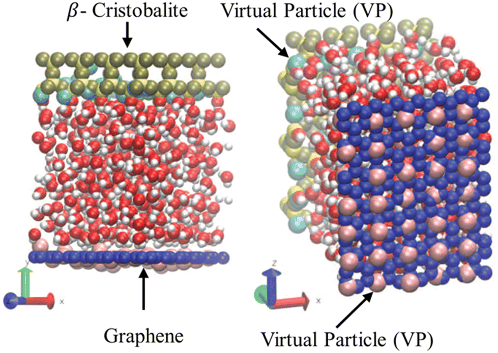 | ||
| Fig. 8 Computational domain of water confined between graphene sheets (dark blue spheres) and β-cristobalite (yellow spheres) wall with virtual particles (pink and light blue spheres). This figure has been adapted from ref. 133 with permission from American Chemical Society, copyright 2014. | ||
4.2 Equilibrium molecular dynamics (EMD)
EMD simulations are used to calculate the friction coefficient at solid–liquid interfaces without relying on creating a non-equilibrium condition, either from flow-driven or pressure-driven setups. These methods do not resemble experimental setups as in NEMD, but are more reliable than NEMD simulations for systems with large values of slip, such as water flowing in carbon nanochannels,127 where the velocity profiles are difficult to resolve. Notably, EMD methods often match NEMD calculations of slip in the low shear regime. The calculation of the friction factor using EMD is based on the fluctuation-dissipation theory, which leads to Green–Kubo-like expressions. The fluctuation-dissipation of particle forces, velocities, and their cross-correlations have been used to determine the friction factor employing four principal methods that are discussed herein.Bocquet and Barrat118 proposed avoiding the arbitrariness of choosing the hydrodynamic boundary conditions by performing first-principles calculations. A “phenomenological” model of momentum transport based on the Navier–Stokes equations was formulated using a statistical mechanics approach, selecting LS and the hydrodynamic distance to the wall (zwall) as fitting parameters. Analytical expressions for the momentum density correlation function were obtained for perfectly flat and rough walls. MD simulations were performed to obtain the “exact” values of the momentum density correlation function. Equilibrium simulations of nano-confined atomic liquids interacting through purely repulsive potentials were conducted at constant temperature and varying the size of the channels. Through parameter fitting, Bocquet and Barrat118 calculated LS and zwall, and found that the analytical models matched the simulation results for repulsive walls with and without corrugation. However, confinements imposed by attractive walls were not correctly described by the phenomenological model due to the presence of slip-locking. Lastly, they conducted NEMD simulations of Couette flow to prove the effectiveness of the “phenomenological” model in predicting the velocity profile. The analytical model fitted through EMD simulations accurately matched the NEMD velocity profiles.
Given the success of their equilibrium calculations, Bocquet and Barrat118 formulated a method to calculate LS and zwall as equilibrium properties using a Green–Kubo-like approach. They employed linear response theory and the Mori–Zwanzig formalism separately to derive equilibrium coefficients based on the time-dependent correlation functions of the fluid. A perturbation Hamiltonian  was chosen to generate a Poiseuille flow in the x-direction with a fictitious shear field
 ![[small gamma, Greek, dot above]](https://www.rsc.org/images/entities/i_char_e0a2.gif) , where Pi,x is the momentum of particle i in the x-direction, and z0 is the position at which the velocity profile vanishes while vx(z) = (z − z0) is a first-order approximation of the tangential velocity. Applying linear response theory with a non-equilibrium friction force 〈Fx〉(t) as the response and H as the perturbation field, the following expression was developed:
, where Pi,x is the momentum of particle i in the x-direction, and z0 is the position at which the velocity profile vanishes while vx(z) = (z − z0) is a first-order approximation of the tangential velocity. Applying linear response theory with a non-equilibrium friction force 〈Fx〉(t) as the response and H as the perturbation field, the following expression was developed:

 | (7) |
 | (8) |
 | (9) |
According to Navier's friction model,46Fx = −λAvx(Δz), where Fx is the total tangential force exerted by the liquid on the wall and νx(Δz) is the tangential velocity at an equilibrium position Δz away from the wall; Bocquet and Barrat118 assumed that (z0 − zwall) = vx(Δz) to find an expression for the friction coefficient. Petravic and Harrowell134 indicated the incorrectness of such an assumption given that is an artificial constant field used to introduce a perturbation to the system and no physical correlation exists with Fx which is the friction force on the wall.
Petravic and Harrowell134 addressed the equilibrium perturbation issue using Doll's equations of motion. They induced a disturbance within the system by generating a relative velocity, referred to as Δvwall, between the confining walls, while also considering the constraints of a heterogeneous system in a boundary-driven flow context. The system's linear response was then evaluated in the context of a small Δvwall, leading to the determination of a new friction coefficient.
 | (10) |
 | (11) |
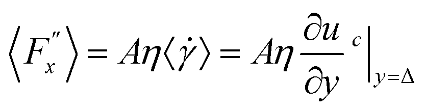
Hansen et al.125 emphasized that eqn (9) accounts for the friction of the whole system, including both the walls and the liquid, and highlighted the importance of separating the region affected by the wall from the bulk fluid to accurately determine the true wall friction. They expanded on Navier's foundational ideas, addressing the issue of wall friction by focusing on a thin layer of liquid close to the wall, see Fig. 9. The analysis considers the velocity profile of a liquid confined between two walls, separated by a distance Ly, where the liquid slab delimited at y = Δ is analyzed using Newton's second law:
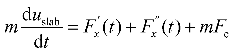 | (12) |
 , whereas
  is the friction force due to the fluid-slab interactions. Lastly, Fe is an applied external force per unit mass.
 | ||
| Fig. 9 Sketch of the system used in the friction analysis in Hansen et al.125 This figure has been redrawn from ref. 125 with permission from American Physical Society, copyright 2011. | ||
The friction force  was described by the following expression:
 | (13) |
 represents a random force that has a zero mean and is uncorrelated with uslab. In steady-state conditions, the friction forces are given as:
 | (14) |
 | (15) |
 | (16) |
 | (17) |
And
 | (18) |
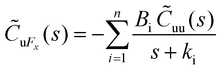
The Laplace transform of the friction kernel was obtained using a Maxwellian memory function for convenience as indicated in Hansen et al.,125
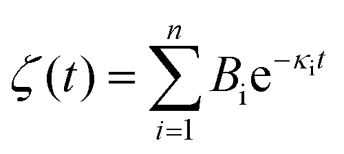 | (19) |
Thus, the zero-frequency friction coefficient can be found by fitting Bi and κi in eqn (19) using data from EMD simulations as:
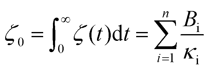 | (20) |
Hansen et al.125 discovered that ζ0 depended on Δ, requiring multiple trials to determine the appropriate Δ value. Thin slabs failed to capture the entire wall-slab interactions, while wider slabs may introduce unnecessary bulk particles. They noted that the friction coefficient was influenced by the channel width, particularly for channels with Ly ≤ 7σ, where σ denotes molecular diameter. A comparison was conducted between the LS predicted using their EMD approach and NEMD calculations using Couette and Poiseuille flows, and a remarkable agreement between the two methods was found for flows with small shear rates.
Bocquet and Barrat135 addressed the criticisms in the definition of their model reported in Bocquet et al.,118 suggesting that the sensitivity of their interfacial friction coefficient stemmed from the approach taken in handling system size and time limits extending to infinity, as derived from MD simulations. To reinforce the generality of their previous model, they introduced a new formulation for the Green–Kubo relationship for the friction coefficient λ, offering a more robust and fundamental approach grounded in the general Langevin equation. This formulation was applicable to both planar and cylindrically confined fluids. In their study, Bocquet and Barrat135 defined a confined liquid system in which solid walls of large mass M are allowed to move in the tangential direction only. In the presence of solid–liquid friction, the fluctuations in the wall velocity U(t) are given by:
 | (21) |
 | (22) |
 | (23) |
Eqn (23) is best handled in the Laplace space from which the friction coefficient was found when ![[small variant phi, Greek, tilde]](https://www.rsc.org/images/entities/char_e12c.gif) (s) is evaluated in the s → 0 limit, yielding:
(s) is evaluated in the s → 0 limit, yielding:
 | (24) |
Huang and Szlufarska123 noted a significant concern in the discourse regarding friction coefficients derived from equilibrium calculations. They argued that the friction coefficient should be considered a local parameter rather than a bulk property. For instance, while solid–liquid friction exists in liquids moving through a carbon nanotube, achieving the thermodynamic limit in such a system, as proposed by Bocquet and Barrat,118,135 is not feasible. Moreover, when dealing with heterogeneous surfaces or fluid mixtures in contact with a solid boundary, using a bulk property equation like eqn (24) fails to capture the localized variations at the interface where friction takes place. Bocquet et al.135 applied the general Langevin equation along with a set of sum rules to the fluctuating velocity of a wall of large mass. In a new formulation, Huang and Szlufarska123 applied a mechanical perturbation Hamiltonian to individual liquid particles at the solid–liquid interface, H = −xfeiωt where x is the displacement of particles parallel to the solid walls and feiωt is an external drag force with frequency ω and time t. Being ui the drift velocity of an interfacial particle moving parallel to the solid wall, and Fourier transforming the linear correlation function, the particle's drift velocity and mobility ϕi were obtained as:
 | (25) |
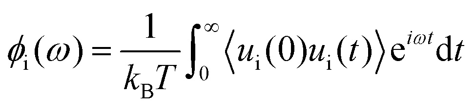 | (26) |
Linear response theory was applied a second time using Fi as the force exerted by the wall on a single interfacial particle i yielding:
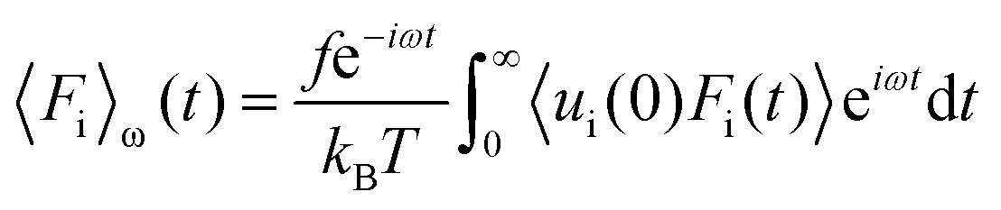 | (27) |
Now, by definition of the friction coefficient:
 | (28) |
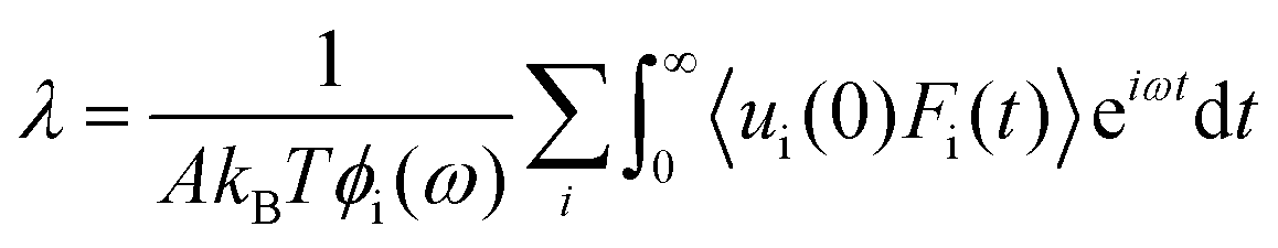 | (29) |
 | (30) |
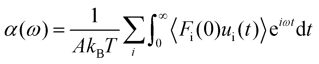 | (31) |
![[small eta, Greek, macron]](https://www.rsc.org/images/entities/i_char_e0c8.gif) (0) can be used to obtain
(0) can be used to obtain  . Table 2 summarizes the EMD models for the calculation of LS with key highlights.
| Source | Equations | Key highlights |
|---|---|---|
| Bocquet and Barrat118 |

|
• Utilized both linear response theory and the Mori–Zwanzig formalism independently to derive equilibrium coefficients. |
| • Introduced an artificial shear rate into the fluid using a Hamiltonian to simulate Poiseuille flow. | ||
| • Analyzed the ACF of the friction factor focusing on the solid atoms. | ||
| • Determined that the ACF should reach zero when t → ∞; and calculated λ at this point | ||
| Petravic and Harrowell134 |
|
• Discovered that the ACF's integral does not reduce to zero over time but instead stabilizes at a constant value, implying a smooth decay of the force ACF. |
|
• Employed a method similar to Bocquet and Barrat118 for calculating the friction factor, though they disagreed on the interpretation of the findings. | |
| • Identified that the friction coefficient varies with system size, indicating it is not an intrinsic interfacial property. | ||
| Hansen et al.125 |
|
• Proposed isolating the region near the wall from the bulk to accurately determine wall friction. |
| • Developed a dynamic analysis of a thin liquid slab adjacent to the wall, correlating the friction force with the slab velocity using a memory function. | ||
| • Conducted the ACF analysis focusing on the interfacial liquid atoms. | ||
| Bocquet and Barrat135 |

|
• Refined their earlier model to address criticisms regarding the generality of their Green–Kubo formulation. |
| • Introduced a non-Markovian general Langevin framework to investigate perturbations in the wall velocity and slip behavior. | ||
| Huang and Szlufarska123 |
|
• Applied linear response theory to a system of liquid particles subjected to perturbations by a Hamiltonian. |

|
• Assumed that particles interact independently, with interfacial interactions considered additive. | |
| • Conducted the ACF analysis on the liquid atoms. | ||
| • The model indicated that several Langevin equations are needed to explore both wall velocity and slip behavior, indicating a linear relationship between these variables. | ||
Bocquet and Barrat118 identified the deficiencies of integrating the force ACF in eqn (7) in the limit when the lag time goes to infinity. As an alternative, it was proposed to evaluate the integral only up to the point where the ACF reached its first zero. A year earlier, Español and Zúñiga136 highlighted the issues with evaluating the friction factor integral from zero to arbitrary limits as indicated in Bocquet et al.118 The solid–liquid friction phenomenon was studied using Hamilton's equation with projection operators on a Brownian particle of infinite mass interacting with other particles. Complimentary EMD simulations were carried out by analyzing a fixed liquid particle (infinite mass particle) interacting with several other liquid particles to prove a correlation between the decay of the momentum ACF and the friction factor. The force ACF decreased fast and smoothly but the integral of such was rather noisy with a tendency to decay after long simulation times. No plateau of eqn (7) was found for long simulation times, as suggested when the thermodynamic limit was reached, but approximations of the friction factor could be extracted from shorter-time behaviors.
Español and Zúñiga136 concluded that EMD calculations using Green–Kubo-like models are hindered by the order in which the thermodynamic limit (infinite number of particles) and the infinite time limit are taken since they do not commute. However, as the simulation systems get larger, it is expected that the friction coefficient calculations approach the obtained results in the limits discussed. Notably, several authors reported no issues with the evaluation of eqn (7).36,116,117,128,134 In these investigations, smooth time-dependent friction factors are reported with a plateau at which point the steady state friction factor is evaluated. Furthermore, consistency between EMD calculations using eqn (7) and NEMD has been reported.116,117,128 Liang and Keblinski128 obtained the friction factor of argon flowing between graphene surfaces and observed a steady friction factor plateau over a window of 12 ps analyzing data over 10 ns.
Tocci et al.36 used ab initio MD and force field MD simulations to obtain the friction factor for graphene and hexagonal boron nitride in contact with water. By using both sources of atomic trajectories evaluated from 50 ps to 10 ns in a 1 ps time window, they obtained smooth friction coefficient integrals. Falk et al.117 evaluated the friction factor from force ACFs evaluated over 0.4 ns with a time window of 2 ps. It was indicated that at long timescales (typically nanoseconds), the integral vanishes due to the finite size of the system, but at intermediate times a plateau of the integral can be observed. Additionally, they did not observe confinement dependence on the friction factor. Contrariwise, Wei et al.116 used eqn (7) to determine the LS in water confined between graphitic-carbon walls and observed a confinement effect on the friction coefficient after the viscosity was adjusted to the confinement level. The investigation by Harrowell and Petravic134 focused on giving a better interpretation of eqn (7) and throughout their analysis, smooth time-dependent friction coefficients were observed. Contrarily, Huang and Szlufarska123 observed rather fluctuating time-dependent friction coefficient graphs.
Arguments supporting and disproving the properties of the original friction coefficient expression derived by Bocquet and Barrat118,135 can be found all over the literature. The vanishing behavior of the integral in eqn (7) has been consistently reported. Likewise, the confinement effect has been reported by some authors, but others did not capture that in their analysis. New analytical approaches and reinterpretations of the initial model have been proposed, but they have not been widely investigated. For example, only Kannam et al.126,127 used the method, proposed by Hansen et al.,125 to study the friction between liquids and graphite surfaces obtaining consistent results with NEMD simulations in the low shear rate limit. There is a notable debate surrounding the EMD analysis of hydrodynamics in nanoconfined liquids, and more comprehensive studies are necessary to reach definitive conclusions. The methodologies for analysis and simulation are not thoroughly detailed in existing literature, and the inconsistencies observed across various studies may stem from errors in postprocessing or data sampling during EMD simulations.
5 The hydrodynamics of nanoconfined flows
5.1 Hydrodynamic slip mechanisms and molecular origins
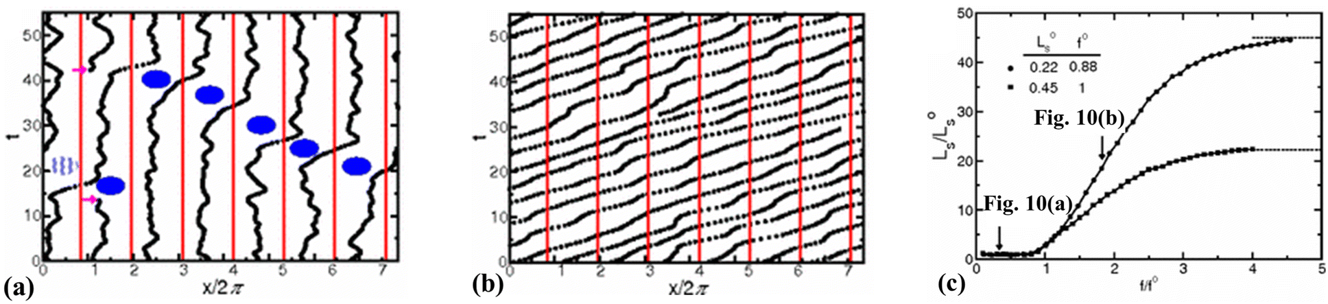
Thompson and Robbins98,137 made significant contributions to the understanding of the stick-slip mechanisms of liquids moving past solid surfaces by examining this phenomenon from a thermodynamic standpoint rather than considering it as a hydrodynamic instability. Through NEMD simulations of Couette flow, they recorded the friction force, wall displacement, and structure factor over time as the wall velocity varied. Their findings revealed that increasing the binding strength between solid and liquid atoms led to solid-to-liquid transitions in the liquid particles at the interface. In some extreme cases, crystallization of interfacial liquid particles occurred, which was then disrupted by the high shear stresses present in the Couette flow. This interplay between solid–liquid binding and shear-induced disruption resulted in periodic phase transitions, thereby framing hydrodynamic slip within a thermodynamic context.Lichter et al.138 proposed that liquid molecules spend sufficient time near the wall to warrant a dynamic treatment of their molecular motion, based on the observed ordering of liquid particles in the direction perpendicular to the wall and the mass flux towards the solid. They developed a stochastic differential-difference equation for particles in the first adsorption layer near the wall, allowing for mass exchange between the bulk and interfacial particles. This approach was termed the variable-density Frenkel-Kontorova model (vdFK). The vdFK model was qualitatively successful in predicting the relationship between shear rate and LS observed in NEMD simulations. Moreover, the model identified two distinct slip mechanisms observed in NEMD simulations: (1) slip caused by localized defect propagation, where particle exchange occurs between interfacial vacancies and the bulk, and (2) simultaneous slip of large liquid regions. At low shear rates, localized defects emerge within the liquid layer, with adjacent molecules quickly filling the resultant vacancies, as depicted in Fig. 10(a). This defect propagation is notably slow under low-shear conditions. In contrast, at high shear rates, the shear forces are sufficient to induce concurrent slip across large domains of the liquid layer, see Fig. 10(b). Fig. 10(c) illustrates the response of LS to the applied force as modeled by the vdFK model, demonstrating that at low levels of force, LS remains relatively constant. This stability is due to the sparse nature of molecular defects, which propagate slowly through the adsorbed liquid layer without significantly affecting the overall slip behavior. These defects do not cover a substantial area, thus minimally impacting the bulk liquid behavior. However, as the force increases, a sharp transition occurs due to the intensification of local defects. Ultimately, the system reaches a new plateau at higher applied forces, indicating that the liquid layer moves uniformly over the solid surface. Further increases in force do not significantly impact the LS, suggesting a saturation of mobility mechanisms at the interface.
 | ||
| Fig. 10 Trajectories of liquid atoms predicted by the vdFK model, (a) at a low shear rate (defect propagation stage), and (b) at a high shear rate (translation of the entire first liquid layer or concurrent slip). The black solid dots represent the positions of liquid atoms at the interface. For an eye guide, the blue dots indicate the generating vacancies and filling the resultant vacancies. The vertical red solid lines illustrate the positions of seven solid atoms at the interface. (c) LS as a function of the applied force calculated from the vdFK model. The LSvs. force data were normalized to collapse the low-forcing data points onto a single curve for different ground states which denotes the ratio of liquid–liquid and solid–solid spacing. The arrows in panel (c) indicate the LS for the corresponding molecular trajectories of the panel (a) and (b). This figure has been adapted from ref. 138 with permission from American Physical Society, copyright 2004. | ||
Martini et al.139 reported defect slip (like in the vdFK model) using low shear rate NEMD simulations. In this regime, liquid particles adjacent to the solid surface hop between equilibrium sites within a potential field generated by the solid following Arrhenius dynamics. At higher shear rates, they observed global slip, where the entire layer of liquid particles moves collectively. At the smallest wall velocity, atom movement was almost indiscernible, with minimal movement either upstream or downstream. As the wall velocity increased to intermediate levels (5 ms−1 and 50 ms−1), atoms displayed periods of stillness interspersed with sudden downstream shifts. At 50 ms−1, the behavior began to show collective trends where groups of atoms might slip simultaneously, indicating the onset of a more coordinated movement. At the highest wall velocity simulated, a distinct global slip was observed where all atoms within the first adsorbed liquid layer move uniformly downstream, presenting parallel trajectories that indicate a cohesive and uniform motion over the solid wall. These observations align with the vdFK model. Additionally, Martini et al.139 found a critical wall velocity for their system—a specific wall velocity that demarcates the transition from defect-driven slip to this observed global slip.
When molecular vacancies at the interface are widely spaced during liquid slip, the movement of a single atom from one equilibrium position to another happens independently. This independence allows for studying the dynamics of individual atoms and the application of transition-state theory.139 Babu and Sathian120 utilized Eyring's theory of reaction rates (transition-state theory), which models viscous flow as a chemical reaction where the primary process involves molecular hopping between equilibrium positions, see Fig. 11. In this context, liquid molecules must surpass an energy barrier created by neighboring molecules to reach a new equilibrium position. A comprehensive analytical model comprising six equations was developed, with shear viscosity and the friction coefficient being the primary outputs. NEMD simulations of water confined between graphene sheets and carbon nanotubes (CNTs) were conducted to directly compute the friction coefficient and estimate the activation energy of the liquid molecules—an essential input for the analytical model. The model's validity is contingent upon maintaining a low shear rate to ensure defect slip, as noted by Martini et al.139 The friction coefficient predictions from the analytical model generally aligned with the numerical simulations, although there were instances of underestimation and overestimation for the various confinement levels studied. The authors indicated that they used different driving forces, in a Poiseuille flow configuration, and varied the channel dimensions. If this process is not performed carefully, markedly different shear rates would be produced if the driving force is kept constant while the channel size varies. Additionally, Babu and Sathian120 found size-dependent friction coefficients for flow between graphene sheets but Falk et al.117 reported otherwise.
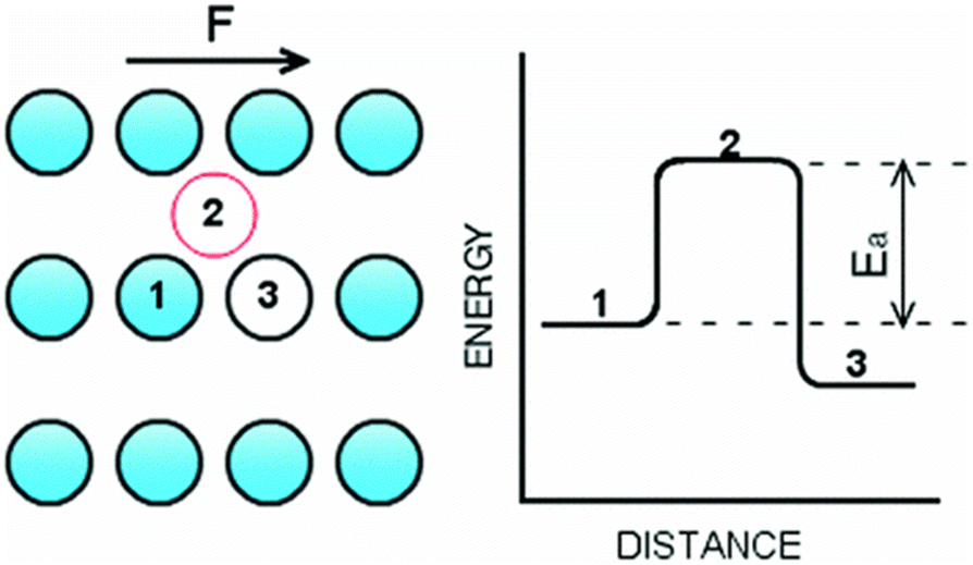 | ||
| Fig. 11 Schematic of atom transition from one equilibrium position to another following Eyring's theory of reaction rates. The figure has been adapted from ref. 120 with permission from American Physical Society, copyright 2012. | ||
Understanding friction forces at solid–liquid interfaces remains a significant challenge. For instance, Tocci et al.140 investigated the friction of water at the interfaces of graphene and hexagonal boron nitride (h-BN) using ab initio molecular dynamics (AIMD) simulations. Notably, graphene and h-BN generated a similar interfacial water structure. Furthermore, the AIMD calculations revealed nearly identical contact angles for water droplets on graphene and h-BN sheets.141 Despite interfacial liquid structure and wettability similarities, the calculated friction coefficient on h-BN was approximately three times higher than on graphene. This significant difference was attributed to the greater corrugation of the energy landscape generated by h-BN, determined by the differences in the electronic structure of the two 2-D materials. To further investigate this phenomenon, Secchi et al.142 conducted experiments on water transport inside carbon nanotubes (CNTs) and boron nitride nanotubes (BNNTs). Their study revealed a significant radius-dependent slippage in CNTs, where water flowing through the nanotubes exhibits nearly frictionless interfaces, leading to exceptionally high flow rates. In contrast, BNNTs showed almost no slippage, despite their similar crystallography to CNTs. This difference highlights the influence of subtle atomic-scale interactions at the solid–liquid interface, suggesting a connection between hydrodynamic behavior and the electronic properties of the confining material.
Recently, Kavokine et al.143 developed a quantum theory of the solid–liquid interface and introduced a new concept of quantum friction caused by the coupling of charge fluctuations in water to electronic excitations in the solid surface. In this theory, the authors argued that hydrodynamic friction arises not only from the static roughness of a solid surface (classical friction) but also from the interaction between water fluctuations and solid electronic excitations (quantum friction). Thus, this concept could be understood from the electronic contribution to the solid–liquid friction behavior. They also investigated water interactions with graphitic materials, where (i) graphene, a 2-D material, exhibited very low energy excitations at very small momenta (q ≤ 0. 02 Å−1); suggesting that the electronic excitations in graphene are less likely to interact with water molecules over large distances, contributing negligible quantum friction compared to classical friction. Conversely, (ii) graphite exhibits unexpectedly high friction compared to graphene caused by the distinct electronic structure due to the coupling between its layers; this coupling leads to the emergence of low-energy plasmon modes in graphite, which are absent in single-layer graphene. These low-energy excitations, particularly the surface plasmon modes, strongly interact with water molecules at the interface. In graphite, the low-energy plasmon mode has a frequency of approximately 50 meV and is polarized perpendicularly to the layers. This mode has a flat dispersion over a range of momenta, meaning it can interact more effectively with the fluctuating electric fields of water molecules, particularly with the Debye mode of water. The strong interaction between the graphite plasmon modes and the water Debye mode leads to enhanced quantum friction at the interface. Thus, the overall friction at the graphite-water interface is higher than at the graphene-water interface. Furthermore, Bui et al.144 applied a classical model that adjusts the dielectric properties of a solid using a simple model of charge density fluctuations in a carbon substrate. Their findings showed an increase in interfacial friction consistent with recent theories of quantum friction, with friction rising as the solid's dielectric spectrum features overlap with the librational and Debye modes of water.
5.2 Solid–liquid affinity characterized via wettability and liquid structuring effects on slip
In nanoconfined liquids, surface effects are predominant and one of the most significant is the solid–liquid affinity. A macroscopic outcome of such affinity can be characterized using the contact angle (surface wettability). From an experimental point of view, it is very difficult to change the wettability of a surface; however, MD simulations offer several options to do this, e.g., (i) modifying the solid–liquid atomic force field, (ii) manipulating the electrostatic interactions between solid and liquid particles, (iii) varying the surface atomic density, and (iv) modifying the simulation temperature. Although these simulations are limited to atomically smooth surfaces, important investigations have been conducted in this area.145–147Voronov et al.96,97 used standard EMD simulations to determine the contact angle of a simple Lennard-Jones (LJ) fluid on a graphite-like solid (i.e., droplet wettability). A parametric analysis was conducted in which the solid–liquid LJ parameters were independently varied to assess their effects on the calculated contact angle. Increasing the value of the solid–liquid energy parameter (εsl) generated more hydrophilic surfaces and prompted liquid particles near the wall to mimic the wetted solid structure, as reported by Thompson et al.98 A linear dependence of the contact angle on εsl was found. Alternatively, the LJ length parameter (σsl) produced changes in the surface energy landscape. Larger values of σsl mimicked smoother and more hydrophilic surfaces than smaller values of this parameter, similar observations are reported by Zhang et al.124 Thus, two opposite trends were found depending on how the surface wettability is altered, and caution was advised for modeling slip surfaces. LS increased as the contact angle increased when one modifies εsl; however, LS decreased as the contact angle decreased when σsl was increased. Two different mechanisms are responsible for such behaviors, one is pertinent to a binding energy effect (εsl), and the other is relevant to the surface energy landscape granularity (σsl). Hydrophilic surfaces generated by smooth energy landscapes cause large slip; alternatively, hydrophilic surfaces generated by strong solid–liquid affinity led to small slip. Thus, liquids can slip over hydrophilic surfaces and hydrophobic surfaces can have minimum slip if the surface energy landscape allows for liquid particles to be trapped.
L
S is greatly influenced by the magnitude and type of the solid–liquid force field parameters, which define the interface affinity. Previous investigations correlated LS at various interfaces to surface wettability. In a significant development, Huang et al.103 made an important contribution by proposing a quasi-universal scaling relation that suggests that LS is a function of wettability, LS∼ (1 + cos![[thin space (1/6-em)]](https://www.rsc.org/images/entities/char_2009.gif) θ)−2, where θ denotes the contact angle, see Fig. 12(a). Ho et al.99 challenged this relation by modifying the wettability of MgO through adjustments to its lattice constant, finding that LS increased in more hydrophilic surfaces. In a related study, Wang et al.148 used MD simulations and AFM experiments to determine the friction coefficient at various solid-water interfaces. Their findings revealed a significant limitation of using the contact angle alone to explain variations in friction coefficients at the nanoscale. Despite observing a similar contact angle, the friction coefficient increased 41 times as the surface charge increased from 0e to 0.36e. This rise in friction was attributed to localized potential energy fluctuations, which create additional energy barriers for water molecules, underscoring the limitation of wettability metrics to explain the friction coefficient and hydrodynamic slip in nanochannels. Wang et al.149 further investigated the role of ordered water molecules at the solid–liquid interface of superhydrophilic surfaces using NEMD simulations. They observed that the formation of a hexagonal-like structure in the first water monolayer significantly reduced friction between the monolayer and bulk water above by decreasing the number of hydrogen bonds. The weakened hydrogen bonding led to smoother interlayer movement, thereby considerably reducing the overall friction at the interface. Supporting these observations, Xu et al.150 conducted MD simulations in different polygonal carbon nanotubes (CNTs), demonstrating a similar frictional reduction due to the ordering of water molecules in the first monolayer.
θ)−2, where θ denotes the contact angle, see Fig. 12(a). Ho et al.99 challenged this relation by modifying the wettability of MgO through adjustments to its lattice constant, finding that LS increased in more hydrophilic surfaces. In a related study, Wang et al.148 used MD simulations and AFM experiments to determine the friction coefficient at various solid-water interfaces. Their findings revealed a significant limitation of using the contact angle alone to explain variations in friction coefficients at the nanoscale. Despite observing a similar contact angle, the friction coefficient increased 41 times as the surface charge increased from 0e to 0.36e. This rise in friction was attributed to localized potential energy fluctuations, which create additional energy barriers for water molecules, underscoring the limitation of wettability metrics to explain the friction coefficient and hydrodynamic slip in nanochannels. Wang et al.149 further investigated the role of ordered water molecules at the solid–liquid interface of superhydrophilic surfaces using NEMD simulations. They observed that the formation of a hexagonal-like structure in the first water monolayer significantly reduced friction between the monolayer and bulk water above by decreasing the number of hydrogen bonds. The weakened hydrogen bonding led to smoother interlayer movement, thereby considerably reducing the overall friction at the interface. Supporting these observations, Xu et al.150 conducted MD simulations in different polygonal carbon nanotubes (CNTs), demonstrating a similar frictional reduction due to the ordering of water molecules in the first monolayer.
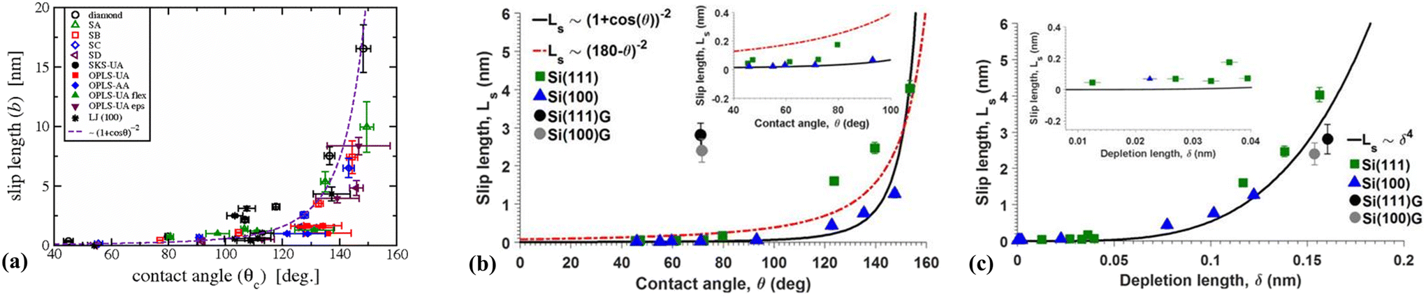 | ||
| Fig. 12 (a) Quasi-universal relationship, where LS is a function of contact angle, proposed by Huang et al. The panel (a) has been adapted from ref. 103 with permission from American Physical Society, copyright 2008. LS of Si and graphene-coated Si channels as a function of (b) the contact angle, and (c) the density depletion length δ. The (b) and (c) panels have been adapted from ref. 151 with permission from AIP publishing, copyright 2016. | ||
These findings indicate that friction and hydrodynamic slip at the solid–liquid interface are affected by the liquid structuring at the interface rather than by wettability. To quantify this phenomenon, recent investigations introduced the concept of density depletion length (δ),93,103,104,151 which quantifies the presence (excess/deficit) of momentum-carrying liquid molecules at the interface (see Fig. 3c). The following equation has been reported to calculate δ:
 | (32) |
In addition to a quasi-universal relationship, Huang et al.103 and Sendner et al.104 reported that LS correlates with the density depletion length as LS∼ δ4. This scaling law is based on analyses using a mean-field theory model of wettability and a Green–Kubo-like model of slip, effectively explaining LS behaviors across different models. Ramos-Alvarado et al.,151 in their series of EMD simulations on various Si nanochannels (bare Si (100) and Si (111)), and graphene-coated Si, noted that the quasi-universal relationship to θ only traced the data trends with limited fidelity and broke down for graphite-coated Si surfaces, as illustrated in Fig. 12(b). However, the scaling law of δ reliably quantified LS across these diverse nanochannels, see Fig. 12(c).
In more detailed studies, Paniagua et al.93 utilized a range of Lennard-Jones (LJ) parameters to model graphite-water interactions through EMD simulations. They reported that surface wettability was inadequate in characterizing LS. Despite accurately controlling the surface wettability in their MD simulations (symbols inside the rectangular box in Fig. 13(a)), considerable variations in LS were observed—26.87 nm, 42.61 nm, and 62.48 nm. These slip variations existed even when the contact angle, binding energy, and work of adhesion were similar across the three highlighted interfaces. This variability, driven by different friction coefficients, highlights the inadequacy of using wettability metrics alone to explain hydrodynamic slip behavior. Conversely, as depicted in Fig. 13(b), δ effectively captured the variations in LS calculated via EMD across the different interface models, where wettability metrics fell short.
 | ||
| Fig. 13 L S as a function of (a) the contact angle and (b) density depletion length. The (a) and (b) panels have been adapted from ref. 93 with permission from American Chemical Society, copyright 2020. (c) Shear-dependent LS as a function of δ. The solid and dashed lines represent the averaged LS at high and low shear rates. The (c) panel has been adapted from ref. 129 with permission from AIP publishing, copyright 2024. Each symbol represents a different interface model. | ||
Furthermore, Paniagua et al.93 noted that while the wettability scaling law could generally describe the behavior across most interface conditions, it failed in extreme hydrophobic or hydrophilic scenarios. To address this, they proposed an empirical exponential function (LS∼ eBδ) that could effectively trace LS across all graphite-water interface models. Corroborating these findings, Shuvo et al.129 conducted NEMD simulations in shear-driven flows within graphite nanochannels, confirming that the exponential function of δ also accurately describes the behavior of LS under different shear conditions, as illustrated in Fig. 13(c).
5.3 Shear rate effect on hydrodynamic slip
Shear rate is crucial in defining the boundary condition in nanoconfined liquids as the shear force on liquid particles competes with the solid–liquid binding and liquid–liquid cohesive forces. Thompson and Troian100 carried out NEMD simulations of an LJ liquid, varying parameters like εsl, σsl, and solid density using different shear rates in a Couette flow model. They observed that LS remained constant over a certain shear rate range but exhibited rapid growth beyond a critical value γc. Despite the variation in shear rates, the shear viscosity showed no significant change, indicating Newtonian behavior. A universal boundary condition was proposed: , where L0S represents the low shear rate LS limit and α is a fitting parameter, suggesting that the Navier slip condition is just a specific case of a broader relationship.
The rapid increase in LS at a critical shear rate was similarly observed in studies by Voronov et al.96,97 and Chen et al.33 in shear-driven MD simulations. Kannam et al.126 investigated hydrodynamic slip for both Poiseuille and Couette flows of graphite–argon, and graphite–methene systems, reporting an exponential (unbounded) growth of the LS in both flow types. The authors did not address the seemingly infinite growth of the LS when factors such as the wall friction coefficient and the fluid's viscosity pose a physical limit to solid–liquid friction. Wagemann et al.152 expanded on this by examining LS of water within graphene nanochannels, particularly focusing on the crystallographic directions—zig-zag and arm-chair. Their observations indicated an unbounded growth of LS in both directions, see Fig. 14(a). The authors calculated the wall friction coefficient as a function of shear rate and found that at low shear rates, the friction coefficient remained constant, indicating a stable interaction between the fluid and the solid surface. However, at high shear rates, a rapid reduction in the friction coefficient was observed, suggesting an unbounded growth of LS. Notably, the authors did not investigate the rheological properties of the liquid, which are crucial because LS is a function of both fluid viscosity and wall friction coefficient. Recently, Li et al.153 investigated the rheology of water in nanoconfined graphite walls and suggested a shear thinning effect at high shear rates.
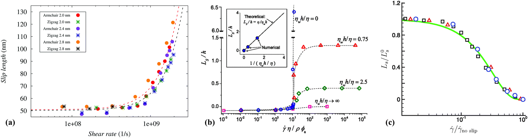 | ||
| Fig. 14 Shear effect on slip reported through the years: (a) unbounded growth of the LS, (this figure has been adapted from ref. 152 with permission from Royal Society of Chemistry, copyright 2017); (b) bounded growth of the LS, (this figure has been adapted from ref. 106 with permission from American Physical Society, copyright 2008); and (c) reduction of the LS, (this figure has been adapted from ref. 154 with permission from American Physical Society, copyright 2011). | ||
Conversely, Martini et al.139 observed different regimes of slip featuring a bounded growth of LS after a given critical shear rate, see Fig. 14(b), corroborating their molecular mechanism of slip theory. In the literature concerning the MD modeling of droplet wettability, it was reported that keeping the solid atoms rigid not only allowed to significantly reduce the computing times but also a negligible variation of the contact angle was observed compared with flexible wall models.33 Thus, several early contributions took a similar approach for their NEMD simulations of slip.96,97 Martini et al.106 hypothesized that the unbounded growth of LS with increasing shear rate, observed in previous simulations, was due to using rigid wall atoms, which overlooked momentum transfer between solid and liquid particles. To validate this, they conducted NEMD simulations of Couette flow with both fixed and flexible wall atoms. The results confirmed that rigid walls lead to unbounded LS growth at high shear rates, whereas flexible walls exhibited a constant LS beyond a certain shear rate threshold.
Pahlavan and Freund154 suggested reevaluating the high shear rate limit in NEMD simulations by decoupling the effects of the wall and thermostating approaches. Their findings indicated that the solid–liquid vibrational frequency mismatch had a negligible effect on LS, while a reduction in LS was attributed to the local temperature rise caused by an increasing number of solid–liquid collisions at high shear rates, see Fig. 14(c). Furthermore, the reduction of LS was also reported by Ramos-Alvarado et al.155 through NEMD simulation of both Couette and Poiseuille flow.
Further detailed investigations by Shuvo et al.129 using different interface models of graphite-water interfaces under different shear conditions showed a bounded growth of the LS at high shear rates, see Fig. 15(a), aligning with Martini's findings using the flexible wall model. They explored the rheology of water and the wall friction coefficient to understand the bimodal response of LS under varying shear conditions. They discovered that both viscosity and friction coefficient decreased at high shear rates but remained constant at lower shear rates, see Fig. 15(b). During the transition from low to high shear rates (LSR to HSR), the friction coefficient decreased more rapidly than the shear viscosity, until reaching a new equilibrium. As a result, the LS was higher and constant at higher shear rates.
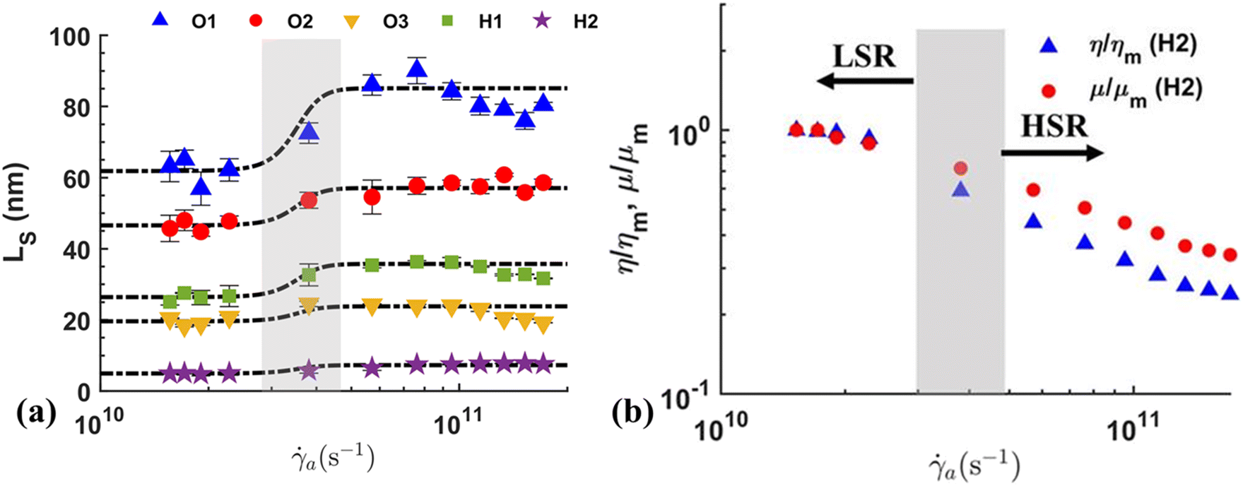 | ||
| Fig. 15 (a) The bimodal response of LS under different shear conditions. (b) Normalized viscosity and friction coefficient in shear-driven flow. The figure has been adapted from ref. 129 with permission from AIP publishing, copyright 2024. (a) was redrawn with sigmoid fits using the data reported by Shuvo et al.129 | ||
As discussed in section 4.1, NEMD simulations are pivotal in calculating the transport properties of molecular systems by mimicking experimental setups. However, achieving a good signal-to-noise ratio necessitates applying an external perturbation that is significantly larger than those typically used in experiments. This approach helps overcome the limitations of short simulation timescales and smaller length scales compared to those in experimental settings, but it also presents a challenge for directly validating the simulation results. Addressing this limitation, Maffioli et al.156 developed the TTCF4LAMMPS technique, which combines direct NEMD simulations with the Transient Time Correlation Function (TTCF). This integration facilitates the exploration of fluid responses at shear rates achievable in experiments. TTCF relies on the correlation between the initial rate of energy dissipation and the response of any phase variable following an external perturbation, described mathematically as:
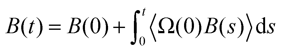 | (33) |
Despite the advantages of TTCF over traditional NEMD in terms of accessing experimentally relevant shear rates, its adoption remains limited, possibly due to the complexity of its implementation and the high computational demands associated with it.
6 Summary and outlook
Research into fluid dynamics at the nanoscale has revealed notable deviations from continuum fluid behavior, particularly regarding the phenomenologically reported no-slip condition at the solid–liquid interface. At such scales, surface effects—such as roughness, wettability, and molecular interactions—become increasingly significant due to the dimensions being on the order of molecular mean free paths. This leads to unique properties like altered viscosity and density profiles near the interface, complicating the understanding of flow dynamics.In Section 3, experimental methodologies including SFA, AFM, and μ-PIV were introduced for the direct measurement of the hydrodynamic slip length. SFA and AFM quantify the viscous drag force, which is balanced by the restorative force of the AFM cantilever based on the separation between the surface and the AFM tip. μ-PIV profiles the velocity of liquid near a solid wall by tracking particle movement. Additionally, new approaches using microchannel resonators and hybrid nanochannels with varying flow resistances were presented. These techniques are highly valuable for studying nanoscale hydrodynamic phenomena, but they also have limitations in providing detailed information on the interfacial interactions necessary to fully understand the origins of hydrodynamic slip. In Section 3.5, SFG and XRR were introduced as typical interfacial analysis techniques to study water molecules at solid surfaces. However, it remains unclear how the structural and chemical interactions of interfacial water molecules influence hydrodynamic slip behavior. These challenges have steered the field towards computational methods, where NEMD and EMD simulations play pivotal roles. NEMD simulations, which simulate shear rate effects in a manner akin to experimental setups, often require large velocity gradients to mitigate statistical noise, which can lead to unphysical conditions. Alternatively, EMD simulations focus on tracking the linear response of systems, providing a more reliable means of computing transport properties, such as interfacial friction coefficients. However, the application of Green–Kubo relations in these simulations must be handled with care to avoid introducing non-physical parameters that could skew the interpretation of nanoconfined flow characteristics.
The effect of increasing shear rate on hydrodynamic slip varies widely depending on simulation conditions, with reports of unbounded, bounded, and even reduced LS. The unbounded LS is often an artifact of simulations that neglect momentum transfer between solid and liquid particles, while reduced LS is linked to local temperature increases due to frequent solid–liquid collisions at high shear rates. The bounded growth of LS has been supported by MD simulations with flexible solid wall models where momentum transfer between solid and liquid is allowed, experiments, and theoretical models like the vdFK. Furthermore, EMD-computed LS matches with NEMD results at low shear rates. A significant limitation of traditional NEMD simulations is their reliance on very large velocity gradients. The recent development of the TCFF4LAMMPS technique enables the generation of numerical data with high signal-to-noise ratios at velocity gradients that are accessible in experiments, thereby facilitating the validation of computational models with experimental findings.
Significant advancements have been made in MD simulations unveiling atomistic details of hydrodynamic slip behavior at the solid–liquid interface, yet several fundamental questions remain unresolved. The challenge lies in developing a physics-informed boundary condition that accounts for complex interfacial interactions, including surface chemistry and interfacial liquid structuring. Current research indicates that a liquid structuring parameter may play more significant roles in hydrodynamic slip than wettability metrics, a hypothesis requiring verification. Inter-particle interactions in the liquid near the solid surface cannot be fully modeled with the parameters determined from the bulk phase properties. The solid–liquid interaction right at the interface can influence the intermolecular interaction in the next layer, which will propagate further into the liquid phase. How fast or slow this interaction decays with the distance from the surface could be another important parameter that governs (at least affects) how effectively the momentum will be transferred from the bulk liquid to the solid surface. Although indirect, such interactions could be extracted from advanced characterization methods that are sensitive to structural order or density change in the liquid phase in proximity to the solid surface. By integrating the solid–liquid interaction parameters with the boundary conditions, MD simulations will be able to predict and explain hydrodynamic slip behavior at the liquid/solid interface.
Author contributions
Abdul Aziz Shuvo: data curation (experimental and numerical part, equal), formal analysis (experimental and numerical part, equal), investigation (experimental and numerical part, equal), writing – original draft (experimental and numerical part, equal). Luis E. Paniagua-Guerra: data curation (experimental and numerical part, equal), formal analysis (experimental and numerical part, equal), investigation (experimental and numerical part, equal), writing – original draft (experimental and numerical part, equal), writing – review & editing (equal). Juseok Choi: data curation (experimental part, equal), formal analysis (experimental part, equal), investigation (experimental part, equal), writing – original draft (experimental part, equal). Seong H. Kim: data curation (experimental part, equal), formal analysis (experimental part, equal), investigation (experimental part, equal), writing – review & editing (equal), funding acquisition (equal), supervision (equal). Bladimir Ramos-Alvarado: data curation (experimental and numerical part, equal), formal analysis (experimental and numerical part, equal), investigation (experimental and numerical part, equal), writing – original draft (experimental and numerical part, equal), writing – review & editing (equal), funding acquisition (equal), supervision (equal).Data availability
No primary research results, software or code have been included and no new data were generated or analyzed as part of this review.Conflicts of interest
There are no conflicts to declare.Acknowledgements
This work was supported by the National Science Foundation, USA (Award number: 2241730), and by the Materials Research Institute at Penn State University through their Seed Grant Program.References
- C. L. Rice and R. Whitehead, J. Phys. Chem., 1965, 69, 4017–4024 CrossRef CAS.
- J. C. T. Eijkel and A. van den Berg, Microfluid. Nanofluid., 2005, 1, 249–267 CrossRef CAS.
- L. Bocquet and E. Charlaix, Chem. Soc. Rev., 2010, 39, 1073–1095 RSC.
- L. J. Guo, X. Cheng and C.-F. Chou, Nano Lett., 2004, 4, 69–73 CrossRef CAS.
- W. Sun, P. Qin, H. Gao, G. Li and K. Jiao, Biosens. Bioelectron., 2010, 25, 1264–1270 CrossRef CAS PubMed.
- V. Sunkara, B. J. Hong and J. W. Park, Biosens. Bioelectron., 2007, 22, 1532–1537 CrossRef CAS.
- P. M. Sinha, G. Valco, S. Sharma, X. Liu and M. Ferrari, Nanotechnology, 2004, 15, S585 CrossRef CAS.
- R. Lopez-Salazar, S. Camacho-Leon, L. Olivares-Quiroz and J. Hernandez, Procedia Technol., 2012, 3, 334–341 CrossRef.
- W.-H. Lee, C.-Y. Loo, D. Traini and P. M. Young, Expert Opin. Drug Delivery, 2015, 12, 1009–1026 CrossRef CAS.
- Z. Mazibuko, Y. E. Choonara, P. Kumar, L. C. Du Toit, G. Modi, D. Naidoo and V. Pillay, J. Pharm. Sci., 2015, 104, 1213–1229 CrossRef CAS.
- G. Wang, W. Mao, R. Byler, K. Patel, C. Henegar, A. Alexeev and T. Sulchek, PLoS One, 2013, 8, e75901 CrossRef CAS PubMed.
- V. Soum, S. Park, A. I. Brilian, O.-S. Kwon and K. Shin, Micromachines, 2019, 10, 516 CrossRef.
- P. Yager, T. Edwards, E. Fu, K. Helton, K. Nelson, M. R. Tam and B. H. Weigl, Nature, 2006, 442, 412–418 CrossRef CAS.
- M. L. Kovarik and S. C. Jacobson, Anal. Chem., 2009, 81, 7133–7140 CrossRef CAS.
- H. Daiguji, P. Yang, A. J. Szeri and A. Majumdar, Nano Lett., 2004, 4, 2315–2321 CrossRef CAS.
- A. Siria, P. Poncharal, A.-L. Biance, R. Fulcrand, X. Blase, S. T. Purcell and L. Bocquet, Nature, 2013, 494, 455–458 CrossRef CAS PubMed.
- B. E. Logan and M. Elimelech, Nature, 2012, 488, 313–319 CrossRef CAS.
- K.-H. Paik, Y. Liu, V. Tabard-Cossa, M. J. Waugh, D. E. Huber, J. Provine, R. T. Howe, R. W. Dutton and R. W. Davis, ACS Nano, 2012, 6, 6767–6775 CrossRef CAS.
- R. Fan, M. Yue, R. Karnik, A. Majumdar and P. Yang, Phys. Rev. Lett., 2005, 95, 086607 CrossRef.
- R. Karnik, R. Fan, M. Yue, D. Li, P. Yang and A. Majumdar, Nano Lett., 2005, 5, 943–948 CrossRef CAS.
- D. Constantin and Z. S. Siwy, Phys. Rev. E: Stat., Nonlinear, Soft Matter Phys., 2007, 76, 041202 CrossRef.
- I. Vlassiouk and Z. S. Siwy, Nano Lett., 2007, 7, 552–556 CrossRef CAS PubMed.
- R. Karnik, C. Duan, K. Castelino, H. Daiguji and A. Majumdar, Nano Lett., 2007, 7, 547–551 CrossRef CAS PubMed.
- G. Nguyen and Z. Siwy, Biophys. J., 2010, 98, 602a Search PubMed.
- R. R. Nair, H. A. Wu, P. N. Jayaram, I. V. Grigorieva and A. K. Geim, Science, 2012, 335, 442–444 CAS.
- D. Mijatovic, J. C. T. Eijkel and A. van den Berg, Lab Chip, 2005, 5, 492 CAS.
- B. Radha, A. Esfandiar, F. C. Wang, A. P. Rooney, K. Gopinadhan, A. Keerthi, A. Mishchenko, A. Janardanan, P. Blake, L. Fumagalli, M. Lozada-Hidalgo, S. Garaj, S. J. Haigh, I. V. Grigorieva, H. A. Wu and A. K. Geim, Nature, 2016, 538, 222–225 CAS.
- D. Cohen-Tanugi and J. C. Grossman, Nano Lett., 2012, 12, 3602–3608 CrossRef CAS PubMed.
- D. Konatham, J. Yu, T. A. Ho and A. Striolo, Langmuir, 2013, 29, 11884–11897 CrossRef CAS.
- A. Aghigh, V. Alizadeh, H. Y. Wong, Md. S. Islam, N. Amin and M. Zaman, Desalination, 2015, 365, 389–397 CrossRef CAS.
- K. A. Mahmoud, B. Mansoor, A. Mansour and M. Khraisheh, Desalination, 2015, 356, 208–225 CrossRef CAS.
- S. Rikhtehgaran and A. Lohrasebi, Desalination, 2015, 365, 176–181 CrossRef CAS.
- Y. Chen, D. Li, K. Jiang, J. Yang, X. Wang and Y. Wang, J. Chem. Phys., 2006, 125, 084702 CrossRef.
- M. Sega, M. Sbragaglia, L. Biferale and S. Succi, Soft Matter, 2013, 9, 8526 RSC.
- W. Song, Y. Tang, C. Qian, B. J. Kim, Y. Liao and D.-G. Yu, Innovation, 2023, 4, 100381 CAS.
- G. Tocci, L. Joly and A. Michaelides, Nano Lett., 2014, 14, 6872–6877 CrossRef CAS PubMed.
- J. K. Holt, H. G. Park, Y. Wang, M. Stadermann, A. B. Artyukhin, C. P. Grigoropoulos, A. Noy and O. Bakajin, Science, 2006, 312, 1034–1037 CrossRef CAS.
- M. Majumder, N. Chopra, R. Andrews and B. J. Hinds, Nature, 2005, 438, 44–44 CrossRef CAS PubMed.
- G. Hummer, J. C. Rasaiah and J. P. Noworyta, Nature, 2001, 414, 188–190 CrossRef CAS PubMed.
- J. A. Thomas and A. J. H. McGaughey, Phys. Rev. Lett., 2009, 102, 184502 CrossRef PubMed.
- K. Wu, Z. Chen, J. Li, X. Li, J. Xu and X. Dong, Proc. Natl. Acad. Sci. U. S. A., 2017, 114, 3358–3363 CrossRef CAS.
- J.-J. Shu, J. B. M. Teo and W. K. Chan, Soft Matter, 2016, 12, 8388–8397 RSC.
- E. Secchi, S. Marbach, A. Niguès, D. Stein, A. Siria and L. Bocquet, Nature, 2016, 537, 210–213 CrossRef CAS PubMed.
- M. Ma, F. Grey, L. Shen, M. Urbakh, S. Wu, J. Z. Liu, Y. Liu and Q. Zheng, Nat. Nanotechnol., 2015, 10, 692–695 CrossRef CAS.
- D. C. Tretheway and C. D. Meinhart, Phys. Fluids, 2002, 14, L9–L12 CrossRef CAS.
- P. M. Navier, Mem. Acad. Sci., 1823, 6, 389–440 Search PubMed.
- J. N. Israelachvili and G. E. Adams, Nature, 1976, 262, 774–776 CrossRef CAS.
- O. I. Vinogradova, J. Colloid Interface Sci., 1995, 169, 306–312 CrossRef CAS.
- D. Y. C. Chan and R. G. Horn, J. Chem. Phys., 1985, 83, 5311–5324 CrossRef CAS.
- G. Luengo, F.-J. Schmitt, R. Hill and J. Israelachvili, Macromolecules, 1997, 30, 2482–2494 CrossRef CAS.
- J. Baudry, E. Charlaix, A. Tonck and D. Mazuyer, Langmuir, 2001, 17, 5232–5236 CrossRef CAS.
- Y. Zhu and S. Granick, Phys. Rev. Lett., 2001, 87, 096104 Search PubMed.
- C. Cottin-Bizonne, B. Cross, A. Steinberger and E. Charlaix, Phys. Rev. Lett., 2005, 94, 056102 Search PubMed.
- C. Cottin-Bizonne, A. Steinberger, B. Cross, O. Raccurt and E. Charlaix, Langmuir, 2008, 24, 1165–1172 Search PubMed.
- V. S. J. Craig, C. Neto and D. R. M. Williams, Phys. Rev. Lett., 2001, 87, 054504 Search PubMed.
- O. I. Vinogradova, H.-J. Butt, G. E. Yakubov and F. Feuillebois, Rev. Sci. Instrum., 2001, 72, 2330–2339 CAS.
- O. I. Vinogradova and G. E. Yakubov, Langmuir, 2003, 19, 1227–1234 Search PubMed.
- E. Bonaccurso, M. Kappl and H.-J. Butt, Phys. Rev. Lett., 2002, 88, 076103 CrossRef PubMed.
- C. D. F. Honig and W. A. Ducker, Phys. Rev. Lett., 2007, 98, 028305 Search PubMed.
- B. Bhushan, Y. Wang and A. Maali, Langmuir, 2009, 25, 8117–8121 Search PubMed.
- A. Maali, C. Hurth, T. Cohen-Bouhacina, G. Couturier and J.-P. Aimé, Appl. Phys. Lett., 2006, 88, 163504 Search PubMed.
- A. Maali, T. Cohen-Bouhacina and H. Kellay, Appl. Phys. Lett., 2008, 92, 053101 Search PubMed.
- H. Li, Z. Xu, C. Ma and M. Ma, Nanoscale, 2022, 14, 14636–14644 Search PubMed.
- A. Maali, Y. Wang and B. Bhushan, Langmuir, 2009, 25, 12002–12005 Search PubMed.
- C. Zhang, X. Wang, J. Jin, L. Li and J. D. Miller, Colloids Interfaces, 2021, 5, 44 CAS.
- C. D. F. Honig and W. A. Ducker, J. Phys. Chem. C, 2007, 111, 16300–16312 Search PubMed.
- O. I. Vinogradova, Langmuir, 1995, 11, 2213–2220 Search PubMed.
- H. Ishida, H. Teshima, Q.-Y. Li and K. Takahashi, Int. J. Thermofluids, 2024, 22, 100634 CrossRef CAS.
- D. Lumma, A. Best, A. Gansen, F. Feuillebois, J. O. Rädler and O. I. Vinogradova, Phys. Rev. E: Stat., Nonlinear, Soft Matter Phys., 2003, 67, 056313 CrossRef CAS PubMed.
- J. Ou and J. P. Rothstein, Phys. Fluids, 2005, 17, 103606 CrossRef.
- P. Joseph and P. Tabeling, Phys. Rev. E: Stat., Nonlinear, Soft Matter Phys., 2005, 71, 035303 CrossRef.
- J. F. Collis, S. Olcum, D. Chakraborty, S. R. Manalis and J. E. Sader, Nano Lett., 2021, 21, 4959–4965 CrossRef CAS PubMed.
- Q. Xie, M. A. Alibakhshi, S. Jiao, Z. Xu, M. Hempel, J. Kong, H. G. Park and C. Duan, Nat. Nanotechnol., 2018, 13, 238–245 CrossRef CAS PubMed.
- B. Radha, A. Esfandiar, F. C. Wang, A. P. Rooney, K. Gopinadhan, A. Keerthi, A. Mishchenko, A. Janardanan, P. Blake, L. Fumagalli, M. Lozada-Hidalgo, S. Garaj, S. J. Haigh, I. V. Grigorieva, H. A. Wu and A. K. Geim, Nature, 2016, 538, 222–225 CrossRef CAS PubMed.
- J. Ping and A. T. C. Johnson, Appl. Phys. Lett., 2016, 109, 013103 CrossRef.
- A. Ambrosi, C. K. Chua, A. Bonanni and M. Pumera, Chem. Rev., 2014, 114, 7150–7188 Search PubMed.
- V. P. Zhdanov and B. Kasemo, Chem. Phys. Lett., 2011, 513, 124–126 Search PubMed.
- Q. Du, E. Freysz and Y. R. Shen, Phys. Rev. Lett., 1994, 72, 238–241 CAS.
- Y. R. Shen and V. Ostroverkhov, Chem. Rev., 2006, 106, 1140–1154 CAS.
- F. Wei, S. Urashima, S. Nihonyanagi and T. Tahara, J. Am. Chem. Soc., 2023, 145, 8833–8846 CAS.
- A. T. Celebi, M. Barisik and A. Beskok, J. Chem. Phys., 2017, 147, 164311 CrossRef.
- A. T. Celebi, M. Barisik and A. Beskok, Microfluid. Nanofluid., 2018, 22, 7 CrossRef.
- X. Geng, M. Yu, W. Zhang, Q. Liu, X. Yu and Y. Lu, Sci. Rep., 2019, 9, 18957 CrossRef CAS.
- Y. Xie, L. Fu, T. Niehaus and L. Joly, Phys. Rev. Lett., 2020, 125, 014501 CrossRef CAS PubMed.
- M. Rezaei, A. R. Azimian and A. R. Pishevar, Phys. Chem. Chem. Phys., 2018, 20, 30365–30375 RSC.
- Y. Wang, F. Tang, X. Yu, T. Ohto, Y. Nagata and M. Bonn, Angew. Chem., Int. Ed., 2024, 63, e202319503 CrossRef CAS PubMed.
- M. Masuduzzaman, C. Bakli, M. Barisik and B. Kim, Small, 2024, 2404397 CrossRef CAS PubMed.
- M. Masuduzzaman and B. Kim, Phys. Fluids, 2024, 36, 062003 CrossRef CAS.
- M. Masuduzzaman and B. H. Kim, Langmuir, 2022, 38, 7244–7255 CrossRef CAS.
- P. Ma, Y. Liu, X. Sang, J. Tan, S. Ye, L. Ma and Y. Tian, J. Colloid Interface Sci., 2022, 626, 324–333 CrossRef CAS.
- M. Mezger, H. Reichert, S. Schöder, J. Okasinski, H. Schröder, H. Dosch, D. Palms, J. Ralston and V. Honkimäki, Proc. Natl. Acad. Sci. U. S. A., 2006, 103, 18401–18404 CrossRef CAS PubMed.
- L. Wang, C. Zhao, M. H. G. Duits, F. Mugele and I. Siretanu, Sens. Actuators, B, 2015, 210, 649–655 CrossRef CAS.
- L. E. Paniagua-Guerra, C. U. Gonzalez-Valle and B. Ramos-Alvarado, Langmuir, 2020, 36, 14772–14781 CAS.
- M. Mezger, B. M. Ocko, H. Reichert and M. Deutsch, Proc. Natl. Acad. Sci. U. S. A., 2013, 110, 3733–3737 CAS.
- K. E. Karim, M. Barisik, C. Bakli and B. H. Kim, Phys. Chem. Chem. Phys., 2024, 26, 19069–19082 RSC.
- R. S. Voronov, D. V. Papavassiliou and L. L. Lee, J. Chem. Phys., 2006, 124, 204701 Search PubMed.
- R. S. Voronov, D. V. Papavassiliou and L. L. Lee, Chem. Phys. Lett., 2007, 441, 273–276 CAS.
- P. A. Thompson and M. O. Robbins, Phys. Rev. A: At., Mol., Opt. Phys., 1990, 41, 6830–6837 CrossRef CAS PubMed.
- T. A. Ho, D. V. Papavassiliou, L. L. Lee and A. Striolo, Proc. Natl. Acad. Sci. U. S. A., 2011, 108, 16170–16175 CrossRef CAS.
- P. A. Thompson and S. M. Troian, Nature, 1997, 389, 360–362 CrossRef CAS.
- H. Zhang, Z. Zhang, Y. Zheng and H. Ye, Phys. Rev. E: Stat., Nonlinear, Soft Matter Phys., 2010, 81, 066303 CrossRef PubMed.
- R. Khare, P. Keblinski and A. Yethiraj, Int. J. Heat Mass Transfer, 2006, 49, 3401–3407 CrossRef CAS.
- D. M. Huang, C. Sendner, D. Horinek, R. R. Netz and L. Bocquet, Phys. Rev. Lett., 2008, 101, 226101 CrossRef PubMed.
- C. Sendner, D. Horinek, L. Bocquet and R. R. Netz, Langmuir, 2009, 25, 10768–10781 CrossRef CAS.
- J. Xu and Y. Li, Int. J. Heat Mass Transfer, 2007, 50, 2571–2581 CrossRef CAS.
- A. Martini, H.-Y. Hsu, N. A. Patankar and S. Lichter, Phys. Rev. Lett., 2008, 100, 206001 CrossRef.
- C. Liu and Z. Li, AIP Adv., 2011, 1, 032108 CrossRef.
- C. Liu and Z. Li, Phys. Rev. E: Stat., Nonlinear, Soft Matter Phys., 2009, 80, 036302 Search PubMed.
- C. Liu and Z. Li, J. Chem. Phys., 2010, 132, 024507 CrossRef PubMed.
- G. Nagayama and P. Cheng, Int. J. Heat Mass Transfer, 2004, 47, 501–513 CAS.
- G. Nagayama, T. Tsuruta and P. Cheng, Int. J. Heat Mass Transfer, 2006, 49, 4437–4443 CAS.
- S. Ge, Y. Gu and M. Chen, Mol. Phys., 2015, 113, 703–710 CAS.
- Z. Zhang, H. Zhang and H. Ye, Appl. Phys. Lett., 2009, 95, 154101 CrossRef.
- Z. Li, Phys. Rev. E: Stat., Nonlinear, Soft Matter Phys., 2009, 79, 026312 CrossRef.
- A. E. Giannakopoulos, F. Sofos, T. E. Karakasidis and A. Liakopoulos, Int. J. Heat Mass Transfer, 2012, 55, 5087–5092 CrossRef CAS.
- N. Wei, X. Peng and Z. Xu, Phys. Rev. E: Stat., Nonlinear, Soft Matter Phys., 2014, 89, 012113 CrossRef.
- K. Falk, F. Sedlmeier, L. Joly, R. R. Netz and L. Bocquet, Nano Lett., 2010, 10, 4067–4073 CrossRef CAS PubMed.
- L. Bocquet and J.-L. Barrat, Phys. Rev. E: Stat. Phys., Plasmas, Fluids, Relat. Interdiscip. Top., 1994, 49, 3079–3092 CrossRef CAS.
- J. A. Thomas and A. J. H. McGaughey, Nano Lett., 2008, 8, 2788–2793 CrossRef CAS.
- J. S. Babu and S. P. Sathian, Phys. Rev. E: Stat., Nonlinear, Soft Matter Phys., 2012, 85, 051205 CrossRef PubMed.
- J.-L. Barrat and L. Bocquet, Faraday Discuss., 1999, 112, 119–128 RSC.
- J.-L. Barrat and L. Bocquet, Phys. Rev. Lett., 1999, 82, 4671–4674 CrossRef CAS.
- K. Huang and I. Szlufarska, Phys. Rev. E: Stat., Nonlinear, Soft Matter Phys., 2014, 89, 032119 Search PubMed.
- H. Zhang, Z. Zhang and H. Ye, Microfluid. Nanofluid., 2012, 12, 107–115 CrossRef.
- J. S. Hansen, B. D. Todd and P. J. Daivis, Phys. Rev. E: Stat., Nonlinear, Soft Matter Phys., 2011, 84, 016313 CrossRef CAS PubMed.
- S. K. Kannam, B. D. Todd, J. S. Hansen and P. J. Daivis, J. Chem. Phys., 2011, 135, 144701 Search PubMed.
- S. K. Kannam, B. D. Todd, J. S. Hansen and P. J. Daivis, J. Chem. Phys., 2012, 136, 024705 Search PubMed.
- Z. Liang and P. Keblinski, J. Chem. Phys., 2015, 142, 134701 CrossRef PubMed.
- A. A. Shuvo, L. E. Paniagua-Guerra, X. Yang and B. Ramos-Alvarado, J. Chem. Phys., 2024, 160, 194704 CrossRef CAS PubMed.
- S. Bernardi, B. D. Todd and D. J. Searles, J. Chem. Phys., 2010, 132, 244706 CrossRef PubMed.
- X. Yong and L. T. Zhang, J. Chem. Phys., 2013, 138, 084503 CrossRef.
- S. De Luca, B. D. Todd, J. S. Hansen and P. J. Daivis, J. Chem. Phys., 2014, 140, 054502 CrossRef.
- S. De Luca, B. D. Todd, J. S. Hansen and P. J. Daivis, Langmuir, 2014, 30, 3095–3109 CrossRef CAS PubMed.
- J. Petravic and P. Harrowell, J. Chem. Phys., 2007, 127, 174706 CrossRef PubMed.
- L. Bocquet and J.-L. Barrat, J. Chem. Phys., 2013, 139, 044704 CrossRef PubMed.
- P. Español and I. Zúñiga, J. Chem. Phys., 1993, 98, 574–580 CrossRef.
- P. A. Thompson and M. O. Robbins, Science, 1990, 250, 792–794 CrossRef CAS.
- S. Lichter, A. Roxin and S. Mandre, Phys. Rev. Lett., 2004, 93, 086001 CrossRef PubMed.
- A. Martini, A. Roxin, R. Q. Snurr, Q. Wang and S. Lichter, J. Fluid Mech., 2008, 600, 257–269 CrossRef CAS.
- G. Tocci, L. Joly and A. Michaelides, Nano Lett., 2014, 14, 6872–6877 CrossRef CAS.
- H. Li and X. C. Zeng, ACS Nano, 2012, 6, 2401–2409 CrossRef CAS.
- E. Secchi, S. Marbach, A. Niguès, D. Stein, A. Siria and L. Bocquet, Nature, 2016, 537, 210–213 Search PubMed.
- N. Kavokine, M. L. Bocquet and L. Bocquet, Nature, 2022, 602, 84–90 CrossRef CAS PubMed.
- A. T. Bui, F. L. Thiemann, A. Michaelides and S. J. Cox, Nano Lett., 2023, 23, 580–587 CrossRef CAS PubMed.
- F. Taherian, V. Marcon, N. F. A. van der Vegt and F. Leroy, Langmuir, 2013, 29, 1457–1465 CrossRef CAS PubMed.
- C.-J. Shih, Q. H. Wang, S. Lin, K.-C. Park, Z. Jin, M. S. Strano and D. Blankschtein, Phys. Rev. Lett., 2012, 109, 176101 CrossRef.
- T. Werder, J. H. Walther, R. L. Jaffe, T. Halicioglu and P. Koumoutsakos, J. Phys. Chem. B, 2003, 107, 1345–1352 CrossRef CAS.
- C. Wang, H. Yang, X. Wang, C. Qi, M. Qu, N. Sheng, R. Wan, Y. Tu and G. Shi, Commun. Chem., 2020, 3, 27 Search PubMed.
- C. Wang, B. Wen, Y. Tu, R. Wan and H. Fang, J. Phys. Chem. C, 2015, 119, 11679–11684 Search PubMed.
- X. Xu, Z. Li, Y. Zhang, C. Wang, J. Zhao and N. Wei, Carbon, 2024, 228, 119402 Search PubMed.
- B. Ramos-Alvarado, S. Kumar and G. P. Peterson, Appl. Phys. Lett., 2016, 108, 074105 Search PubMed.
- E. Wagemann, E. Oyarzua, J. H. Walther and H. A. Zambrano, Phys. Chem. Chem. Phys., 2017, 19, 8646–8652 Search PubMed.
- F. Li, I. A. Korotkin and S. A. Karabasov, Langmuir, 2020, 36, 5633–5646 Search PubMed.
- A. Pahlavan and J. B. Freund, Phys. Rev. E: Stat., Nonlinear, Soft Matter Phys., 2011, 83, 021602 CrossRef PubMed.
- B. Ramos-Alvarado, S. Kumar and G. P. Peterson, Phys. Rev. E, 2016, 93, 023101 Search PubMed.
- L. Maffioli, J. P. Ewen, E. R. Smith, S. Varghese, P. J. Daivis, D. Dini and B. D. Todd, Comput. Phys. Commun., 2024, 300, 109205 CrossRef CAS.
| This journal is © The Royal Society of Chemistry 2025 |