
 Open Access Article
 This Open Access Article is licensed under a
 Creative Commons Attribution 3.0 Unported Licence
Hybrid approach to reconstruct nanoscale grating dimensions using scattering and fluorescence with soft X-rays
Leonhard M. Lohr *,
Richard Ciesielski,
Vinh-Binh Truong and
Victor Soltwisch
*,
Richard Ciesielski,
Vinh-Binh Truong and
Victor Soltwisch
Physikalisch-Technische Bundesanstalt (PTB), Abbestraße 2-12, 10587 Berlin, Germany. E-mail: leonhard.lohr@ptb.de; Tel: +49 30 3481 7146
First published on 10th February 2025
Abstract
Scatterometry is a tested method for measuring periodic semiconductor structures. As modern semiconductor structures have reached the nanoscale, determining their shape with sub-nanometer accuracy has become challenging. To increase scatterometry's resolution, short wavelength radiation like soft X-rays can be used. However, scatterometry reconstructs the geometry of periodic nanostructures that can lead to ambiguous solutions and needs increased sensitivity to determine the shape of even more complex periodic nanostructures made up of different materials. To achieve unique solutions with smaller uncertainties, soft X-ray scattering can leverage exciting materials that consist of elements with low atomic numbers. Additional information from stimulated emission via soft X-ray fluorescence analysis in a hybrid measurement approach can help resolve ambiguous scatterometry results and reduce uncertainty. In this work, the hybrid approach is used to compare solutions from the dimensional reconstruction and determine the actual solution over ambiguous ones.
1 Introduction
In recent years, the development and use of extreme ultraviolet (EUV) lithography has led to a decrease in semiconductor structure dimensions on integrated circuits from microscale to nanoscale. The shrinking feature sizes of wafer test structures like nanogratings or buried nanostructures, which have dimensions in the nanometer range is a challenge for process control.1 Especially, the critical dimension (CD), often referring to the width of the smallest geometrical features, is an essential parameter for determining the quality and performance of a semiconductor structure and needs to be determined with sub-nanometer accuracy. Various techniques are used to probe and measure these structures with accuracy from nanometer to sub-angstrom levels:2 techniques that use a focused electron beam, like critical dimension scanning electron microscopy (CD-SEM),3 transmission electron microscopy (TEM),4,5 and scanning transmission electron microscopy (STEM),6,7 light-scattering techniques such as scatterometry8–11 and critical dimension small angle X-ray scattering (CD-SAXS),12 as well as scanning techniques using a probe like critical dimension atomic force microscopy (CD-AFM)13,14 are employed. Additionally, elemental mapping techniques that use characteristic soft X-ray fluorescence (XRF) radiation such as combining energy dispersive X-ray spectroscopy (EDS)15,16 with STEM are also utilized.17 The shrinking dimensions of semiconductor structures present a challenge, particularly in wafer manufacturing control that uses in-line metrology.18In-line metrology requires fast and non-destructive techniques. Scatterometry does not require destructive cross-sectioning and is fast due to its non-scanning nature, making it compatible with in-line metrology. Its ability to characterize periodic nanostructures is limited by the penetration depth, which depends on factors such as wavelength, incident angle of radiation, and materials being studied. The wavelength range for this technique can vary from near-infrared to soft X-ray spectral range depending on the setup used. Optical critical dimension (OCD) metrology19 is a specialized form of scatterometry that typically uses radiation in the near-infrared, visible, ultraviolet (UV), and deep ultraviolet (DUV) spectral range. Scatterometry with UV light can determine the critical dimensions of periodic nanostructures with nanometer accuracy.20,21 The accuracy of scatterometry techniques increases by using short-wavelength radiation like EUV radiation for EUV scatterometry,22 soft X-rays for soft X-ray scattering23 and tender X-rays for grazing-incidence small angle X-ray scattering (GISAXS),24,25 measuring all available diffraction orders.
Scatterometry is a technique that utilizes a model of the periodic nanostructure and a method to simulate the diffraction efficiencies observed during the measurement. Further improvements can be performed by taking roughness effects from the nanostructure into account26–28 and applying statistical approaches to dimensional reconstruction.29 In the form of EUV scatterometry or soft X-ray scattering, scatterometry has the potential to become a candidate as a reference technique.30 First prototypes of EUV scatterometers that make use of EUV lab sources have already been commissioned.31–33 However, the lack of stable EUV lab sources still remains a challenge for wider adaptation into in-line metrology.
One computational method to simulate the diffraction efficiency of a periodic nanostructure is rigorous coupled wave analysis (RCWA),34–38 which solves Maxwell's equations numerically by individually solving the Fourier series components of the periodic structure. This allows it to calculate both far-field (diffraction pattern) and near-field (standing wave field) properties of periodic structures. As advanced methods, such as RCWA, are developed, the standing wave field from the interaction of incoming and outgoing waves in the scattering process can be seen as the underlying principle of scatterometry. The standing wave field is determined by the shape and elemental composition of the periodic nanostructure and is influenced by near-field effects. Models describing the standing wave field are crucial for understanding and using near-field effects in scatterometry.
One way to rigorously calculate the standing wave field is by solving Maxwell's equations numerically using the finite element method (FEM).39–41 This approach divides complex geometries into smaller units, allowing for their exact representation. The FEM is preferred over other faster methods such as RCWA because it allows setting numerical precision and modeling details like roundings and inclines of a nanograting shape.42 Techniques like scattering-type scanning near-field optical microscopy (s-SNOM)43,44 can directly measure the standing wave field at a structure by focusing infrared radiation onto the metalized AFM probe over the structure. Soft X-ray scattering, however, cannot directly measure the standing wave field due to the short wavelength this technique uses. Instead, it measures the far-field, which is equivalent to the fast Fourier transform applied to the calculated standing wave field in the form of diffraction intensities. The near-field and geometry of the periodic nanostructure need to be reconstructed from these diffraction intensities through an optimization process that minimizes the residuals between measured and calculated intensities. This dimensional reconstruction is an inverse problem that can yield ambiguous solutions for the shape of the periodic nanostructure, also known as multimodalities. When measuring the diffraction efficiency, the phase information of the far-field is lost. This loss of information can make reconstruction even more difficult.
Techniques such as grazing incidence X-ray fluorescence (GIXRF)45,46 with soft X-rays are based on the characteristic soft X-ray fluorescence (XRF) radiation emitted by elements with low atomic numbers, denoted as low-Z elements. These elements have L- and K-edges in the soft X-ray spectral range. The XRF radiation can be described by exciting the material based on the standing wave field of the soft X-ray scattering process.47 Like scatterometry, GIXRF measurements can yield ambiguous solutions. Approaches using additional information by enhancing GIXRF with X-ray reflectivity (XRR),48 which measures the reflectance of the sample while detecting XRF radiation, are currently under development.49–52 This approach measures a sample without needing different preparations for each technique and solves the inverse problem with combined measurement data in the optimization process, known as combined regression. In the combined approach, the overall sensitivity is increased or enhanced by combining individual sensitivities.
Also under development is the combination of some different techniques, such as OCD, SEM, CD-SAXS, XRR, GISAXS and AFM.53–59 The combination of scatterometry and ellipsometry, which analyzes the change in polarized light before and after it reflects off a sample, is also being developed.60 Additionally, there are hybrid approaches that combine GIXRF-XRR, GISAXS, and near-edge X-ray absorption fine structure spectroscopy (NEXAFS)61 which analyzes the absorption of X-rays by a sample providing information about its chemical composition and bonding at the surface.62 These first hybrid approaches are still in contrast to available setups with built-in hybrid measurement techniques such as EDS-STEM63,64 for elemental mapping, which are potentially applicable for in-line reference metrology.
Soft X-ray scattering can take advantage of the fact that GIXRF is suitable for characterizing periodic nanostructures made of low-Z materials with soft X-rays.65–68 The description of the standing wave field of both methods is identical, but it is assumed that the phenomena observed, soft X-ray scattering and soft X-ray fluorescence, have different sensitivities. Soft X-ray fluorescence can probe specific areas of a sample, providing information about their spatial distribution as confirmation of the mass distribution, while soft X-ray scattering can obtain more information about the sample structure, depending on the optical contrast. As the combination of these techniques can yield a better representation of the structure and mass distribution inside the periodic nanostructure, these methods are suitable for being combined in hybrid metrology. Recent research at PTB's soft X-ray beamline at BESSY II synchrotron facility has shown that a dedicated scattering chamber with a silicon drift detector (SDD) for collecting fluorescence spectra and a charge-coupled device (CCD) for capturing diffraction efficiency can be used to collect hybrid measurement data from a sample volume of a nanoscale grating.69
In this work, the multimodality problem in scatterometry is addressed by using soft X-ray fluorescence scatterometry (XFS) as a hybrid measurement approach. This approach combines soft X-ray scattering and soft X-ray fluorescence analysis on a sample with a single preparation, similar to GIXRF-XRR does. A modified setup combines soft X-ray scattering and soft X-ray fluorescence analysis for dimensional reconstruction of a one-dimensional nanoscale grating made from silicon nitride (Si3N4) and silicon dioxide (SiO2). The work compares optimization results based on combined regressions using weighted soft X-ray scattering and soft X-ray fluorescence data obtained from an angular scan. This method aims to classify multimodalities and find a range of appropriate weights for the data in the combined regression that can be used for hybrid dimensional reconstructions with minimized residuals between measured and calculated diffraction and fluorescence intensities.
2 Experimental and fundamental
2.1 Nanoscale grating sample
In this work, a one-dimensional nanoscale grating is being characterized. This grating consists of silicon nitride (Si3N4) lines with a silicon dioxide (SiO2) layer on a silicon (Si) substrate. The grating was manufactured at the Helmholtz-Zentrum Berlin (HZB) by means of electron beam lithography, applied to a Si substrate with an Si3N4 layer on top. Fig. 1a displays an SEM image of the grating profile, while Fig. 1b illustrates its parametrization and highlights different materials that are not visible in Fig. 1a. The distance between adjacent grating lines, denoted as pitch (p), is 100 nm. The dimensions of the grating lines are described by the line height (h) and width (w) with the nominal values 100 nm and 50 nm, respectively. The width, which is measured at half height is the CD of the grating. The grating's shape is further described by the angle of the sidewalls of the grating lines, denoted as the sidewall angle β, and the rounding of the grating lines is described by the top corner radius rtop. The SiO2 surface layer at the top of the grating lines with the thickness dline follows the shape of the grating lines and its top corner radius is dependently determined by rtop + dline. The SiO2 surface layer in the grooves of the lines with the thickness dgroove has a corner rounding described by the bottom corner radius rbottom. The thickness of the native SiO2 layer between the Si substrate and Si3N4 lines is considered to be fixed at 1.35 nm for this study.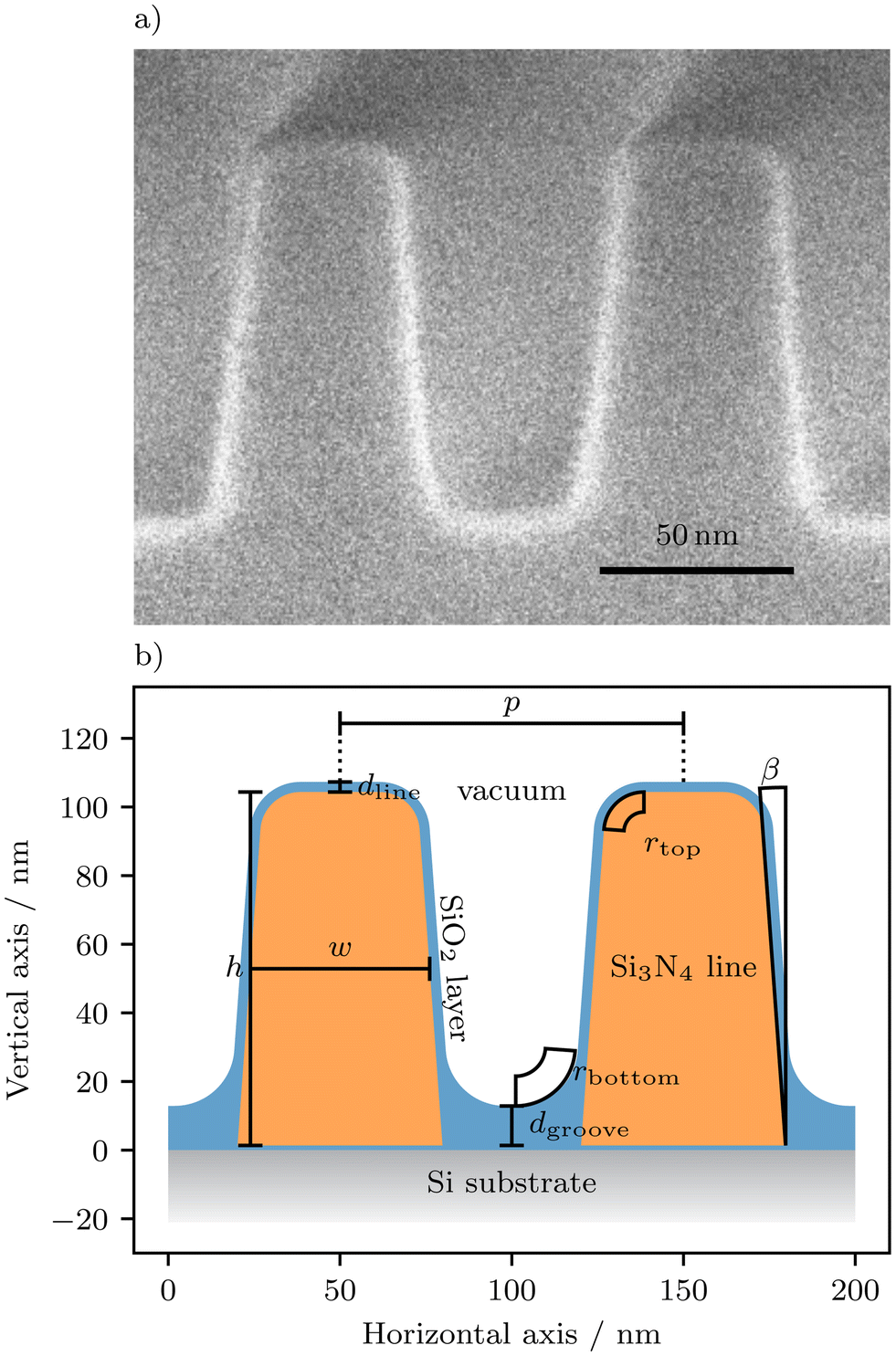 | ||
| Fig. 1 Cross-sectional view of a silicon nitride (Si3N4) nanoscale grating with a silicon dioxide (SiO2) layer on a silicon (Si) substrate made at the Helmholtz-Zentrum Berlin (HZB). A scanning electron microscopy (SEM) image of the grating profile is shown in (a), and (b) represents the parametrization scheme of its shape derived from the SEM image and the manufacturing process. The Si substrate and Si3N4 lines are separated by a native SiO2 layer with a fixed thickness of 1.35 nm. The SEM image was made by the HZB. | ||
The hybrid method combines soft X-ray scattering and fluorescence by utilizing the periodicity and composition of this nanostructure, which consists of low-Z elements of interest such as nitrogen and oxygen with L- and K-edges in the soft X-ray spectral range. This approach is effective due to the well-defined pitch (p = 100 nm) of the structure. The remaining set of varying geometry parameters is (h, w, β, rbottom, rtop, dgroove, dline). A contamination layer of carbon compounds at the sample surface is known for significant absorption of XRF radiation from inner regions of the sample. Therefore, before measuring it, the sample was cleaned at the University of Jena using a process that started with Caro's acid, followed by an ultrasonic bath in an ammonia-water solution (1![[thin space (1/6-em)]](https://www.rsc.org/images/entities/char_2009.gif) :150 NH3:H2O), water for rinsing, and spin dry. The cleaning process can cause minimal changes to the grating structure and can oxidize the surface.
:150 NH3:H2O), water for rinsing, and spin dry. The cleaning process can cause minimal changes to the grating structure and can oxidize the surface.
2.2 Theory of soft X-ray scattering on a nanoscale grating
The nanoscale grating, as described in Fig. 1, serves as a diffraction grating for soft X-rays. When monochromatized soft X-rays with wavelength λ strike the nanoscale grating with pitch p under a grazing angle of incidence αi equal to or smaller than the critical angle of total external reflection, nearly all photons are elastically scattered into distinct diffraction maxima. If the grating vector is parallel to the incidence plane (perfect conical mounting),25 the angles of the diffraction maxima can be described as follows:
 | (1) |
 | (2) |
When capturing the diffraction pattern using an area detector, it forms a semicircle over the horizon of the grating plane (Fig. 2, left). The spacial displacements between the diffraction orders are determined by the grating pitch p, the grazing angle of incidence αi and the wavelength λ. The diffraction efficiency Im(αiEi) for each order m is determined by the nanoscale grating profile's shape and the optical properties of the grating materials. The diffraction efficiency is proportional to the squared absolute value of the electric field strength far from where scattering occurs.
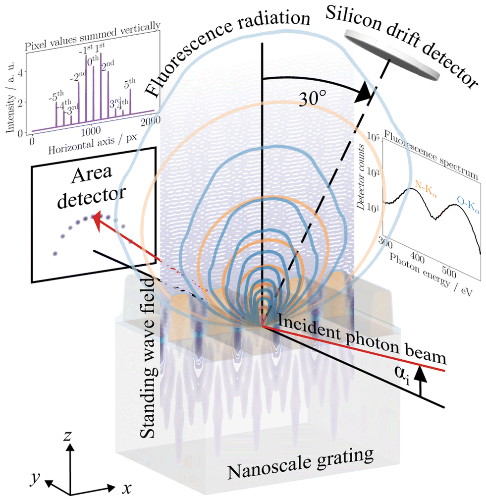 | ||
| Fig. 2 Hybrid measurement scheme in soft X-ray fluorescence scatterometry (XFS). A monochromatized photon beam illuminates a nanoscale grating with different materials at an incident angle αi, resulting in scattering or absorption and exciting various grating materials. Incoming and outgoing waves from the scattering process form the standing wave field. The scattering far-field is a diffraction pattern on the area detector in form of peaks on a semicircle. The standing wave field within the grating medium also shows how the incoming photons with appropriate energy excite the different sample materials. The photons of the stimulated emission leave the inner regions of the sample medium in different directions. The blue and orange contour lines over the sample surface visualize the intensity distribution of the simulated emission depending on the reabsorption of the leaving photons. A silicon drift detector positioned 30° off the plane of incidence captures the radiation spectrum of the stimulated emission. The spectrum includes the fluorescence emission lines of the different elements of the grating material. | ||
Fig. 2 shows the standing wave field formed by the incoming and outgoing waves at the grating, E(r,y) with r = (x,z)T. This near-field can be precisely calculated by solving Maxwell's equations using the FEM. Assuming a nanoscale grating is infinitely long and has no defects in terms of superstructure or varying pitch, a grating parametrization like that shown in Fig. 1b can be used to determine the electric field strength E(r,y) of the standing wave field. The optical properties of the materials and experimental parameters (αi and λ) are crucial for describing the interaction between grating and soft X-rays. Optical constants or the complex refractive index describe the optical properties of grating materials in relation to their interaction with soft X-rays.
Mathematically, the diffraction efficiency is proportional to the squared Fourier-transformed electric field strength of the standing wave field (Im(αi,Ei) ∝ |E(kx,m,kz,m,y)|2). This means that the efficiency depends on how strongly the wave is present in different parts of the frequency spectrum. An additional operation yields the diffraction efficiency as follows:
| Im(αi,Ei) ≈ |E(kx,m,kz,m,y)|2e−ξ2q2\!\!x,m | (3) |
2.3 Theory of soft X-ray fluorescence from a nanograting
Many characteristic fluorescence emission lines from low-Z materials lie in the soft X-ray spectral range. Therefore, GIXRF can be used for element-specific reconstruction of nanostructures.67 Depending on the incident photon energy Ei and the angular orientation of the grating with respect to the incoming photon beam, elements of different materials of the grating can be excited by the incoming photons. Different parts of the grating then emit fluorescence photons whose spectrum contains characteristic lines of atoms excited. The intensity distribution of the electric field strength of the standing wave field I(r,y) ∝ |E(r,y)|2, calculated as explained in section 2.2, determines how strong different areas of the grating cross section are stimulated. Thus, the fluorescence intensity depends on the excited area of the material Aj in the cross section of the grating. The fluorescence intensity of a certain emission line l of an element within material j can be described by the adapted and simplified Sherman equation,71 according to:
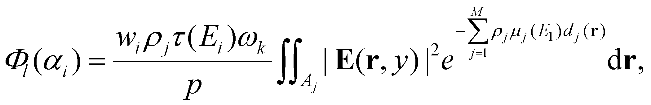 | (4) |
The mass densities of all M materials, ρj with j ∈ [1,…, M], are assumed to be constant over their areas of the grating profile Aj in an unit cell, whose width is given by the pitch p of the grating. Fundamental parameters that determine how the integral scales to the absolute fluorescence intensity are:
• The mass fraction of the fluorescent element, denoted as wi;
• The photo-ionization cross section of the relevant atomic shell for the incident photo energy Ei, denoted as τ(Ei);
• The fluorescence yield of the relevant atomic shell, ωk; and
• The mass attenuation coefficient of material j for the fluorescence energy of line l, denoted as μj(El).
The exponential term in eqn (4) describes the self-absorption of fluorescence photons of emission line l when passing all M material areas to the surface. Here, dj(r) denotes the distance to the surface of an area j, depending on the point of excitation within the grating structure r. The fluorescence intensity of emission line l calculated this way is proportional to the detected count rate for emission line l at an incident angle αi. A silicon-drift detector (SDD) measures photons arriving within the effective solid angle of detection Ω(αi)/4π and sensitivity range (Fig. 2, right).
From the raw data, the count rates Fl(αi) of each fluorescence line l are extracted through deconvolution and background subtraction.72 The emitted fluorescence intensity for emission line l is calculated as follows:
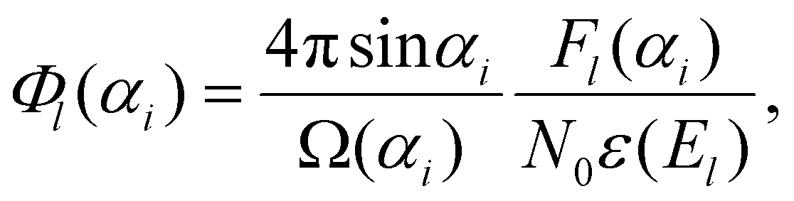 | (5) |
2.4 Instrumentation and measurement
The X-ray fluorescence scatterometry (XFS) setup used in this work allows for simultaneous soft X-ray scattering and soft X-ray fluorescence measurements. This instrument is a small and compact scattering chamber with a volume of 5 L that can be vacuumed.The scattering detection system uses a CCD, which is placed behind the sample and detects elastically scattered soft X-rays (Fig. 2, left). The setup was designed for usage with monochromatized synchrotron radiation, but it can also be used with other radiation sources like an X-ray free-electron laser (FEL) or a lab-source. Using a large collimated photon beam, different regions can be visualized on the sample surface through their different reflectance visible by imaging with the CCD. The sample stage mechanics allow for moving the sample under the photon beam. A pinhole array with pinhole sizes from 20 to 1200 μm can be used to select the part of the photon beam that illuminates the region of interest on the sample.
The setup also has an SDD, positioned on top of the chamber at an angle 30° off the plane of incidence, for detecting XRF radiation from the sample surface (Fig. 2, right). A beam shutter or filter can be brought in front of the CCD to avoid overexposure when measuring XRF radiation. When placing an appropriate filter in front of the CCD, even real-time hybrid measurements can be carried out by integrating both fluorescence spectra and diffraction images. This ensures that the hybrid measurements are taken under the same sample state.
The setup can perform scans over the grazing angle of incidence ranging from 0° to 32°. A special feature of the instrument is its ability to change the grazing angle of incidence by rotating the chamber along with its permanently mounted detectors. The captured diffraction pattern on the CCD can be used to align the sample using successive images and rotating the sample around its vertical axis with the sample stage mechanics. By moving the instrument vertically, the region of interest can be brought into the axes of both incident photon beam and SDD for measuring both scattering and fluorescence from the same sample volume. High angles of incidences and small pinhole sizes correspond to small beam footprints, allowing for probing small sample areas with elongations down to 500 μm.
The soft X-ray fluorescence scatterometer (XFS) improves upon existing setups that provide only one technique by providing a hybrid measurement approach that combines the advantages of both scattering and fluorescence analysis without the need for separate sample preparations. Thus, the XFS setup allows for more comprehensive characterization of periodic nanostructures with improved mass resolution and spatial distribution information. Unlike large GISAXS setups, the XFS setup can characterize small regions of interest with reduced beam footprint on the sample due to high angles of incidence. This allows the setup to probe specific areas within the sample volume. The permanently fixed detectors allow for stable measurement conditions.
The hybrid measurement approach utilizes the fact that some of the incoming photons are scattered at the grating structure while others get absorbed and excite atoms of the grating material if the incident photon energy has an appropriate value. The choice of the incident photon energy Ei is primarily determined by the material composition of the grating sample. Here, Ei should be significantly higher than the transition energies of the Kα-shells of nitrogen (N) and oxygen (O) at 392.4 eV and 524.9 eV, respectively,73 to excite the nitrogen and oxygen atoms and to be far from the next absorption edge. Thus, the incident photon energy is set to 680.0 eV. By scanning over the critical angle of total external reflection, a strong scattering signal is replaced by a strong fluorescence signal through increasing absorption and stimulated emission. Fig. 2 shows a sketch of the hybrid measurement scheme of soft X-ray fluorescence scatterometry (XFS) for a fixed angle of incidence. The standing wave field determines the excitation within the grating structure. The stimulated emission is influenced by the grating structure through self-absorption, depending on the exit angle of the fluorescence photons (contour lines in Fig. 2).
The fluorescence radiation emitted from the grating surface at a 30° angle off the plane of incidence is influenced differently by self-absorption through the shadowing effect than that leaving the surface in the plane of incidence. Measuring fluorescence radiation off the plane of incidence can be more sensitive to the shape of the grating compared to a conventional measurement within the plane of incidence. To increase the sensitivity of soft X-ray fluorescence, this effect is utilized in the work.
In Fig. 3, the influence of the shadowing effect on fluorescence intensity is demonstrated by comparing simulated fluorescence intensities of N-Kα and O-Kα emission lines over the grazing angle of incidence in and 30° off the plane of incidence. The comparison shows that the relative deviations for O-Kα are about ten times larger than those for N-Kα. This occurs because O-Kα fluorescence photons from grating grooves must pass through neighboring lines, while N-Kα fluorescence photons primarily leave the grating lines where they appear. Additionally, in cases with relatively high grating lines, such as this example, more fluorescence photons from inner regions of the grating lines can be detected if the pitch is sufficiently large. The figure shows that up to around 1% more N-Kα fluorescence photons can be detected from the grating line.
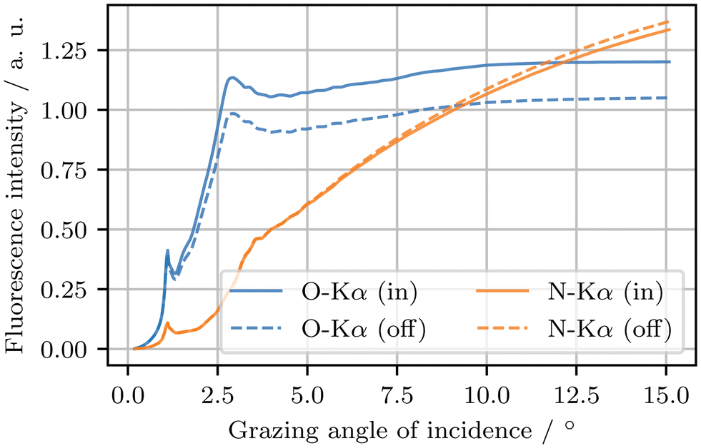 | ||
| Fig. 3 Fluorescence intensity of nitrogen (N) and oxygen (O) Kα emission lines over the grazing angle of incidence calculated with reabsorption in and 30° off the plane of incidence from a nanoscale grating model like shown in Fig. 1b in a measurement geometry shown in Fig. 2, illustrating the effect of varying angles on the emitted radiation. While off the plane of incidence more O-Kα photons get reabsorbed, a slight increase of N-Kα photons can be observed compared to the emission in the plane of incidence. | ||
Limitations on the scan over the grazing angle of incidence are given by the footprint of the photon beam on the sample surface, as well as the measurement time provided. To keep the beam footprint small, pinholes with a smaller diameter or larger incident angles can be used. The distance between an 80 μm-pinhole and the sample in the center of the chamber is set at 43 cm. As a result, the photon beam cross-section with a diameter of approximately 83 μm at the sample and the resulting beam divergence of about (0.2 × 0.2 mrad2) (width by height) are primarily determined by Fraunhofer diffraction at the pinhole.
The grazing angle of incidence affects the beam footprint on the sample. For an angular scan, the lower limit of the grazing angle (αi ≈ 2°) is set by over-illumination of the CCD due to being below the critical angle for total external reflection. At this angle, the beam footprint still covers the elongation of grating lines at about (0.08 × 2.4) mm2 (width by elongation). The upper limit of the angle of incidence is determined by the lower signal-to-noise ratio for higher-order diffraction efficiency. In this study, the scan area is reduced to scanning the grazing angle of incidence from 2° to 6° with perfect conical sample mounting.
The CCD camera captures the diffraction pattern from the grating sample, which provides the diffraction efficiency (Im(αi,Ei)) for all diffraction orders m. To achieve a high signal-to-noise ratio while maintaining linearity between integrated photon counts and actual diffraction efficiency, multiple images with short exposure times are taken for each diffraction efficiency measurement. The normalized integrated photon counts can be identified as the diffraction efficiency in arbitrary units because the area detector is not calibrated.
Fig. 4a shows the diffraction efficiency for various orders of diffraction over the grazing angle of incidence. The total uncertainty in the normalized diffraction efficiency consists of two components: the standard deviation from the combined diffraction images and a relative uncertainty of 2% due to detector inhomogeneity. Since the measured diffraction efficiency has arbitrary units, the dimensional reconstruction of the nanoscale grating uses the relative diffraction efficiency Ĩm, which is defined as the diffraction signal of higher order (m ≠ 0) divided by the diffraction signal of the zeroth order (m = 0) for each grazing angle of incidence. During fluorescence spectrum collection, a shutter in front of the CCD protects it from overexposure.
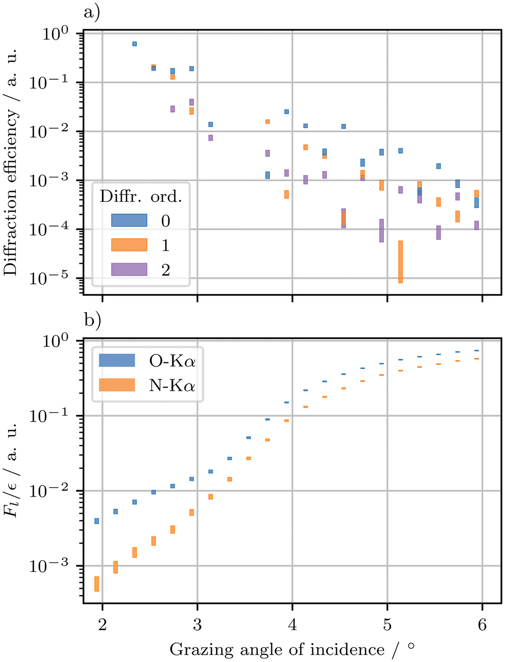 | ||
| Fig. 4 Measurement data simultaneously obtained by (a) soft X-ray scattering and (b) soft X-ray fluorescence from the silicon nitride (Si3N4) nanograting described in Fig. 1 over the grazing angle of incidence at an incident photon energy of 680.0 eV, with uncertainties shown as ±3σ for both methods. (a) shows the diffraction efficiency for some orders of diffraction and (b) shows the measured count rate of soft X-ray fluorescence of the oxygen (O) and nitrogen (N) Kα emission line. | ||
Complementing the hybrid data set over the grazing angle of incidence, Fig. 4b shows the measured count rates relative to detector efficiency El/ε(El) for the fluorescence lines of O-Kα and N-Kα. Due to the reduced photon flux behind the 80 μm-pinhole, the yield of fluorescence photons from the excited sample surface is relatively low. Consequently, the integration time of the SDD is set to 1500 seconds and the detector is brought close to less than 1 mm away from the sample surface to achieve a sufficient signal-to-noise ratio in the fluorescence spectra. This proximity between the detector and sample surface allows for detection of XRF radiation from the sample surface over a large solid angle, which explains the difference between the fluorescence curves shown in Fig. 3 and 4b.
The influence of the detector solid angle on the shape of the fluorescence intensity curve is described by the factor 4πsinαi/Ω(αi) in eqn (5). Here, the actual solid angle is unknown as the sample-detector distance cannot be accurately determined in the XFS setup. Therefore, this work uses the relative rescaled fluorescence intensity  for the dimensional reconstruction of the nanoscale grating, where the factor in eqn (5) cancels out. The relative uncertainty of the count rate for both emission lines is determined by photon fluctuations
  each.
each.
In the context of comparing scattering and fluorescence in a hybrid data set (Fig. 4), it is observed that while the diffraction efficiency decreases with increasing angle of incidence (αi) (Fig. 4a), the fluorescence intensities from oxygen and nitrogen Kα increase (Fig. 4b). This general trend can be explained by the behavior of the standing wave field within the grating structure as the grazing angle of incidence increases. As the penetration depth of the modes in the standing wave field grows, scattering efficiency decreases while absorption increases.
3 Method
To determine the sample-based parameters (h, w, β, rbottom, rtop, dgroove, dline, ξ) describing the shape of a nanoscale grating's profile shown in Fig. 1, as well as the distribution of line edge and width roughness, the inverse problem can be solved using a model of the grating (Fig. 1b) and an experiment model. The measurement data shown in Fig. 4 is used to find solutions for these parameters. Based on a set of parameters, the diffraction efficiency and fluorescence intensity can be calculated according to eqn (3) and (4) from the electric field strength of the standing wave field.This work uses the JCMsuite software (version 6.0.10) from JCMwave GmbH, Berlin74,75 to calculate the electric field strength of the standing wave field and employ a fast Fourier transform for diffraction efficiency and density integration for fluorescence intensity. In an optimization process, measured and calculated relative fluorescence intensities ( and
and  ) and diffraction efficiencies (Ĩmeasm,i and Ĩcalcm,i) are compared across various parameters to solve the inverse problem.
An optimal hybrid dimensional reconstruction of the nanoscale grating requires a balance of information from the two data sets: soft X-ray scattering and soft X-ray fluorescence. A weighting parameter, denoted as γ, is used to optimize this process by balancing a combined χ2-function (denoted as χγ2-function) that needs to be minimized. This ensures the best possible reconstruction of the nanoscale grating's dimensions using both data sets simultaneously. By adjusting the weighting parameter γ, one can control how much emphasis is placed on each measurement technique during the optimization process. For example, if γ = 1, then the reconstruction will be primarily driven by the scattering data; whereas if γ = 0, it will rely solely on fluorescence information. By finding an appropriate value for γ, one can optimize the dimensional reconstruction and show the distribution of information over different data sets in a hybrid metrology approach.
Assuming the measurement uncertainties are normal distributed and non-correlated, and soft X-ray scattering and soft X-ray fluorescence measurements are independent, the combined χ2-function can be written as:
 | (6) |
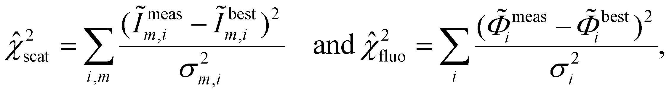 | (7) |
 represents the χ2-function value for soft X-ray scattering measurements and
  is the corresponding value for soft X-ray fluorescence for completed optimizations. This self-normalization compensates the effect of different sizes, scales, and uncertainties between the individual data sets on the weighting parameter γ. To find the right balance for the hybrid dimensional reconstruction, optimization results from a series of different parameter values γ ∈ (0,1) can be compared by their best fit χγ2-function values.
In this work, the numerical precision of the model for the standing wave field is limited to reduce computational effort. The limited precision can have a sensitive effect on the model uncertainty of the diffraction efficiency Im(αi) for some grating shapes and grazing angles of incidence. As the calculated far-field is the fast Fourier transform of the whole computational domain, this can lead to an overall model uncertainty of up to 15%. The calculated fluorescence intensity Φl,j(αi), on the other hand, results from an averaging of excitation over parts of the domain. Thus, its model uncertainty is smaller than that of the diffraction efficiency, limited by 3%.
The optical constants for Si3N4 and SiO2 are determined through a reconstruction of a layer system using soft X-ray reflectivity.67 These values are more reliable in the soft X-ray spectral range than relying solely on tabulated data, as mentioned in reference,76 where the optical constants of Si are taken from. Values for the partial photoionization cross-sections τ(680 eV) and the fluorescence yields ωk of the nitrogen Kα-shell and oxygen Kα-shell are taken from source.77
To account for small angular displacements of the grazing angle of incidence αi and the azimuthal tilt angle of the sample φ in the dimensional reconstruction, setup-based parameters (Δαi,Δφ) can determine the actual angular orientation of the grating with respect to the incoming photon beam by 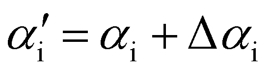 and φ′ = φ + Δφ.
This work uses differential evolution78,79 to minimize the χγ2-function, described in eqn (6), as well as  and
and  (eqn (7)) with a constant mutation rate of 80% and recombination rate of 50%. Parameter values are sampled by individual optimizations over 161 different weighting parameter values γ between 0 (fluorescence only) and 1 (scattering only) using the same parameter ranges and initial values. The solutions found can accumulate in clusters, which can be analyzed by principal component analysis (PCA)80,81 and k-means clustering,82–84 using the implementation for PCA and the KMeans class provided by the Scikit-learn library (version 1.2.2).85
4 Results and discussion
When optimizing over the weighting parameter γ, the values of the grating parameters (h, w, β, rbottom, rtop, dgroove, dline, ξ) vary over the prior ranges listed in Table 1. The variation of these values can be explained by two facts: firstly, differential evolution might not find the global minimum in a possibly multimodal solution space; and secondly, it may stop close to a minimum due to the defined termination criterion. By using principal component analysis (PCA) with 3 components and k-means clustering with a fixed number of clusters (here set at 3), three distinct clusters can be identified: Cluster Orange Circle, Cluster Blue Triangle, and Cluster Purple Square.| Parameter | Prior range | Cluster Orange Circle | Cluster Blue Triangle | Cluster Purple Square | |||||
|---|---|---|---|---|---|---|---|---|---|
| Mean | Rel. range/% | Mean | Rel. range/% | Mean | Rel. range/% | ||||
| h/nm | 87 | ⋯ | 109 | 96.2 | 16 | 97.7 | 10 | 102.2 | 4 |
| w/nm | 36 | ⋯ | 58 | 48.3 | 16 | 46.0 | 19 | 52.3 | 4 |
| β/° | 0 | ⋯ | 8.5 | 2.5 | 179 | 5.6 | 79 | 4.4 | 59 |
| rbottom/nm | 1 | ⋯ | 21 | 3.5 | 336 | 17.4 | 107 | 17.5 | 19 |
| rtop/nm | 1 | ⋯ | 15 | 10.4 | 59 | 7.3 | 76 | 11.3 | 32 |
| dgroove/nm | 1.32 | ⋯ | 14.82 | 9.1 | 62 | 6.3 | 115 | 11.2 | 30 |
| dline/nm | 1.34 | ⋯ | 4.84 | 3.6 | 21 | 2.8 | 53 | 3.0 | 21 |
| ξ/nm | 0 | ⋯ | 5 | 0.3 | 492 | 0.5 | 339 | 2.1 | 139 |
| Cluster range mean → | 148 | 100 | 38 | ||||||
Fig. 5 displays the best fit solutions for the most significant grating parameters, which are labeled with different makers (circle, triangle, square) and colors (orange, blue, purple) based on their respective clusters. These clusters represent distinct areas where multimodal best fit solutions can be found. Cluster Orange Circle and Cluster Blue Triangle exhibit larger spreads compared to that of Cluster Purple Square. Among these two clusters, Cluster Orange Circle has the largest spread. By comparing characteristics such as the spread of best fit solutions, one can determine how sensitive parameter values within a cluster are depending on the weighting in the χγ2-function. A relatively weak dependency of parameter values in a cluster suggests that the actual solution for the geometry of the nanoscale grating lies within this cluster.
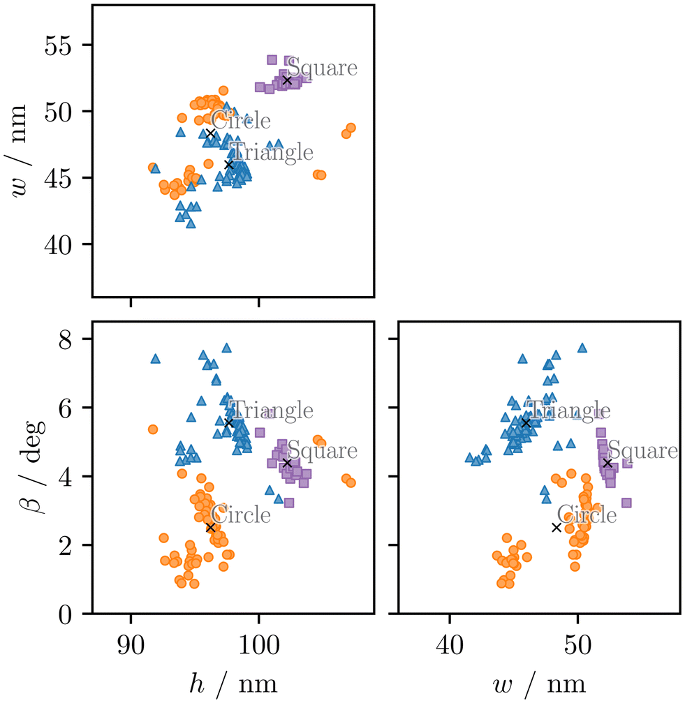 | ||
| Fig. 5 Dimensional reconstruction solutions of the Si3N4 nanograting from Fig. 1, obtained by minimizing the weighted χγ2-function in eqn (6) for various weighting parameters between γ = 0 (fluorescence only) and γ = 1 (scattering only). The solutions are grouped into clusters labeled with different markers and colors. | ||
In Fig. 6, the ranges of parameter values are normalized to their mean values for each cluster. The mean values and relative parameter ranges are listed in Table 1 along with the prior ranges used in optimization. To compare the clusters based on how much they depend on the weighting in the χγ2-function, one can calculate the average of all parameters’ relative ranges. This analysis supports the observed spread of the clusters from Fig. 5. Cluster Purple Square has the smallest relative ranges, indicating that solutions with a line height of about h = 102.2 nm are least influenced by the weighting in the χγ2-function. Comparing these results suggests that the actual solution for the grating geometry falls within the parameter ranges of Cluster Purple Square.
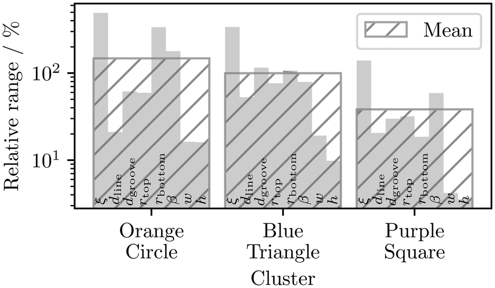 | ||
| Fig. 6 Comparison of the relative ranges for Si3N4 nanograting parameters from Table 1, plotted across different solution clusters as shown in Fig. 5. The comparison shows that Cluster Purple Square has the smallest relative parameter ranges, while Cluster Orange Circle has the largest. | ||
To further analyze the clusters, cluster labels can be assigned to the χ2-function values of the combined regression. Fig. 7a shows the sum of the normalized χ2-function values of soft X-ray scattering only (χscat2) and soft X-ray fluorescence only (χfluo2) for the best-fit solutions sampled over the weighting parameter γ, marked according to the solution clusters. The cluster labels are assigned based on the following expression:
 | (8) |
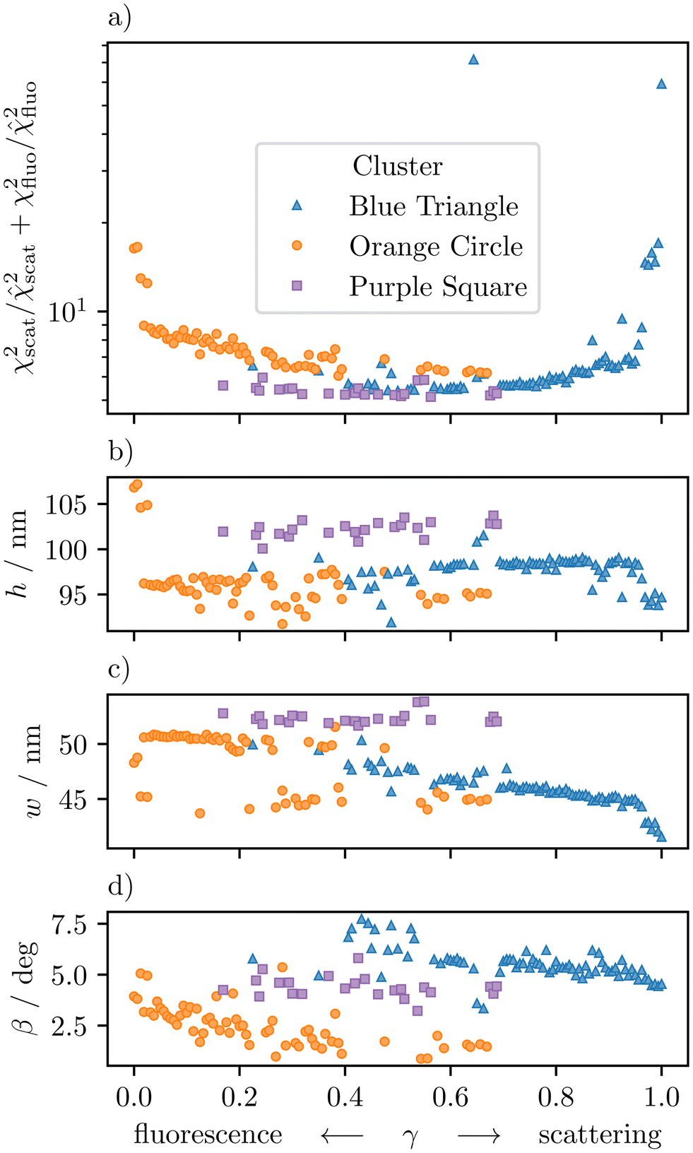 | ||
| Fig. 7 Dimensional reconstruction solutions of the Si3N4 nanograting from Fig. 1 with (a) normalized best fit solution values of the individual χ2-functions of soft X-ray scattering (χscat2) and soft X-ray fluorescence (χfluo2) and (b) the corresponding line height h, (c) the line width w, and (d) the sidewall angle β over the weighting parameter γ used in eqn (6) for optimization. All values are assigned via markers (circle, triangle, square) and colors (orange, blue, purple) to the corresponding solution clusters shown in Fig. 5. The minimum of the normalized best fit solution values indicates the best balance between information from both measurement techniques for accurate reconstruction of the grating structure. Here, the minimum is part of Cluster Purple Square whose solutions also show the smallest variance over γ. | ||
Solutions in Cluster Orange Circle and Cluster Blue Triangle can be interpreted as solutions found under the dominance of one of the two data sets in the optimization. Around the central value of the weighting parameter (γ = 0.5), solutions are influenced by both parts of the hybrid data set, which results in better compromises for fitting the hybrid data set and the appearance of solutions that belong to Cluster Purple Square. This confirms that soft X-ray scattering and soft X-ray fluorescence data are complementary.
The solutions of Cluster Purple Square seem excellent compared to those of Cluster Orange Circle and Cluster Blue Triangle because they find the best compromise in fitting the hybrid data set, while also displaying an independence from the weighting of the fit. Fig. 7b–d show the direct dependency of the solutions represented by line height h, line width w, and sidewall angle β from the weighting parameter γ. While the parameter values from Cluster Orange Circle and Cluster Blue Triangle drift and jump strongly over γ, those values from Cluster Purple Square only fluctuate around the mean value.
An appropriate weighting value for the combined regression can be found in the central region, around γ ≈ 0.16 to 0.67, where the likelihood of finding the actual solution, assigned to Cluster Purple Square, is relatively high. The fact that this central region is shifted away from the center (γ = 0.5) towards smaller γ-values can be explained by the sensitivity of soft X-ray scattering measurements to the angular position. In this case, the sensitivity is higher than that of soft X-ray fluorescence.
To compensate for the different sensitivities of measurements or the relative information content of data sets, it is important to adjust the value of the weighting parameter. This ensures that the influence of one data set with less relative information content than another data set is higher. If this balance is not achieved, the data set with a higher relative information content would dominate the optimization process, potentially leading to multimodality as a solution.
For a comparison of the results, Fig. 8 shows optimization results based on a fit of fluorescence data only (γ = 0) in the first column (Fig. 8a and b), a fit of hybrid data set using γhybrid = 0.5625, assigned to Cluster Purple Square (Fig. 8c and d), and a fit of scattering data only (γ = 1) in the third column (Fig. 8e and f). Here, the optimization results based on soft X-ray scattering and soft X-ray fluorescence data have a solution that fits only to the scattering and the fluorescence data set, respectively. The result based on the hybrid data set fits both scattering and fluorescence data; however, it does not fit as well as to individual data sets. Possible reasons for this could be an insufficient best fit or physical model like the influence of the roughness of the grating lines to soft X-ray fluorescence which is not taken into account here.
 | ||
Fig. 8 Optimization results for soft X-ray scattering and fluorescence with different values of the weighting parameter γ from eqn (6), separated by columns (γ = 0 fluorescence only, γ = 0.5625 hybrid and γ = 1 scattering only). The first three rows, (a), (c) and (e) contain the results for soft X-ray scattering over the grazing angle of incidence at incident photon energy Ei = 680 eV, represented by the relative diffraction efficiency Ĩm,i(αi,Ei) from 1st row for 1st over 0th diffraction order to 3rd row for 3rd over 0th diffraction order. The relative diffraction efficiency is rescaled by the decadic logarithm. In the last row, (b), (d) and (f) contain the results for soft X-ray fluorescence, represented by the relative fluorescence intensity  from nitrogen (N) Kα over oxygen (O) Kα over the grazing angle of incidence at incident photon energy Ei = 680 eV. The results are shown with uncertainties as ±2σ. from nitrogen (N) Kα over oxygen (O) Kα over the grazing angle of incidence at incident photon energy Ei = 680 eV. The results are shown with uncertainties as ±2σ. | ||
Other hybrid metrology approaches compare and discuss results from different techniques,53,62 make use of combined χ2-functions for combined regression,52,57,59,60 or use the results of one characterization technique as Bayesian input for another.55,56 The hybrid metrology approach in this work uses both combined regression and takes into account the relative complexity or information content of data sets from different techniques. One possible reason for different results from different characterization techniques applied on the same sample might be that the relative information content in the data sets differ from each other.
The relative information content may depend on the number of data points and the sensitivity of the technique in certain measurement sections. Weighting the combined χ2-function with a parameter, while excluding the effect of the sizes of data sets and the measurement uncertainties to the dimensional reconstruction, can optimize the dimensional reconstruction and show the distribution of information over different data sets for hybrid metrology.
5 Conclusions
This work uses a setup for soft X-ray fluorescence scatterometry, combining soft X-ray scattering and soft X-ray fluorescence in a hybrid approach to characterize a nanoscale grating made of different low-Z materials with increased unambiguity of the results. The dimensional reconstruction of the nanoscale grating is based on complementary data sets and uses combined regression. To compensate for differences in the sensitivity of the measurements or to equalize the relative information content of the data sets, the combined χ2-function used in the optimization is weighted via a parameter. This work demonstrates that the weighting parameter has a significant impact on the determined line profile of the grating. It confirms that soft X-ray scattering and soft X-ray fluorescence are complementary techniques. The study also reveals that only specific solutions based on the combined data set appear to be largely independent of the weighting parameter. The value of this parameter can provide an indication of the relative information content of the complementary data sets in relation to the model being used. This work highlights the significance of a weighting parameter for combined regression when the information content of complementary data sets is unknown. It demonstrates its applicability in determining the actual solution of grating line profiles over ambiguous solutions.Author contributions
L. M. Lohr: conceptualization, methodology, data curation, formal analysis, investigation, validation, writing–original draft, writing–review & editing, visualization. R. Ciesielski: conceptualization, data curation, formal analysis, investigation, writing–review & editing, mentorship. V.-B. Truong: data curation, writing–review & editing. V. Soltwisch: conceptualization, methodology, validation, resources, supervision, project administration, funding acquisition, writing–review & editing.Data availability
Data for this article, including measurement data, optimization results and fit data are available at Zenodo at https://doi.org/10.5281/zenodo.14026160.Conflicts of interest
There are no conflicts to declare.Acknowledgements
The project (grant agreement number 101096772) is supported by Chips Joint Undertaking and its members, including the top-up funding of Belgium and the Netherlands.The authors would like to thank Thomas Siefke and his colleagues at the University of Jena for cleaning the Si3N4 grating sample. They also express gratitude towards Philipp Hönicke from the Helmholtz-Zentrum Berlin (HZB) for engaging in fruitful discussions.
References
- IEEE IRDS, International Roadmap for Devices and Systems 2023 Update: Metrology, IEEE technical report, IEEE, 2023.
- N. G. Orji, M. Badaroglu, B. M. Barnes, C. Beitia, B. D. Bunday, U. Celano, R. J. Kline, M. Neisser, Y. Obeng and A. E. Vladar, Nat. Electron., 2018, 1, 532–547 CrossRef PubMed.
- D. C. Joy, AIP Conf. Proc., 2003, 683, 619–626 CrossRef.
- M. Knoll and E. Ruska, Z. Phys., 1932, 78, 318–339 CrossRef CAS.
- T. T. Sheng and R. B. Marcus, J. Electrochem. Soc., 1980, 127, 737 CrossRef CAS.
- M. von Ardenne, Z. Phys., 1938, 109, 553–572 CrossRef.
- A. V. Crewe, M. Isaacson and D. Johnson, Rev. Sci. Instrum., 1969, 40, 241–246 CrossRef.
- H. P. Kleinknecht and H. Meier, J. Electrochem. Soc., 1978, 125, 798 CrossRef CAS.
- S. S. H. Naqvi, S. Gaspar, K. Hickman, K. Bishop and J. R. McNeil, Appl. Opt., 1992, 31, 1377–1384 CrossRef CAS PubMed.
- J. R. McNeil, S. S. H. Naqvi, S. M. Gaspar, K. C. Hickman, K. P. Bishop, L. M. Milner, R. H. Krukar and G. A. Petersen, Solid State Technol., 1993, 36, 29–32 Search PubMed.
- C. J. Raymond, M. R. Murnane, S. Sohail, H. Naqvi and J. R. McNeil, J. Vac. Sci. Technol., B:Nanotechnol. Microelectron.:Mater., Process., Meas., Phenom., 1995, 13, 1484–1495 CAS.
- D. L. Ho, C. Wang, E. K. Lin, R. L. Jones and W. Wu, AIP Conf. Proc., 2007, 931, 382–386 CrossRef CAS.
- G. Binnig, C. F. Quate and C. Gerber, Phys. Rev. Lett., 1986, 56, 930–933 CrossRef PubMed.
- R. G. Dixson, A. Guerry, M. H. Bennett, T. V. Vorburger and B. D. Bunday, Metrology, Inspection, and Process Control for Microlithography XVII, 2003, 5038, 150–165 Search PubMed.
- R. Fitzgerald, K. Keil and K. F. J. Heinrich, Science, 1968, 159, 528–530 CrossRef CAS PubMed.
- E. Gatti and P. Rehak, Nucl. Instrum. Methods Phys. Res., 1984, 225, 608–614 CrossRef CAS.
- R. Tsuneta, M. Koguchi, K. Nakamura and A. Nishida, J. Electron Microsc., 2002, 51, 167–171 CrossRef CAS PubMed.
- A. Emami-Naeini and D. de Roover, Proc. Symposium To Honor Bill Wolovich, 47th IEEE Conference on Decision and Control, Cancun, Mexico, 2008.
- M. Guillaume, N. Noailly, M. Pichot and J. Buevoz, Microelectron. Eng., 1985, 3, 211–218 CrossRef.
- R. A. Allen, H. J. Patrick, M. Bishop, T. A. Germer, R. Dixson, W. F. Guthrie and M. W. Cresswell, 2007 IEEE International Conference on Microelectronic Test Structures, 2007, pp. 20–25.
- M. Wurm, J. Endres, J. Probst, M. Schoengen, A. Diener and B. Bodermann, Opt. Express, 2017, 25, 2460–2468 CrossRef CAS PubMed.
- A. Fernández Herrero, M. Pflüger, J. Puls, F. Scholze and V. Soltwisch, Opt. Express, 2021, 29, 35580–35591 CrossRef PubMed.
- L. M. Lohr, R. Ciesielski, S. Glabisch, S. Schröder, S. Brose and V. Soltwisch, Appl. Opt., 2023, 62, 117–132 CrossRef CAS PubMed.
- J. R. Levine, J. B. Cohen, Y. W. Chung and P. Georgopoulos, J. Appl. Crystallogr., 1989, 22, 528–532 CrossRef CAS.
- J. Wernecke, M. Krumrey, A. Hoell, R. J. Kline, H.-K. Liu and W.-L. Wu, J. Appl. Crystallogr., 2014, 47, 1912–1920 CrossRef CAS.
- H. Gross, M.-A. Henn, S. Heidenreich, A. Rathsfeld and M. Bär, Appl. Opt., 2012, 51, 7384–7394 CrossRef CAS PubMed.
- A. Fernández Herrero, M. Pflüger, J. Probst, F. Scholze and V. Soltwisch, Opt. Express, 2019, 27, 32490–32507 CrossRef PubMed.
- A. Fernández Herrero, F. Scholze, G. Dai and V. Soltwisch, Nanomanuf. Metrol., 2022, 5, 149–158 CrossRef.
- M.-A. Henn, Ph.D. thesis, Technischen Universität Berlin, 2013.
- B. Bodermann, B. Loechel, F. Scholze, G. Dai, J. Wernecke, J. Endres, J. Probst, M. Schoengen, M. Krumrey, P.-E. Hansen and V. Soltwisch, Optical Micro- and Nanometrology V, 2014, 9132, 56–67 Search PubMed.
- Y.-S. Ku, C.-L. Yeh, Y.-C. Chen, C.-W. Lo, W.-T. Wang and M.-C. Chen, Opt. Express, 2016, 24, 28014–28025 CrossRef CAS PubMed.
- L. Bahrenberg, S. Danylyuk, S. Glabisch, M. Ghafoori, S. Schröder, S. Brose, J. Stollenwerk and P. Loosen, Opt. Express, 2020, 28, 20489–20502 CrossRef CAS PubMed.
- C. Porter, T. Coenen, N. Geypen, S. Scholz, L. van Rijswijk, H.-K. Nienhuys, J. Ploegmakers, J. Reinink, H. Cramer, R. van Laarhoven, D. O’Dwyer, P. Smorenburg, A. Invernizzi, R. Wohrwag, H. Jonquiere, J. Reinhardt, O. El Gawhary, S. Mathijssen, P. Engblom, H. Chin, W. T. Blanton, S. Ganesan, B. Krist, F. Gstrein and M. Phillips, Metrology, Inspection, and Process Control XXXVII, 2023, 12469, 412–420 Search PubMed.
- M. G. Moharam and T. K. Gaylord, J. Opt. Soc. Am., 1981, 71, 811–818 CrossRef.
- M. G. Moharam, E. B. Grann, D. A. Pommet and T. K. Gaylord, J. Opt. Soc. Am. A, 1995, 12, 1068–1076 CrossRef.
- M. G. Moharam, D. A. Pommet, E. B. Grann and T. K. Gaylord, J. Opt. Soc. Am. A, 1995, 12, 1077–1086 CrossRef.
- P. Lalanne and G. M. Morris, J. Opt. Soc. Am. A, 1996, 13, 779–784 CrossRef.
- L. Li, J. Opt. Soc. Am. A, 1997, 14, 2758–2767 CrossRef.
- H. P. Urbach, SIAM J. Numer. Anal., 1991, 28, 697–710 CrossRef.
- G. Bao, SIAM J. Numeri. Anal., 1995, 32, 1155–1169 CrossRef.
- J. Elschner, R. Hinder and G. Schmidt, Adv. Comput. Math., 2002, 16, 139–156 CrossRef.
- V. Soltwisch, A. Fernández Herrero, M. Pflüger, A. Haase, J. Probst, C. Laubis, M. Krumrey and F. Scholze, J. Appl. Crystallogr., 2017, 50, 1524–1532 CrossRef CAS.
- F. Zenhausern, Y. Martin and H. K. Wickramasinghe, Science, 1995, 269, 1083–1085 CrossRef CAS PubMed.
- D. Siebenkotten, B. Kästner, M. Marschall, A. Hoehl and S. Amakawa, Opt. Express, 2024, 32, 23882–23893 CrossRef CAS PubMed.
- Y. Yoneda and T. Horiuchi, Rev. Sci. Instrum., 1971, 42, 1069–1070 CrossRef CAS PubMed.
- D. K. G. de Boer, Phys. Rev. B:Condens. Matter Mater. Phys., 1991, 44, 498–511 CrossRef CAS PubMed.
- F. Reinhardt, S. H. Nowak, B. Beckhoff, J.-C. Dousse and M. Schoengen, J. Anal. At. Spectrom., 2014, 29, 1778–1784 RSC.
- L. G. Parratt, Phys. Rev., 1954, 95, 359–369 CrossRef.
- D. Ingerle, M. Schiebl, C. Streli and P. Wobrauschek, Rev. Sci. Instrum., 2014, 85, 083110 CrossRef CAS PubMed.
- P. Hönicke, B. Detlefs, E. Nolot, Y. Kayser, U. Mühle, B. Pollakowski and B. Beckhoff, J. Vac. Sci. Technol., A, 2019, 37, 041502 CrossRef.
- D. Ingerle, W. Artner, K. Hradil and C. Streli, Powder Diffr., 2020, 35, S29–S33 CrossRef CAS.
- S. Melhem, Y. Ménesguen, E. Nolot and M.-C. Lépy, X-Ray Spectrom., 2023, 52, 412–422 CrossRef CAS.
- M. Yan, J. Bardeau, G. Brotons, T. Metzger and A. Gibaud, KEK Proc, 2006, pp. 107–116 Search PubMed.
- A. Vaid, B. B. Yan, Y. T. Jiang, M. Kelling, C. Hartig, J. Allgair, P. Ebersbach, M. Sendelbach, N. Rana, A. Katnani, E. Mclellan, C. Archie, C. Bozdog, H. Kim, M. Sendler, S. Ng, B. Sherman, B. Brill, I. Turovets and R. Urensky, Metrology, Inspection, and Process Control for Microlithography XXV, 2011, 7971, 21–40 Search PubMed.
- R. M. Silver, N. F. Zhang, B. M. Barnes, H. Zhou, J. Qin and R. Dixson, Metrology, Inspection, and Process Control for Microlithography XXV, 2011, 7971, 381–391 Search PubMed.
- R. M. Silver, B. M. Barnes, N. F. Zhang, H. Zhou, A. Vladár, J. Villarrubia, J. Kline, D. Sunday and A. Vaid, Metrology, Inspection, and Process Control for Microlithography XXVIII, 2014, p. 905004 Search PubMed.
- M.-A. Henn, R. M. Silver, J. S. Villarrubia, N. F. Zhang, H. Zhou, B. M. Barnes, B. Ming and A. E. Vladár, J. Micro/Nanolithogr., MEMS, MOEMS, 2015, 14(4), 044001 CrossRef PubMed.
- N. Griesbach Schuch, Theses, Université Grenoble Alpes, 2017.
- L. Siaudinyte, P.-E. Hansen, R. Koops, J. Xu and E. Peiner, Meas. Sci. Technol., 2023, 34, 094008 CrossRef CAS.
- P.-E. Hansen, S. R. Johannsen, S. A. Jensen and J. S. M. Madsen, Front. Phys., 2022, 9, 791459 CrossRef.
- J. Stöhr, in Principles, Techniques, and Instrumentation of NEXAFS, ed. J. Stöhr, Springer Berlin Heidelberg, Berlin, Heidelberg, 1992, pp. 114–161 Search PubMed.
- I. Murataj, A. Angelini, E. Cara, S. Porro, B. Beckhoff, Y. Kayser, P. Hönicke, R. Ciesielski, C. Gollwitzer, V. Soltwisch, F. Perez-Murano, M. Fernandez-Regulez, S. Carignano, L. Boarino, M. Castellino and F. Ferrarese Lupi, ACS Appl. Mater. Interfaces, 2023, 15, 57992–58002 CrossRef CAS PubMed.
- D. B. Williams, A. J. Papworth and M. Watanabe, Microscopy, 2002, 51, S113–S126 Search PubMed.
- A. A. Herzing, M. Watanabe, J. K. Edwards, M. Conte, Z.-R. Tang, G. J. Hutchings and C. J. Kiely, Faraday Discuss., 2008, 138, 337–351 RSC.
- V. Soltwisch, P. Hönicke, Y. Kayser, J. Eilbracht, J. Probst, F. Scholze and B. Beckhoff, Nanoscale, 2018, 10, 6177–6185 RSC.
- P. Hönicke, A. Andrle, Y. Kayser, K. V. Nikolaev, J. Probst, F. Scholze, V. Soltwisch, T. Weimann and B. Beckhoff, Nanotechnology, 2020, 31, 505709 CrossRef PubMed.
- A. Andrle, P. Hönicke, G. Gwalt, P.-I. Schneider, Y. Kayser, F. Siewert and V. Soltwisch, Nanomaterials, 2021, 11, 2079–4991 CrossRef PubMed.
- A. Andrle, Ph.D. thesis, Technische Universität Berlin, Inst. Optik und Atomare Physik, 2023.
- R. Ciesielski, L. M. Lohr, A. Fernández Herrero, A. Fischer, A. Grothe, H. Mentzel, F. Scholze and V. Soltwisch, Rev. Sci. Instrum., 2023, 94, 013904 CrossRef CAS PubMed.
- M. H. Pflüger, Ph.D. thesis, Humboldt Universitaet zu Berlin, Germany, 2020.
- J. Sherman, Spectrochim. Acta, 1955, 7, 283–306 CrossRef CAS.
- F. Scholze, B. Beckhoff, M. Kolbe, M. Krumrey, M. Müller and G. Ulm, Microchim. Acta, 2006, 155, 275–278 CrossRef CAS.
- G. H. Zschornack, in Handbook of X-ray Data, Springer Science & Business Media, 2007, ch. 5, pp. 184–185 Search PubMed.
- JCMsuite [Commercial computer software], https://jcmwave.com/.
- S. Burger, J. Pomplun and F. Schmidt, in Finite Element Methods for Computational Nano-optics, ed. B. Bhushan, Springer Netherlands, Dordrecht, 2012, pp. 837–843 Search PubMed.
- B. Henke, E. Gullikson and J. Davis, At. Data Nucl. Data Tables, 1993, 54, 181–342 CrossRef CAS.
- W. Elam, B. Ravel and J. Sieber, Radiat. Phys. Chem., 2002, 63, 121–128 CrossRef CAS.
- R. Storn and K. Price, J. Glob. Optim., 1997, 11, 341–359 CrossRef.
- P. Virtanen, R. Gommers, T. E. Oliphant, M. Haberland, T. Reddy, D. Cournapeau, E. Burovski, P. Peterson, W. Weckesser, J. Bright, S. J. van der Walt, M. Brett, J. Wilson, K. J. Millman, N. Mayorov, A. R. J. Nelson, E. Jones, R. Kern, E. Larson, C. J. Carey, İ. Polat, Y. Feng, E. W. Moore, J. VanderPlas, D. Laxalde, J. Perktold, R. Cimrman, I. Henriksen, E. A. Quintero, C. R. Harris, A. M. Archibald, A. H. Ribeiro, F. Pedregosa, P. van Mulbregt and SciPy 1.0 Contributors, Nat. Methods, 2020, 17, 261–272 CrossRef CAS PubMed.
- K. Pearson, The London, Edinburgh, and Dublin Philosophical Magazine and Journal of Science, 1901, vol. 2, pp. 559–572 Search PubMed.
- H. Hotelling, J. Educ. Psychol., 1933, 24, 417–441 Search PubMed.
- J. MacQueen, Proceedings of 5-th Berkeley Symposium on Mathematical Statistics and Probability, 1967, pp. 281–297.
- S. P. Lloyd, IEEE Trans. Inf. Theory, 1982, 28, 129–137 CrossRef.
- E. W. Forgy, Biometrics, 1965, 21, 768–769 Search PubMed.
- F. Pedregosa, G. Varoquaux, A. Gramfort, V. Michel, B. Thirion, O. Grisel, M. Blondel, P. Prettenhofer, R. Weiss and V. Dubourg, et al., J. Mach. Learn. Res., 2011, 12, 2825–2830 Search PubMed.
| This journal is © The Royal Society of Chemistry 2025 |